Download as PDF, PPTX


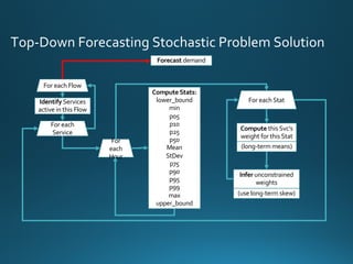
![[𝜇 − 𝑍 ∗ 𝜎, 𝜇 + 𝑍 ∗ 𝜎]
• The 𝑍 is arbitrary
• Assumptions about the distribution:
• Mean andVariance defined
• Gaussian (Symmetrical)
• Stationary
• No outliers
• Simple math:
• Addition
• Regression
• TSA Forecasting](https://image.slidesharecdn.com/performanceorcapacitycmg16-161109151847/85/Performance-OR-Capacity-CMGimPACt2016-9-320.jpg)
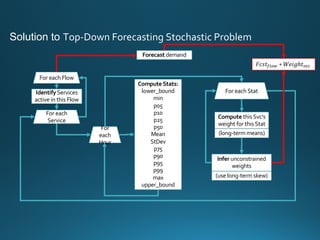
![[𝜇 − 𝑍 ∗ 𝜎, 𝜇 + 𝑍 ∗ 𝜎] [𝜇 − 𝑍 𝟏 ∗ 𝜎, 𝜇 + 𝑍 𝟐 ∗ 𝜎]
𝑆𝑎𝑚𝑝𝑙𝑖𝑛𝑔:
With enough random samples, their
means will be Gaussian
(Central LimitTheorem)
𝐷𝑎𝑡𝑎 𝑇𝑟𝑎𝑛𝑠𝑓𝑜𝑟𝑚𝑎𝑡𝑖𝑜𝑛:
• log
• exp
• Box-CoxFor Capacity Planning: For Monitoring:](https://image.slidesharecdn.com/performanceorcapacitycmg16-161109151847/85/Performance-OR-Capacity-CMGimPACt2016-10-320.jpg)
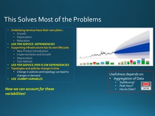
![User Metrics:
• throughput
• latency
• data loss
• data loss & latency
• latency & data loss
TheWhirlpool of Metrics
For Monitoring
Real metrics:
• # of Packets in Flight
• # of Packets in Queue or Lost
For Capacity Planning
Traditional Metrics in Planning:
• 𝑇ℎ𝑟𝑜𝑢𝑔ℎ𝑝𝑢𝑡 [Gbps]
• 𝐿𝑎𝑡𝑒𝑛𝑐𝑦hijklm
• 𝐿𝑎𝑡𝑒𝑛𝑐𝑦hinl = 𝑙𝑜𝑎𝑑𝑖𝑛𝑔 || 𝑟𝑒𝑎𝑠𝑠𝑒𝑚𝑏𝑙𝑦
• Packets get queued and blocked.
• Bits may be bursty while packets are smooth.
• Reverse statement is true as well.
• 𝐿𝑎𝑡𝑒𝑛𝑐𝑦hijklm = 𝑡𝑟𝑎𝑛𝑠𝑝𝑜𝑟𝑡 + 𝑞𝑢𝑒𝑢𝑒𝑖𝑛𝑔
• Packets need capacity.
• Packet sizes vary => capacity [Gbps]
Example:
320 𝐺𝑏𝑝𝑠 = 26.7𝑀 ∗
1.5𝑘𝐵 ∗ 8 𝑏𝑖𝑡𝑠
𝑠𝑒𝑐
320 𝐺𝑏𝑝𝑠 = 10 ∗
4𝐺𝑖𝐵 ∗ 8 𝑏𝑖𝑡𝑠
𝑠𝑒𝑐
Traditional Metrics for Monitoring:
• % Utilization
• Packet Loss Rate](https://image.slidesharecdn.com/performanceorcapacitycmg16-161109151847/85/Performance-OR-Capacity-CMGimPACt2016-18-320.jpg)
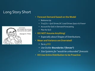
![Time, Rate, Count, and Utilization
𝑃 𝑞 = 𝐸𝑟𝑙𝑎𝑛𝑔𝐶 (𝑁, 𝐶)
Packet Queueing:
𝑃 𝑏 = 𝐸𝑟𝑙𝑎𝑛𝑔𝐵 (𝑁, 𝐶)
Packet Blocking:
2012 paper
𝑁 = 𝑃𝑃𝑆 ∗ 𝐿𝑎𝑡𝑒𝑛𝑐𝑦
𝐿𝑎𝑡𝑒𝑛𝑐𝑦 =
1
2
∗ 𝑅𝑇𝑇 + 𝑇€•‚‚
𝑏𝑝𝑠 = 𝑃𝑃𝑆 ∗
𝑏𝑖𝑡𝑠
𝑝𝑎𝑐𝑘𝑒𝑡
𝐶 = 𝑚𝑎 𝑥 𝑃𝑃𝑆 ∗
1
2
∗ 𝑅𝑇𝑇
2006 paper
(CPU centric)
• Utilization CAN BE useless
• If the metric does not
reflect what it is used for.
links were utilized
near 100% [
€hƒ
€hƒ
] but
no packet drops](https://image.slidesharecdn.com/performanceorcapacitycmg16-161109151847/85/Performance-OR-Capacity-CMGimPACt2016-19-320.jpg)
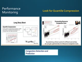
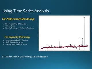
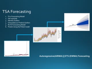
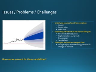
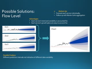
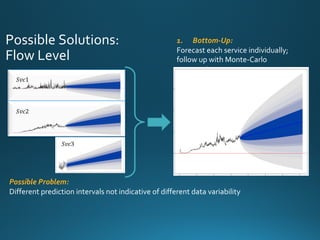
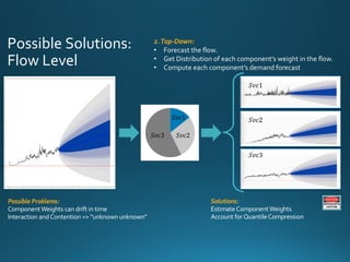


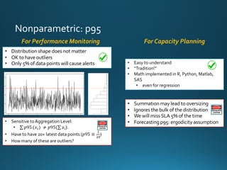
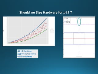
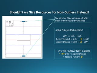
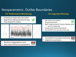
The document discusses various approaches and metrics for performance analysis and capacity planning in IT, highlighting the importance of understanding distinctions between performance and capacity metrics. It details methodologies for analyzing data trends, identifying outliers, and making forecasts to optimize resource allocation while addressing common challenges such as variability and changing demands. Additionally, it emphasizes the necessity of avoiding standardized metrics, advocating instead for tailored, data-driven strategies that account for the entirety of data distributions.