Capacity Management and Planning_ Data Science, Queueing, Optimization and other good things.pdf
1.
Capacity Management andPlanning:
Data Science, Queueing, Optimization
and other good things
Alex Gilgur, PhD
Principal Data Scientist
2.
Abstract
Capacity Management (CapMan)and Planning (CapPlan) are two sides of the same coin –
ensuring that we can deliver the best experience to the customer at the lowest cost to us.
It is traditionally the most operations-research (OR) - heavy side of any technical
infrastructure.
This talk dives into capacity management and planning, why we do it, and how we do it.
2
3.
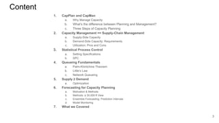
Content
1. CapPlan andCapMan
a. Why Manage Capacity
b. What’s the difference between Planning and Management?
c. Three Steps of Capacity Planning
2. Capacity Management == Supply-Chain Management
a. Supply-Side Capacity
b. Demand-Side Capacity: Requirements
c. Utilization: Pros and Cons
3. Statistical Process Control
a. Setting Specifications
b. SPC
4. Queueing Fundamentals
a. Palm-Khintchine Theorem
b. Little’s Law
c. Network Queueing
5. Supply ≥ Demand
a. Optimization
6. Forecasting for Capacity Planning
a. Motivation & Methods
b. Methods: a 30,000-ft View
c. Ensemble Forecasting: Prediction Intervals
d. Model Monitoring
7. What we Covered
3
4.
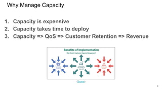
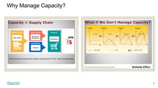
Why Manage Capacity
1.Capacity is expensive
2. Capacity takes time to deploy
3. Capacity => QoS => Customer Retention => Revenue
(Source)
4
5.
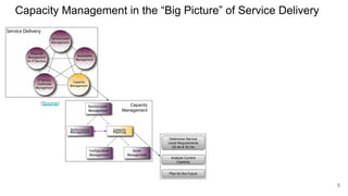
Capacity Management inthe “Big Picture” of Service Delivery
Capacity
Management
Determine Service
Level Requirements
(SLAs & SLOs)
Analyze Current
Capacity
Plan for the Future
(Source)
5
6.
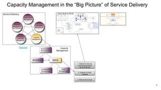
Capacity Management inthe “Big Picture” of Service Delivery
Capacity
Management
1. Determine Service
Level Requirements
(SLAs & SLOs)
2. Analyze Current
Capacity
3. Plan for the Future
(Source)
From SLAs to SLOs
6
7.
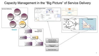
Capacity Management inthe “Big Picture” of Service Delivery
Capacity
Management
Determine Service
Level Requirements
(SLAs & SLOs)
Analyze Current
Capacity
Plan for the Future
(Source)
From SLAs to SLOs
Simulation Optimization
7
8.
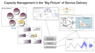
Capacity Management inthe “Big Picture” of Service Delivery
Capacity
Management
Determine Service
Level Requirements
(SLAs & SLOs)
Analyze Current
Capacity
Plan for the Future
(Source)
From SLAs to SLOs
Simulation Optimization
Forecasting
8
Supply-Chain Management andCapacity Management
Performance
Monitoring
Planning
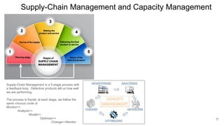
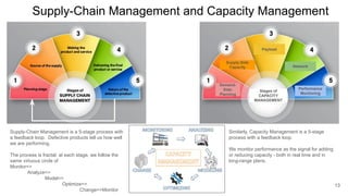
Supply-Chain Management is a 5-stage process with
a feedback loop. Defective products tell us how well
we are performing.
The process is fractal: at each stage, we follow the
same virtuous circle of
Monitor=>
Analyze=>
Model=>
Optimize=>
Change=>Monitor
11
12.
Supply-Chain Management andCapacity Management
Performance
Monitoring
Planning
Payload
Network
Performance
Monitoring
Supply-Chain Management is a 5-stage process with
a feedback loop. Defective products tell us how well
we are performing.
The process is fractal: at each stage, we follow the
same virtuous circle of
Monitor=>
Analyze=>
Model=>
Optimize=>
Change=>Monitor
Supply-Side
Capacity
Demand-
Side:
Planning
12
Stages of
CAPACITY
MANAGEMENT
13.
Supply-Chain Management andCapacity Management
Performance
Monitoring
Planning
Payload
Network
Performance
Monitoring
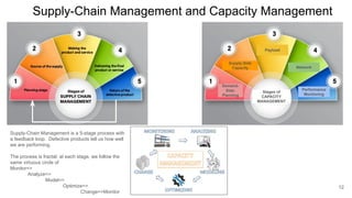
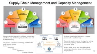
Supply-Chain Management is a 5-stage process with
a feedback loop. Defective products tell us how well
we are performing.
The process is fractal: at each stage, we follow the
same virtuous circle of
Monitor=>
Analyze=>
Model=>
Optimize=>
Change=>Monitor
Similarly, Capacity Management is a 5-stage
process with a feedback loop.
We monitor performance as the signal for adding
or reducing capacity - both in real time and in
long-range plans.
Supply-Side
Capacity
Demand-
Side:
Planning
13
Stages of
CAPACITY
MANAGEMENT
14.
Supply-Chain Management andCapacity Management
Performance
Monitoring
Planning
Similarly, Capacity Management is a 5-stage
process with a feedback loop.
We monitor performance as the signal for adding
or reducing capacity - both in real time and in
long-range plans.
At each stage, we do fault and performance
monitoring and control, along with root-cause
analysis (RCA)
Supply-Side
Capacity
Payload
Network
Performance
Monitoring
Demand-
Side:
Planning
Supply-Chain Management is a 5-stage process with
a feedback loop. Defective products tell us how well
we are performing.
The process is fractal: at each stage, we follow the
same virtuous circle of
Monitor=>
Analyze=>
Model=>
Optimize=>
Change=>Monitor
14
Stages of
CAPACITY
MANAGEMENT
15.
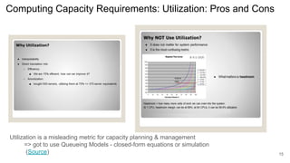
Computing Capacity Requirements:Utilization: Pros and Cons
15
Utilization is a misleading metric for capacity planning & management
=> got to use Queueing Models - closed-form equations or simulation
(Source)
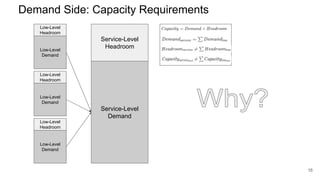
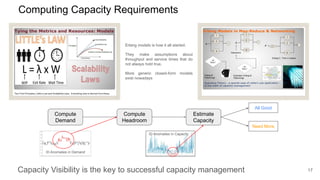
Computing Capacity Requirements
17
Compute
Demand
Compute
Headroom
Estimate
Capacity
AllGood
Need More
ID Anomalies in Demand
ID Anomalies in Capacity
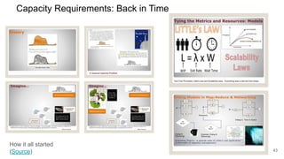
Erlang models is how it all started.
They make assumptions about
throughput and service times that do
not always hold true.
More generic closed-form models
exist nowadays
Capacity Visibility is the key to successful capacity management
18.
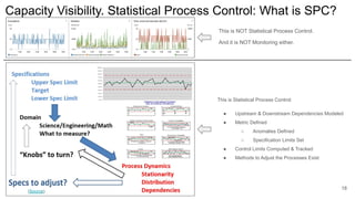
Capacity Visibility. StatisticalProcess Control: What is SPC?
18
This is NOT Statistical Process Control.
And it is NOT Monitoring either.
This is Statistical Process Control:
● Upstream & Downstream Dependencies Modeled
● Metric Defined
○ Anomalies Defined
○ Specification Limits Set
● Control Limits Computed & Tracked
● Methods to Adjust the Processes Exist
(Source)
19.
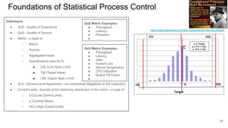
Foundations of StatisticalProcess Control
19
Definitions
● QoE - Quality of Experience
● QoS - Quality of Service
● Metric - a tuple of:
○ Name,
○ Source,
○ Aggregation level
○ Specifications (aka SLO)
■ LSL (Low Spec Limit)
■ Tgt (Target Value)
■ USL (Upper Spec Limit)
● SLA - Service Level Agreement - our contractual obligations to the customers
● Control Limits - bounds of the stationary distribution of the metric - a tuple of
○ LCL(Low Control Limit),
○ μ (Central Value),
○ HCL (High Control Limit)
QoE Metric Examples:
● Throughput
● Latency
● Pixelation
● ... ... ...
QoS Metric Examples:
● Throughput
● Latency
● Jitter
● Packet Loss
● Device Temperature
● CPU Utilization
● Queue Fill Factor
● ... ... ...
https://edmondbusiness.com/2021/02/gentlemen-this-is-a-football/
20.
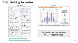
SPC: Defining Anomalies
20
Rules-BasedStatistical
https://en.wikipedia.org/wiki/Nelson_rules
https://en.wikipedia.org/wiki/Western_Electric_rules
How Significant are these Anomalies?
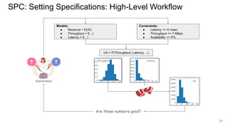
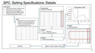
We need SPECIFICATIONS
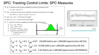
SPC: Tracking ControlLimits: SPC Measures
24
Z
st
= 2: Z
lt
= 0.5: C
pk
= 0.67: 310,000 defects per 1,000,000 opportunities (68.2%);
Z
st
= 3: Z
lt
= 1.5: C
pk
= 1.0: 67,000 defects per 1,000,000 opportunities (93.3%)
Z
st
= 6: Z
lt
= 4.5: C
pk
= 2.0: 3.45 defects per 1,000,000 opportunities (99.999965%)
Source:
https://www.six-sigma-material.com/Tables.html
25.
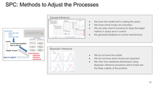
SPC: Methods toAdjust the Processes
25
Causal Inference
● We have the model built in setting the specs
● We know which knobs are important
● We can play what-if scenarios to keep the target
metrics in specs and in control
● We generate feedback to control mechanisms
Bayesian Inference
● We do not have the model
● We do not know which knobs are important
● We infer from statistical distributions using
Bayesian inference procedure which knobs are
the likely culprits of the problem
26.
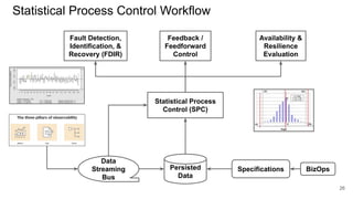
Statistical Process ControlWorkflow
26
Statistical Process
Control (SPC)
Fault Detection,
Identification, &
Recovery (FDIR)
Feedback /
Feedforward
Control
Availability &
Resilience
Evaluation
Persisted
Data
Data
Streaming
Bus
BizOps
Specifications
27.
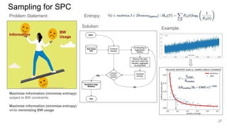
Sampling for SPC
27
Information
BW
Usage
ProblemStatement: Entropy:
Maximize information (minimize entropy)
subject to BW constraints
Maximize information (minimize entropy)
while minimizing BW usage
Solution: Example:
28.
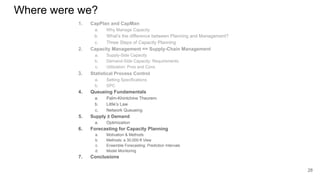
Where were we?
1.CapPlan and CapMan
a. Why Manage Capacity
b. What’s the difference between Planning and Management?
c. Three Steps of Capacity Planning
2. Capacity Management == Supply-Chain Management
a. Supply-Side Capacity
b. Demand-Side Capacity: Requirements
c. Utilization: Pros and Cons
3. Statistical Process Control
a. Setting Specifications
b. SPC
4. Queueing Fundamentals
a. Palm-Khintchine Theorem
b. Little’s Law
c. Network Queueing
5. Supply ≥ Demand
a. Optimization
6. Forecasting for Capacity Planning
a. Motivation & Methods
b. Methods: a 30,000-ft View
c. Ensemble Forecasting: Prediction Intervals
d. Model Monitoring
7. Conclusions
28
29.
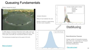
Queueing Fundamentals
What’s happeninghere?
In 2008, Nagoya University researchers built a traffic circle and
asked all drivers to maintain a constant speed of 30 km/h. After
a few cycles, local traffic jam shockwaves started to appear.
The shockwaves traveled back at the speed of 20 km/h.
Constant Utilization
Plenty of room between the cars
Random variations in speed along
the track cause congestion.
(More to Explore)
Sum of the 25 sets
Palm-Khintchine Theorem
A large number of renewal processes,
will, in the sum, converge to a Poisson
distribution, regardless of their
individual distributions.
(The code is here)
25 sets of 2000 random numbers
Gaussian
Exponential
Gamma
Uniform
distributions
29
30.
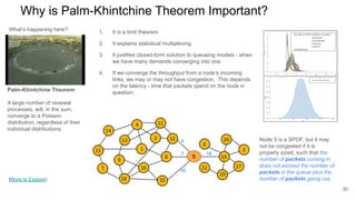
Why is Palm-KhintchineTheorem Important?
What’s happening here?
(More to Explore)
25 sets of 2000 random numbers
Gaussian
Exponential
Gamma
Uniform
distributions
Sum of the 25 sets
Palm-Khintchine Theorem
A large number of renewal
processes, will, in the sum,
converge to a Poisson
distribution, regardless of their
individual distributions.
1. It is a limit theorem
2. It explains statistical multiplexing
3. It justifies closed-form solution to queueing models - when
we have many demands converging into one.
4. If we converge the throughput from a node’s incoming
links, we may or may not have congestion. This depends
on the latency - time that packets spend on the node in
question.
Node 5 is a SPOF, but it may
not be congested if it is
properly sized, such that the
number of packets coming in
does not exceed the number of
packets in the queue plus the
number of packets going out.
5
30
5
7
10
19
31.
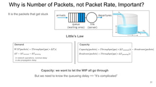
Why is Numberof Packets, not Packet Rate, Important?
It is the packets that get stuck
Little’s Law
Capacity: we want to let the WIP all go through
But we need to know the queueing delay => “It’s complicated”
In network operations, nominal delay
is aka propagation delay
Demand Capacity
31
32.
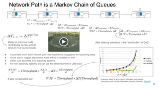
Network Path isa Markov Chain of Queues
A Z
B C ...
Jitter (latency variation) is the “silent killer” of QoS
Delay at previous node
contributes to inter-arrival
time (IAT) at current node
● As packets move down network path, they experience propagation and queueing delay.
● As we saw in Nagoya experiment, there will be a variability in WIP.
● Little’s Law describes it for stationary systems.
● For non-stationary systems, we can use the differential form of Little’s law:
Queueing delay as a function of utilization (normalized
throughput) and number of parallel channels (servers) (Source)
It gets complicated fast
32
33.
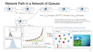
Network Path ina Network of Queues
A Z
B C ...
A’
Now the WIP at node i (here i == C) is the sum of WIPs
coming in and the queueing WIP on node C, which in turn is a
function of total throughput going through node C.
Routing
33
Statmuxing
Queueing delay as a function of utilization (normalized
throughput) and number of parallel channels (servers) (Source)
Queueing
Got to account for statmuxing, queueing, and routing.
34.
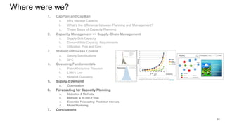
Where were we?
1.CapPlan and CapMan
a. Why Manage Capacity
b. What’s the difference between Planning and Management?
c. Three Steps of Capacity Planning
2. Capacity Management == Supply-Chain Management
a. Supply-Side Capacity
b. Demand-Side Capacity: Requirements
c. Utilization: Pros and Cons
3. Statistical Process Control
a. Setting Specifications
b. SPC
4. Queueing Fundamentals
a. Palm-Khintchine Theorem
b. Little’s Law
c. Network Queueing
5. Supply ≥ Demand
a. Optimization
6. Forecasting for Capacity Planning
a. Motivation & Methods
b. Methods: a 30,000-ft View
c. Ensemble Forecasting: Prediction Intervals
d. Model Monitoring
7. Conclusions
34
35.
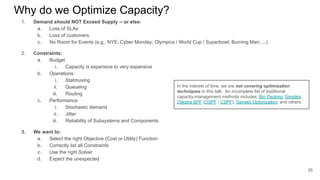
Why do weOptimize Capacity?
1. Demand should NOT Exceed Supply -- or else:
a. Loss of SLAs
b. Loss of customers
c. No Room for Events (e.g., NYE; Cyber Monday; Olympics / World Cup / Superbowl; Burning Man; ...)
2. Constraints:
a. Budget
i. Capacity is expensive to very expensive
b. Operations:
i. Statmuxing
ii. Queueing
iii. Routing
c. Performance:
i. Stochastic demand
ii. Jitter
iii. Reliability of Subsystems and Components
3. We want to:
a. Select the right Objective (Cost or Utility) Function
b. Correctly list all Constraints
c. Use the right Solver
d. Expect the unexpected
35
In the interest of time, we are not covering optimization
techniques in this talk. An incomplete list of traditional
capacity-management methods includes: Bin Packing; Simplex;
Dijkstra SPF (OSPF / CSPF); Genetic Optimization; and others.
36.
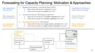
Forecasting for CapacityPlanning: Motivation & Approaches
36
1. Strategic forecasting - Long-Range Plans (LRPs):
a. What will the demand be X years from now?
b. What will the supply be X years from now?
2. Tactical forecasting - Mid-Range (usually PoR)
a. What will the demand be Y months / quarters from now?
b. What will the supply be Y months / quarters from now?
3. Operational forecasting - Short-Range
a. What will the demand be Z days / hours / minutes from now?
b. What will the supply be Z days / hours / minutes from now?
High aggregation;
Low precision
Upper Bound of Demand;
Lower Bound of Supply
High aggregation;
Medium precision
Range of Demand;
Range of Supply
Low aggregation;
High precision
Range of Demand;
Range of Supply
Individual
Entity
Demand
Prediction
Interval
Boundaries
Sum of the
Demand
Probabilistic
Forecast
Hyperparameter
Tuning
Monte-Carlo
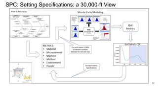
37.
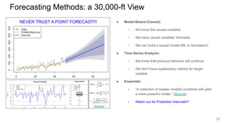
Forecasting Methods: a30,000-ft View
37
(Source)
● Model-Based (Causal):
○ We know the causal variables
○ We have causal variables’ forecasts
○ We can build a causal model (ML or Simulation)
● Time-Series Analysis:
○ We know that previous behavior will continue
○ We don’t have explanatory metrics for target
variable
● Ensemble:
○ “A collection of weaker models combined will yield
a more powerful model.” (Source)
○ Watch out for Prediction Intervals!!!
NEVER TRUST A POINT FORECAST!!!
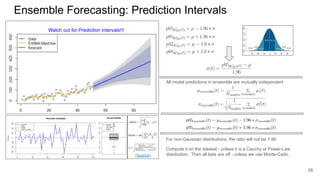
38.
Ensemble Forecasting: PredictionIntervals
38
(Source)
Watch out for Prediction Intervals!!!
For non-Gaussian distributions, the ratio will not be 1.96.
Compute it on the dataset - unless it is a Cauchy or Power-Law
distribution. Then all bets are off - unless we use Monte-Carlo.
All model predictions in ensemble are mutually independent
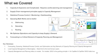
What we Covered
1.Capacity Is Expensive and Complicated. Requires careful planning and management
2. Supply-Chain management principles apply to Capacity Management
3. Statistical Process Control > Monitoring > Dashboarding
4. Queueing Math Works and is Useful
a. Statmuxing
b. Queueing
c. Routing
5. We Optimize Operations and Capacity to keep Supply ≥ Demand
6. Forecasting is a Critical Element of Capacity Planning and Management
40
Key Takeaways:
1. Forecasting, Queueing, Statistical Process Control, and Optimization are Key Elements of Capacity Planning and Capacity Management
2. Local Capacity Management is Meaningless -- Need End to End and Across Layers
3. Capacity Management and Planning relies on models. For models, GIGO is the guiding principle => for CapMan & CapPlan GIGO holds true.