Introduction to Computational Mathematics (2nd Edition, 2015)

October 29, 2014 11:19 BC: 9404 – Intro to Comp Maths 2nd Ed. Yang-Comp-Maths2014 page v
Preface
Computational mathematics is essentially the foundation of modern scien-
tific computing. Traditional ways of doing sciences consist of two major
paradigms: by theory and by experiment. With the steady increase in
computer power, there emerges a third paradigm of doing sciences: by
computer simulation. Numerical algorithms are the very essence of any
computer simulation, and computational mathematics is just the science of
developing and analyzing numerical algorithms.
The science that studies numerical algorithms is numerical analysis or
more broadly computational mathematics. Loosely speaking, numerical
algorithms and analysis should include four categories of algorithms: nu-
merical linear algebra, numerical optimization, numerical solutions of dif-
ferential equations (ODEs and PDEs) and stochastic data modelling.
Many numerical algorithms were developed well before the computer
was invented. For example, Newton’s method for finding roots of nonlinear
equations was developed in 1669, and Gauss quadrature for numerical in-
tegration was formulated in 1814. However, their true power and efficiency
have been demonstrated again and again in modern scientific computing.
Since the invention of the modern computer in the 1940s, many numerical
algorithms have been developed since the 1950s. As the speed of com-
puters increases, together with the increase in the efficiency of numerical
algorithms, a diverse range of complex and challenging problems in math-
ematics, science and engineering can nowadays be solved numerically to
very high accuracy. Numerical algorithms have become more important
than ever.
The topics of computational mathematics are broad and the related
literature is vast. It is often a daunting task for beginners to find the
right book(s) and to learn the right algorithms that are widely used in
v

November 3, 2014 11:34 BC: 9404 – Intro to Comp Maths 2nd Ed. Yang-Comp-Maths2014 page vi
vi Introduction to Computational Mathematics
computational mathematics. Even for lecturers and educators, it is no
trivial task to decide what algorithms to teach and to provide balanced
coverage of a wide range of topics, because there are so many algorithms
to choose from.
The first edition of this book was published by World Scientific Publish-
ing in 2008 and it was well received. Many universities courses used it as
a main reference. Constructive feedbacks and helpful comments have also
been received from the readers. This second edition has incorporated all
these comments and consequently includes more algorithms and new algo-
rithms to reflect the state-of-the-art developments such as computational
intelligence and swarm intelligence.
Therefore, this new edition strives to provide extensive coverage of
efficient algorithms commonly used in computational mathematics and
modern scientific computing. It covers all the major topics including
root-finding algorithms, numerical integration, interpolation, linear algebra,
eigenvalues, numerical methods of ordinary differential equations (ODEs)
and partial differential equations (PDEs), finite difference methods, finite
element methods, finite volume methods, algorithm complexity, optimiza-
tion, mathematical programming, stochastic models such as least squares
and regression, machine learning such as neural networks and support vec-
tor machine, computational intelligence and swarm intelligence such as
cuckoo search, bat algorithm, firefly algorithm as well as particle swarm
optimization.
The book covers both traditional methods and new algorithms with
dozens of worked examples to demonstrate how these algorithms work.
Thus, this book can be used as a textbook and/or reference book, especially
suitable for undergraduates and graduates in computational mathematics,
engineering, computer science, computational intelligence, data science and
scientific computing.
Xin-She Yang
London, 2014

October 29, 2014 11:19 BC: 9404 – Intro to Comp Maths 2nd Ed. Yang-Comp-Maths2014 page vii
Contents
Preface v
I Mathematical Foundations 1
1. Mathematical Foundations 3
1.1 The Essence of an Algorithm . . . . . . . . . . . . . . . . 3
1.2 Big-O Notations . . . . . . . . . . . . . . . . . . . . . . . 5
1.3 Diﬀerentiation and Integration . . . . . . . . . . . . . . . 6
1.4 Vector and Vector Calculus . . . . . . . . . . . . . . . . . 10
1.5 Matrices and Matrix Decomposition . . . . . . . . . . . . 15
1.6 Determinant and Inverse . . . . . . . . . . . . . . . . . . . 20
1.7 Matrix Exponential . . . . . . . . . . . . . . . . . . . . . . 24
1.8 Hermitian and Quadratic Forms . . . . . . . . . . . . . . . 26
1.9 Eigenvalues and Eigenvectors . . . . . . . . . . . . . . . . 28
1.10 Deﬁniteness of Matrices . . . . . . . . . . . . . . . . . . . 31
2. Algorithmic Complexity, Norms and Convexity 33
2.1 Computational Complexity . . . . . . . . . . . . . . . . . 33
2.2 NP-Complete Problems . . . . . . . . . . . . . . . . . . . 34
2.3 Vector and Matrix Norms . . . . . . . . . . . . . . . . . . 35
2.4 Distribution of Eigenvalues . . . . . . . . . . . . . . . . . 37
2.5 Spectral Radius of Matrices . . . . . . . . . . . . . . . . . 44
2.6 Hessian Matrix . . . . . . . . . . . . . . . . . . . . . . . . 47
2.7 Convexity . . . . . . . . . . . . . . . . . . . . . . . . . . . 48
vii

October 29, 2014 11:19 BC: 9404 – Intro to Comp Maths 2nd Ed. Yang-Comp-Maths2014 page viii
viii Introduction to Computational Mathematics
3. Ordinary Differential Equations 51
3.1 Ordinary Differential Equations . . . . . . . . . . . . . . . 51
3.2 First-Order ODEs . . . . . . . . . . . . . . . . . . . . . . 52
3.3 Higher-Order ODEs . . . . . . . . . . . . . . . . . . . . . 53
3.4 Linear System . . . . . . . . . . . . . . . . . . . . . . . . . 56
3.5 Sturm-Liouville Equation . . . . . . . . . . . . . . . . . . 58
4. Partial Differential Equations 59
4.1 Partial Differential Equations . . . . . . . . . . . . . . . . 59
4.1.1 First-Order Partial Differential Equation . . . . . 60
4.1.2 Classification of Second-Order Equations . . . . . 61
4.2 Mathematical Models . . . . . . . . . . . . . . . . . . . . . 61
4.2.1 Parabolic Equation . . . . . . . . . . . . . . . . . 61
4.2.2 Poisson’s Equation . . . . . . . . . . . . . . . . . . 61
4.2.3 Wave Equation . . . . . . . . . . . . . . . . . . . . 62
4.3 Solution Techniques . . . . . . . . . . . . . . . . . . . . . 64
4.3.1 Separation of Variables . . . . . . . . . . . . . . . 65
4.3.2 Laplace Transform . . . . . . . . . . . . . . . . . . 67
4.3.3 Similarity Solution . . . . . . . . . . . . . . . . . . 68
II Numerical Algorithms 71
5. Roots of Nonlinear Equations 73
5.1 Bisection Method . . . . . . . . . . . . . . . . . . . . . . . 73
5.2 Simple Iterations . . . . . . . . . . . . . . . . . . . . . . . 75
5.3 Newton’s Method . . . . . . . . . . . . . . . . . . . . . . . 76
5.4 Iteration Methods . . . . . . . . . . . . . . . . . . . . . . . 78
5.5 Numerical Oscillations and Chaos . . . . . . . . . . . . . . 81
6. Numerical Integration 85
6.1 Trapezium Rule . . . . . . . . . . . . . . . . . . . . . . . . 86
6.2 Simpson’s Rule . . . . . . . . . . . . . . . . . . . . . . . . 87
6.3 Gaussian Integration . . . . . . . . . . . . . . . . . . . . . 89
7. Computational Linear Algebra 95
7.1 System of Linear Equations . . . . . . . . . . . . . . . . . 95
7.2 Gauss Elimination . . . . . . . . . . . . . . . . . . . . . . 97

October 29, 2014 11:19 BC: 9404 – Intro to Comp Maths 2nd Ed. Yang-Comp-Maths2014 page ix
Contents ix
7.3 LU Factorization . . . . . . . . . . . . . . . . . . . . . . . 101
7.4 Iteration Methods . . . . . . . . . . . . . . . . . . . . . . . 103
7.4.1 Jacobi Iteration Method . . . . . . . . . . . . . . . 103
7.4.2 Gauss-Seidel Iteration . . . . . . . . . . . . . . . . 107
7.4.3 Relaxation Method . . . . . . . . . . . . . . . . . 108
7.5 Newton-Raphson Method . . . . . . . . . . . . . . . . . . 109
7.6 QR Decomposition . . . . . . . . . . . . . . . . . . . . . . 110
7.7 Conjugate Gradient Method . . . . . . . . . . . . . . . . . 115
8. Interpolation 117
8.1 Spline Interpolation . . . . . . . . . . . . . . . . . . . . . . 117
8.1.1 Linear Spline Functions . . . . . . . . . . . . . . . 117
8.1.2 Cubic Spline Functions . . . . . . . . . . . . . . . 118
8.2 Lagrange Interpolating Polynomials . . . . . . . . . . . . . 123
8.3 Bézier Curve . . . . . . . . . . . . . . . . . . . . . . . . . 125
III Numerical Methods of PDEs 127
9. Finite Difference Methods for ODEs 129
9.1 Integration of ODEs . . . . . . . . . . . . . . . . . . . . . 129
9.2 Euler Scheme . . . . . . . . . . . . . . . . . . . . . . . . . 130
9.3 Leap-Frog Method . . . . . . . . . . . . . . . . . . . . . . 131
9.4 Runge-Kutta Method . . . . . . . . . . . . . . . . . . . . . 132
9.5 Shooting Methods . . . . . . . . . . . . . . . . . . . . . . 134
10. Finite Difference Methods for PDEs 139
10.1 Hyperbolic Equations . . . . . . . . . . . . . . . . . . . . . 139
10.2 Parabolic Equation . . . . . . . . . . . . . . . . . . . . . . 142
10.3 Elliptical Equation . . . . . . . . . . . . . . . . . . . . . . 143
10.4 Spectral Methods . . . . . . . . . . . . . . . . . . . . . . . 146
10.5 Pattern Formation . . . . . . . . . . . . . . . . . . . . . . 148
10.6 Cellular Automata . . . . . . . . . . . . . . . . . . . . . . 150
11. Finite Volume Method 153
11.1 Concept of the Finite Volume . . . . . . . . . . . . . . . . 153
11.2 Elliptic Equations . . . . . . . . . . . . . . . . . . . . . . . 154
11.3 Parabolic Equations . . . . . . . . . . . . . . . . . . . . . 155
11.4 Hyperbolic Equations . . . . . . . . . . . . . . . . . . . . . 156

October 29, 2014 11:19 BC: 9404 – Intro to Comp Maths 2nd Ed. Yang-Comp-Maths2014 page x
x Introduction to Computational Mathematics
12. Finite Element Method 157
12.1 Finite Element Formulation . . . . . . . . . . . . . . . . . 157
12.1.1 Weak Formulation . . . . . . . . . . . . . . . . . . 157
12.1.2 Galerkin Method . . . . . . . . . . . . . . . . . . . 158
12.1.3 Shape Functions . . . . . . . . . . . . . . . . . . . 159
12.2 Derivatives and Integration . . . . . . . . . . . . . . . . . 163
12.2.1 Derivatives . . . . . . . . . . . . . . . . . . . . . . 163
12.2.2 Gauss Quadrature . . . . . . . . . . . . . . . . . . 164
12.3 Poisson’s Equation . . . . . . . . . . . . . . . . . . . . . . 165
12.4 Transient Problems . . . . . . . . . . . . . . . . . . . . . . 169
IV Mathematical Programming 171
13. Mathematical Optimization 173
13.1 Optimization . . . . . . . . . . . . . . . . . . . . . . . . . 173
13.2 Optimality Criteria . . . . . . . . . . . . . . . . . . . . . . 175
13.3 Unconstrained Optimization . . . . . . . . . . . . . . . . . 177
13.3.1 Univariate Functions . . . . . . . . . . . . . . . . 177
13.3.2 Multivariate Functions . . . . . . . . . . . . . . . 178
13.4 Gradient-Based Methods . . . . . . . . . . . . . . . . . . . 180
13.4.1 Newton’s Method . . . . . . . . . . . . . . . . . . 181
13.4.2 Steepest Descent Method . . . . . . . . . . . . . . 182
14. Mathematical Programming 187
14.1 Linear Programming . . . . . . . . . . . . . . . . . . . . . 187
14.2 Simplex Method . . . . . . . . . . . . . . . . . . . . . . . 189
14.2.1 Basic Procedure . . . . . . . . . . . . . . . . . . . 189
14.2.2 Augmented Form . . . . . . . . . . . . . . . . . . 191
14.2.3 A Case Study . . . . . . . . . . . . . . . . . . . . 192
14.3 Nonlinear Programming . . . . . . . . . . . . . . . . . . . 196
14.4 Penalty Method . . . . . . . . . . . . . . . . . . . . . . . . 196
14.5 Lagrange Multipliers . . . . . . . . . . . . . . . . . . . . . 197
14.6 Karush-Kuhn-Tucker Conditions . . . . . . . . . . . . . . 199
14.7 Sequential Quadratic Programming . . . . . . . . . . . . . 200
14.7.1 Quadratic Programming . . . . . . . . . . . . . . 200
14.7.2 Sequential Quadratic Programming . . . . . . . . 200
14.8 No Free Lunch Theorems . . . . . . . . . . . . . . . . . . 202

October 29, 2014 11:19 BC: 9404 – Intro to Comp Maths 2nd Ed. Yang-Comp-Maths2014 page xi
Contents xi
V Stochastic Methods and Data Modelling 205
15. Stochastic Models 207
15.1 Random Variables . . . . . . . . . . . . . . . . . . . . . . 207
15.2 Binomial and Poisson Distributions . . . . . . . . . . . . . 209
15.3 Gaussian Distribution . . . . . . . . . . . . . . . . . . . . 211
15.4 Other Distributions . . . . . . . . . . . . . . . . . . . . . . 213
15.5 The Central Limit Theorem . . . . . . . . . . . . . . . . . 215
15.6 Weibull Distribution . . . . . . . . . . . . . . . . . . . . . 216
16. Data Modelling 221
16.1 Sample Mean and Variance . . . . . . . . . . . . . . . . . 221
16.2 Method of Least Squares . . . . . . . . . . . . . . . . . . . 223
16.2.1 Maximum Likelihood . . . . . . . . . . . . . . . . 223
16.2.2 Linear Regression . . . . . . . . . . . . . . . . . . 223
16.3 Correlation Coefficient . . . . . . . . . . . . . . . . . . . . 226
16.4 Linearization . . . . . . . . . . . . . . . . . . . . . . . . . 227
16.5 Generalized Linear Regression . . . . . . . . . . . . . . . . 229
16.6 Nonlinear Regression . . . . . . . . . . . . . . . . . . . . . 233
16.7 Hypothesis Testing . . . . . . . . . . . . . . . . . . . . . . 237
16.7.1 Confidence Interval . . . . . . . . . . . . . . . . . 237
16.7.2 Student’s t-Distribution . . . . . . . . . . . . . . . 238
16.7.3 Student’s t-Test . . . . . . . . . . . . . . . . . . . 240
17. Data Mining, Neural Networks and Support Vector Machine 243
17.1 Clustering Methods . . . . . . . . . . . . . . . . . . . . . . 243
17.1.1 Hierarchy Clustering . . . . . . . . . . . . . . . . . 243
17.1.2 k-Means Clustering Method . . . . . . . . . . . . 244
17.2 Artificial Neural Networks . . . . . . . . . . . . . . . . . . 247
17.2.1 Artificial Neuron . . . . . . . . . . . . . . . . . . . 247
17.2.2 Artificial Neural Networks . . . . . . . . . . . . . 248
17.2.3 Back Propagation Algorithm . . . . . . . . . . . . 250
17.3 Support Vector Machine . . . . . . . . . . . . . . . . . . . 251
17.3.1 Classifications . . . . . . . . . . . . . . . . . . . . 251
17.3.2 Statistical Learning Theory . . . . . . . . . . . . . 252
17.3.3 Linear Support Vector Machine . . . . . . . . . . 253
17.3.4 Kernel Functions and Nonlinear SVM . . . . . . . 256

October 29, 2014 11:19 BC: 9404 – Intro to Comp Maths 2nd Ed. Yang-Comp-Maths2014 page xii
xii Introduction to Computational Mathematics
18. Random Number Generators and Monte Carlo Method 259
18.1 Linear Congruential Algorithms . . . . . . . . . . . . . . . 259
18.2 Uniform Distribution . . . . . . . . . . . . . . . . . . . . . 260
18.3 Generation of Other Distributions . . . . . . . . . . . . . . 262
18.4 Metropolis Algorithms . . . . . . . . . . . . . . . . . . . . 266
18.5 Monte Carlo Methods . . . . . . . . . . . . . . . . . . . . 267
18.6 Monte Carlo Integration . . . . . . . . . . . . . . . . . . . 270
18.7 Importance of Sampling . . . . . . . . . . . . . . . . . . . 273
18.8 Quasi-Monte Carlo Methods . . . . . . . . . . . . . . . . . 275
18.9 Quasi-Random Numbers . . . . . . . . . . . . . . . . . . . 276
VI Computational Intelligence 279
19. Evolutionary Computation 281
19.1 Introduction to Evolutionary Computation . . . . . . . . . 281
19.2 Simulated Annealing . . . . . . . . . . . . . . . . . . . . . 282
19.3 Genetic Algorithms . . . . . . . . . . . . . . . . . . . . . . 286
19.3.1 Basic Procedure . . . . . . . . . . . . . . . . . . . 287
19.3.2 Choice of Parameters . . . . . . . . . . . . . . . . 289
19.4 Diﬀerential Evolution . . . . . . . . . . . . . . . . . . . . . 291
20. Swarm Intelligence 295
20.1 Introduction to Swarm Intelligence . . . . . . . . . . . . . 295
20.2 Ant and Bee Algorithms . . . . . . . . . . . . . . . . . . . 296
20.3 Particle Swarm Optimization . . . . . . . . . . . . . . . . 297
20.4 Accelerated PSO . . . . . . . . . . . . . . . . . . . . . . . 299
20.5 Binary PSO . . . . . . . . . . . . . . . . . . . . . . . . . . 301
21. Swarm Intelligence: New Algorithms 303
21.1 Fireﬂy Algorithm . . . . . . . . . . . . . . . . . . . . . . . 303
21.2 Cuckoo Search . . . . . . . . . . . . . . . . . . . . . . . . 306
21.3 Bat Algorithm . . . . . . . . . . . . . . . . . . . . . . . . 310
21.4 Flower Algorithm . . . . . . . . . . . . . . . . . . . . . . . 313
21.5 Other Algorithms . . . . . . . . . . . . . . . . . . . . . . . 317
Bibliography 319
Index 325

October 29, 2014 11:19 BC: 9404 – Intro to Comp Maths 2nd Ed. Yang-Comp-Maths2014 page 1
Part I
Mathematical Foundations

Chapter 1
Mathematical Foundations
Computational mathematics concerns a wide range of topics, from basic
root-finding algorithms and linear algebra to advanced numerical methods
for partial differential equations and nonlinear mathematical programming.
In order to introduce various algorithms, we first review some mathematical
foundations briefly.
1.1 The Essence of an Algorithm
Let us start by asking: what is an algorithm? In essence, an algorithm is
a step-by-step procedure of providing calculations or instructions. Many
algorithms are iterative. The actual steps and procedures will depend on
the algorithm used and the context of interest. However, in this book,
we place more emphasis on iterative procedures and ways for constructing
algorithms.
For example, a simple algorithm of finding the square root of any posi-
tive number k > 0, or x =
√
k, can be written as
xn+1 =
1
2
(xn +
k
xn
), (1.1)
starting from a guess solution x0 = 0, say, x0 = 1. Here, n is the iteration
counter or index, also called the pseudo-time or generation counter. The
above iterative equation comes from the re-arrangement of x2
= k in the
following form
x
2
=
k
2x
, (1.2)
which can be rewritten as
x =
1
2
(x +
k
x
). (1.3)
3

4 Introduction to Computational Mathematics
For example, for k = 7 with x0 = 1, we have
x1 =
1
2
(x0 +
7
x0
) =
1
2
(1 +
7
1
) = 4. (1.4)
x2 =
1
2
(x1 +
7
x1
) = 2.875, x3 ≈ 2.654891304, (1.5)
x4 ≈ 2.645767044, x5 ≈ 2.6457513111. (1.6)
We can see that x5 after just 5 iterations (or generations) is very close to
the true value of
√
7 = 2.64575131106459..., which shows that this iteration
method is very eﬃcient.
The reason that this iterative process works is that the series
x1, x2, ..., xn converges to the true value
√
k due to the fact that
xn+1
xn
=
1
2
(1 +
k
x2
n
) → 1, xn →
√
k, (1.7)
as n → ∞. However, a good choice of the initial value x0 will speed up
the convergence. A wrong choice of x0 could make the iteration fail; for
example, we cannot use x0 = 0 as the initial guess, and we cannot use
x0 < 0 either as
√
k > 0 (in this case, the iterations will approach another
root −
√
k). So a sensible choice should be an educated guess. At the
initial step, if x2
0 < k, x0 is the lower bound and k/x0 is upper bound. If
x2
0 > k, then x0 is the upper bound and k/x0 is the lower bound. For other
iterations, the new bounds will be xn and k/xn. In fact, the value xn+1
is always between these two bounds xn and k/xn, and the new estimate
xn+1 is thus the mean or average of the two bounds. This guarantees that
the series converges to the true value of
√
k. This method is similar to the
well-known bisection method.
You may have already wondered why x2
= k was converted to Eq. (1.1)?
Why do not we write it as the following iterative formula:
xn =
k
xn
, (1.8)
starting from x0 = 1? With this and k = 7, we have
x1 =
7
x0
= 7, x2 =
7
x1
= 1, x3 = 7, x4 = 1, x5 = 7, ..., (1.9)
which leads to an oscillating feature at two distinct stages 1 and 7. You
may wonder that it may be the problem of initial value x0. In fact, for any
initial value x0 = 0, this above formula will lead to the oscillations between
two values: x0 and k. This clearly demonstrates that the way to design a
good iterative formula is very important.

Mathematical Foundations 5
Mathematically speaking, an algorithm A is a procedure to generate a
new and better solution xn+1 to a given problem from the current solution
xn at iteration or time t. That is,
xn+1 = A(xn), (1.10)
where A is a mathematical function of xn. In fact, A can be a set of
mathematical equations in general. In some literature, especially those
in numerical analysis, n is often used for the iteration index. In many
textbooks, the upper index form x(n+1)
or xn+1
is commonly used. Here,
xn+1
does not mean x to the power of n + 1. Such notations will become
useful and no confusion will occur when used appropriately. We will use
such notations when appropriate in this book.
1.2 Big-O Notations
In analyzing the complexity of an algorithm, we usually estimate the order
of computational eﬀorts in terms of its problem size. This often requires
the order notations, often in terms of big O and small o.
Loosely speaking, for two functions f(x) and g(x), if
lim
x→x0
f(x)
g(x)
→ K, (1.11)
where K is a ﬁnite, non-zero limit, we write
f = O(g). (1.12)
The big O notation means that f is asymptotically equivalent to the order
of g(x). If the limit is unity or K = 1, we say f(x) is order of g(x). In this
special case, we write
f ∼ g, (1.13)
which is equivalent to f/g → 1 and g/f → 1 as x → x0. Obviously, x0
can be any value, including 0 and ∞. The notation ∼ does not necessarily
mean ≈ in general, though it may give the same results, especially in the
case when x → 0. For example, sin x ∼ x and sin x ≈ x if x → 0.
When we say f is order of 100 (or f ∼ 100), this does not mean f ≈ 100,
but it can mean that f could be between about 50 and 150. The small o
notation is often used if the limit tends to 0. That is
lim
x→x0
f
g
→ 0, (1.14)

or
f = o(g). (1.15)
If g > 0, f = o(g) is equivalent to f g. For example, for ∀x ∈ R, we
have
ex
≈ 1 + x + O(x2
) ≈ 1 + x +
x2
2
+ o(x).
Example 1.1: A classic example is Stirling’s asymptotic series for facto-
rials
n! ∼
√
2πn (
n
e
)n
(1 +
1
12n
+
1
288n2
−
139
51480n3
− ...),
which can demonstrate the fundamental difference between an asymptotic
series and the standard approximate expansions. For the standard power
expansions, the error Rk(hk
) → 0, but for an asymptotic series, the error
of the truncated series Rk decreases compared with the leading term [here√
2πn(n/e)n
]. However, Rn does not necessarily tend to zero. In fact,
R2 =
1
12n
·
√
2πn(n/e)n
,
is still very large as R2 → ∞ if n 1. For example, for n = 100, we have
n! = 9.3326 × 10157
, while the leading approximation is
√
2πn(n/e)n
=
9.3248 × 10157
. The difference between these two values is 7.7740 × 10154
,
which is still very large, though three orders smaller than the leading ap-
proximation.
1.3 Differentiation and Integration
Differentiation is essentially to find the gradient of a function. For any
curve y = f(x), we define the gradient as
f (x) ≡
dy
dx
≡
df(x)
dx
= lim
h→0
f(x + h) − f(x)
h
. (1.16)
The gradient is also called the first derivative. The three notations f (x),
dy/dx and df(x)/dx are interchangeable. Conventionally, the notation
dy/dx is called Leibnitz’s notation, while the prime notation is called
Lagrange’s notation. Newton’s dot notation ˙y = dy/dt is now exclusively
used for time derivatives. The choice of such notations is purely for clarity,
convention and/or personal preference.

From the basic definition of the derivative, we can verify that differ-
entiation is a linear operator. That is to say that for any two functions
f(x), g(x) and two constants α and β, the derivative or gradient of a linear
combination of the two functions can be obtained by differentiating the
combination term by term. We have
[αf(x) + βg(x)] = αf (x) + βg (x), (1.17)
which can easily be extended to multiple terms.
If y = f(u) is a function of u, and u is in turn a function of x, we want
to calculate dy/dx. We then have
dy
dx
=
dy
du
·
du
dx
, (1.18)
or
df[u(x)]
dx
=
df(u)
du
·
du(x)
dx
. (1.19)
This is the well-known chain rule.
It is straightforward to verify the product rule
(uv) = uv + vu . (1.20)
If we replace v by 1/v = v−1
and apply the chain rule
d(v−1
)
dx
= −1 × v−1−1
×
dv
dx
= −
1
v2
dv
dx
, (1.21)
we have the formula for quotients or the quotient rule
d(u
v )
dx
=
d(uv−1
)
dx
= u(
−1
v2
)
dv
dx
+ v−1 du
dx
=
v du
dx − udv
dx
v2
. (1.22)
For a smooth curve, it is relatively straightforward to draw a tangent
line at any point; however, for a smooth surface, we have to use a tangent
plane. For example, we now want to take the derivative of a function of two
independent variables x and y, that is z = f(x, y) = x2
+y2
/2. The question
is probably ‘with respect to’ what? x or y? If we take the derivative with
respect to x, then will it be affected by y? The answer is we can take
the derivative with respect to either x or y while taking the other variable
as constant. That is, we can calculate the derivative with respect to x in
the usual sense by assuming that y = constant. Since there is more than
one variable, we have more than one derivative and the derivatives can be
associated with either the x-axis or y-axis. We call such derivatives partial
derivatives, and use the following notation
∂z
∂x
≡
∂f(x, y)
∂x
≡ fx ≡
∂f
∂x y
= lim
h→0,y=const
f(x + h, y) − f(x, y)
h
. (1.23)

The notation ∂f
∂x |y emphasises the fact that y = constant; however, we often
omit |y and simply write ∂f
∂x as we know this fact is implied.
Similarly, the partial derivative with respect to y is defined by
∂z
∂y
≡
∂f(x, y)
∂y
≡ fy ≡
∂f
∂y x
= lim
x=const,k→0
f(x, y + k) − f(x, y)
k
. (1.24)
Then, the standard differentiation rules for univariate functions such as
f(x) apply. For example, for z = f(x, y) = x2
+ y2
/2, we have
∂f
∂x
=
dx2
dx
+ 0 = 2x,
and
∂f
∂y
= 0 +
d(y2
/2)
dy
=
1
2
× 2y = y,
where the appearance of 0 highlights the fact that dy/dx = dx/dy = 0 as
x and y are independent variables.
Differentiation is used to find the gradient for a given function. Now a
natural question is how to find the original function for a given gradient.
This is the integration process, which can be considered as the reverse of
the differentiation process. Since we know that
d sin x
dx
= cos x, (1.25)
that is, the gradient of sin x is cos x, we can easily say that the original
function is sin x since its gradient is cos x. We can write
cos x dx = sin x + C, (1.26)
where C is the constant of integration. Here dx is the standard notation
showing the integration is with respect to x, and we usually call this the
integral. The function cos x is called the integrand.
The integration constant comes from the fact that a family of curves
shifted by a constant will have the same gradient at their corresponding
points. This means that the integration can be determined up to an arbi-
trary constant. For this reason, we call it an indefinite integral.
Integration is more complicated than differentiation in general. Even
when we know the derivative of a function, we have to be careful. For
example, we know that (xn+1
) = (n + 1)xn
or ( 1
n+1 xn+1
) = xn
for any n
integers, so we can write
xn
dx =
1
n + 1
xn+1
+ C. (1.27)

However, there is a possible problem when n = −1 because 1/(n + 1) will
become 1/0. In fact, the above integral is valid for any n except n = −1.
When n = −1, we have
1
x
dx = ln x + C. (1.28)
If we know that the gradient of a function F(x) is f(x) or F (x) = f(x),
it is possible and sometimes useful to express where the integration starts
and ends, and we often write
b
a
f(x)dx = F(x)
b
a
= F(b) − F(a). (1.29)
Here a is called the lower limit of the integral, while b is the upper limit
of the integral. In this case, the constant of integration has dropped out
because the integral can be determined accurately. The integral becomes a
deﬁnite integral and it corresponds to the area under a curve f(x) from a
to b ≥ a.
From the diﬀerentiation rule
d(uv)
dx
= u
dv
dx
+ v
du
dx
, (1.30)
we integrate it with respect to x, we have
d(uv)
dx
dx = uv = u
dv
dx
dx + v
du
dx
dx. (1.31)
By rearranging, we have
u
dv
dx
dx = uv − v
du
dx
dx, (1.32)
or
uv dx = uv − vu dx, (1.33)
or simply
udv = uv − vdu. (1.34)
This is the well-known formula for the technique known as integration by
parts.
Example 1.2: To calculate xex
dx, we can set u = x and v = ex
, which
gives u = 1 and v = ex
. Now we have
xex
dx = xex
− ex
· 1dx = xex
− ex
+ C.
However, this will not work if we set u = ex
and v = x. Thus, care should
be taken when using integration by parts.
Obviously, there are many other techniques for integration such as sub-
stitution and transformation. Integration can also be multivariate, which
leads to multiple integrals. We will not discuss this further, and interested
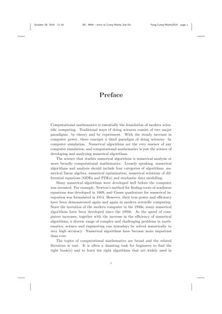
readers can refer to more advanced textbooks.

1.4 Vector and Vector Calculus
Vector analysis is an important part of computational mathematics. Many
quantities such as force, velocity, and deformation in sciences are vectors
which have both a magnitude and a direction. Vectors are a special class of
matrices. Here, we will brieﬂy review the basic concepts in linear algebra.
A vector u is a set of ordered numbers u = (u1, u2, ..., un), where its
components ui(i = 1, ..., n) ∈ are real numbers. All these vectors form
an n-dimensional vector space Vn
. A simple example is the position vector
p = (x, y, z) where x, y, z are the 3-D Cartesian coordinates.
To add any two vectors u = (u1, ..., un) and v = (v1, ..., vn), we simply
add their corresponding components,
u + v = (u1 + v1, u2 + v2, ..., un + vn), (1.35)
and the sum is also a vector. The addition of vectors has commutability
(u + v = v + u) and associativity [(u + v) + w = u + (v + w)]. This
is because each of the components is obtained by simple addition, which
means it has the same properties.
u
v
w
b
v
u
a v
u
Fig. 1.1 Addition of vectors: (a) parallelogram a = u + v; (b) vector polygon b =
u + v + w.
The zero vector 0 is a special case where all its components are zeros.
The multiplication of a vector u with a scalar or constant α ∈ is carried
out by the multiplication of each component,
αu = (αu1, αu2, ..., αun). (1.36)
Thus, we have
−u = (−u1, −u2, ..., −un). (1.37)
The dot product or inner product of two vectors x and y is deﬁned as
x · y = x1y1 + x2y2 + ... + xnyn =
n
i=1
xiyi, (1.38)

which is a real number. The length or norm of a vector x is the root of the
dot product of the vector itself,
|x| = x =
√
x · x =
n
i=1
x2
i . (1.39)
When x = 1, then it is a unit vector. It is straightforward to check that
the dot product has the following properties:
u · v = v · u, u · (v + w) = u · v + u · w, (1.40)
and
(αu) · (βv) = (αβ)u · v, (1.41)
where α, β ∈ are constants.
The angle θ between two vectors u and v can be calculated using their
dot product
u · v = ||u|| ||v|| cos(θ), 0 ≤ θ ≤ π, (1.42)
which leads to
cos(θ) =
u · v
u v
. (1.43)
If the dot product of these two vectors is zero or cos(θ) = 0 (i.e., θ = π/2),
then we say that these two vectors are orthogonal.
Since cos(θ) ≤ 1, then we get the useful Cauchy-Schwartz inequality:
u · v ≤ u v . (1.44)
The dot product of two vectors is a scalar or a number. On the other
hand, the cross product or outer product of two vectors is a new vector
u = x × y =
i j k
x1 x2 x3
y1 y2 y3
=
x2 x3
y2 y3
i +
x3 x1
y3 y1
j +
x1 x2
y1 y2
k
= (x2y3 − x3y2)i + (x3y1 − x1y3)j + (x1y2 − x2y1)k. (1.45)
In fact, the norm of x × y is the area of the parallelogram formed by x
and y. We have
x × y = x y sin θ, (1.46)

where θ is the angle between the two vectors. In addition, the vector
u = x × y is perpendicular to both x and y, following a right-hand rule.
It is straightforward to check that the cross product has the following
properties:
x × y = −y × x, (x + y) × z = x × z + y × z, (1.47)
and
(αx) × (βy) = (αβ)x × y, α, b ∈ . (1.48)
A very special case is u × u = 0. For unit vectors, we have
i × j = k, j × k = i, k × i = j. (1.49)
Example 1.3: For two 3-D vectors u = (4, 5, −6) and v = (2, −2, 1/2),
their dot product is
u · v = 4 × 2 + 5 × (−2) + (−6) × 1/2 = −5.
As their moduli are
||u|| = 42 + 52 + (−6)2 =
√
77,
||v|| = 22 + (−2)2 + (1/2)2 =
√
33/2,
we can calculate the angle θ between the two vectors. We have
cos θ =
u · v
||u||||v||
=
−5
√
77 ×
√
33/2
= −
10
11
√
21
,
or
θ = cos−1
(−
10
11
√
21
) ≈ 101.4◦
.
Their cross product is
w = u × v
= (5 × 1/2 − (−2) × (−6), (−6) × 2 − 4 × 1/2, 4 × (−2) − 5 × 2)
= (−19/2, −14, −18).
Similarly, we have
v × u = (19/2, 14, 18) = −u × v.
The norm of the cross product is
w = (
−19
2
)2 + (−14)2 + (−18)2 ≈ 24.70,

while
u v sin θ =
√
77 ×
√
33
2
× sin(101.4◦
) ≈ 24.70 = w .
It is easy to verify that
u · w = 4 × (−19/2) + 5 × (−14) + (−6) × (−18) = 0,
and
v · w = 2 × (−19/2) + (−2) × (−14) + 1/2 × (−18) = 0.
Indeed, the vector w is perpendicular to both u and v.
Any vector v in an n-dimensional vector space Vn
can be written as a
combination of a set of n independent basis vectors or orthogonal spanning
vectors e1, e2, ..., en, so that
v = v1e1 + v2e2 + ... + vnen =
n
i=1
viei, (1.50)
where the coefficients/scalars v1, v2, ..., vn are the components of v relative
to the basis e1, e2, ..., en. The most common basis vectors are the orthog-
onal unit vectors. In a three-dimensional case, they are i = (1, 0, 0), j =
(0, 1, 0), k = (0, 0, 1) for x-, y-, z-axis, respectively. Thus, we have
x = x1i + x2j + x3k. (1.51)
The three unit vectors satisfy i · j = j · k = k · i = 0.
Two non-zero vectors u and v are said to be linearly independent if
αu + βv = 0 implies that α = β = 0. If α, β are not all zeros, then
these two vectors are linearly dependent. Two linearly dependent vectors
are parallel (u//v) to each other. Similarly, any three linearly dependent
vectors u, v, w are in the same plane.
The differentiation of a vector is carried out over each component and
treating each component as the usual differentiation of a scalar. Thus, from
a position vector
P (t) = x(t)i + y(t)j + z(t)k, (1.52)
we can write its velocity as
v =
dP
dt
= ˙x(t)i + ˙y(t)j + ˙z(t)k, (1.53)
and acceleration as
a =
d2
P
dt2
= ¨x(t)i + ÿ(t)j + ¨z(t)k, (1.54)

where ˙= d/dt. Conversely, the integral of v is
P =
t
0
vdt + p0, (1.55)
where p0 is a vector constant or the initial position at t = 0.
From the basic definition of differentiation, it is easy to check that the
differentiation of vectors has the following properties:
d(αa)
dt
= α
da
dt
,
d(a · b)
dt
=
da
dt
· b + a ·
db
dt
, (1.56)
and
d(a × b)
dt
=
da
dt
× b + a ×
db
dt
. (1.57)
Three important operators commonly used in vector analysis, especially
in the formulation of mathematical models, are the gradient operator (grad
or ∇), the divergence operator (div or ∇·) and the curl operator (curl or
∇×).
Sometimes, it is useful to calculate the directional derivative of φ at a
point (x, y, z) in the direction of n
∂φ
∂n
= n · ∇φ =
∂φ
∂x
cos(α) +
∂φ
∂y
cos(β) +
∂φ
∂z
cos(γ), (1.58)
where n = (cos α, cos β, cos γ) is a unit vector and α, β, γ are the directional
angles. Generally speaking, the gradient of any scalar function φ of x, y, z
can be written in a similar way,
gradφ = ∇φ =
∂φ
∂x
i +
∂φ
∂y
j +
∂φ
∂z
k. (1.59)
This is the same as the application of the del operator ∇ to the scalar
function φ
∇ =
∂
∂x
i +
∂
∂y
j +
∂
∂z
k. (1.60)
The direction of the gradient operator on a scalar field gives a vector field.
As the gradient operator is a linear operator, it is straightforward to
check that it has the following properties:
∇(αψ + βφ) = α∇ψ + β∇φ, ∇(ψφ) = ψ∇φ + φ∇ψ, (1.61)
where α, β are constants and ψ, φ are scalar functions.
For a vector field
u(x, y, z) = u(x, y, z)i + v(x, y, z)j + w(x, y, z)k, (1.62)

the application of the operator ∇ can lead to either a scalar field or vector
field depending on how the del operator is applied to the vector field. The
divergence of a vector field is the dot product of the del operator ∇ and u
div u ≡ ∇ · u =
∂u1
∂x
+
∂u2
∂y
+
∂u3
∂z
, (1.63)
and the curl of u is the cross product of the del operator and the vector
field u
curl u ≡ ∇ × u =
i j k
∂
∂x
∂
∂y
∂
∂z
u1 u2 u3
. (1.64)
One of the most commonly used operators in engineering and science is
the Laplacian operator
∇2
φ = ∇ · (∇φ) =
∂2
φ
∂x2
+
∂2
φ
∂y2
+
∂2
φ
∂z2
, (1.65)
for Laplace’s equation
Δφ ≡ ∇2
φ = 0. (1.66)
Some important theorems are often rewritten in terms of the above
three operators, especially in fluid dynamics and finite element analysis.
For example, Gauss’s theorem connects the integral of divergence with the
related surface integral
Ω
(∇ · Q) dΩ =
S
Q · n dS. (1.67)
1.5 Matrices and Matrix Decomposition
Matrices are widely used in scientific computing, engineering and sciences,
especially in the implementation of many algorithms. A matrix is a table or
array of numbers or functions arranged in rows and columns. The elements
or entries of a matrix A are often denoted as aij. For a matrix A with m
rows and n columns,
A ≡ [aij] =
⎛
⎜
⎜
⎜
⎝
a11 a12 ... a1j ... a1n
a21 a22 ... a2j ... a2n
...
...
...
...
am1 am2 ... amj ... amn
⎞
⎟
⎟
⎟
⎠
, (1.68)

we say the size of A is m by n, or m × n. A is a square matrix if m = n.
For example,
A =
1 2 3
4 5 6
, B =
ex
sin x
−i cosx eiθ , (1.69)
and
u =
⎛
⎝
u
v
w
⎞
⎠, (1.70)
where A is a 2 × 3 matrix, B is a 2 × 2 square matrix, and u is a 3 × 1
column matrix or column vector.
The sum of two matrices A and B is possible only if they have the same
size m × n, and their sum, which is also m × n, is obtained by adding their
corresponding entries
C = A + B, cij = aij + bij, (1.71)
where (i = 1, 2, ..., m; j = 1, 2, ..., n). The product of a matrix A with a
scalar α ∈ is obtained by multiplying each entry by α. The product of
two matrices is possible only if the number of columns of A is the same as
the number of rows of B. That is to say, if A is m× n and B is n× r, then
the product C is m × r,
cij = (AB)ij =
n
k=1
aikbkj. (1.72)
If A is a square matrix, then we have An
=
n
AA...A. The multiplications
of matrices are generally not commutive, i.e., AB = BA. However, the
multiplication has associativity A(uv) = (Au)v and A(u+v) = Au+Av.
The transpose AT
of A is obtained by switching the position of rows
and columns, and thus AT
will be n × m if A is m × n, (aT
)ij = aji, (i =
1, 2, ..., m; j = 1, 2, ..., n). Generally,
(AT
)T
= A, (AB)T
= BT
AT
. (1.73)
The diﬀerentiation and integral of a matrix are carried out over each of
its members or elements. For example, for a 2 × 2 matrix
dA
dt
= ˙A =
⎛
⎝
da11
dt
da12
dt
da21
dt
da22
dt
⎞
⎠, (1.74)

and
Adt =
⎛
⎝
a11dt a12dt
a21dt a22dt
⎞
⎠. (1.75)
A diagonal matrix A is a square matrix whose every entry off the main
diagonal is zero (aij = 0 if i = j). Its diagonal elements or entries may or
may not have zeros. In general, it can be written as
D =
⎛
⎜
⎜
⎜
⎝
d1 0 ... 0
0 d2 ... 0
...
0 0 ... dn
⎞
⎟
⎟
⎟
⎠
. (1.76)
For example, the matrix
I =
⎛
⎝
1 0 0
0 1 0
0 0 1
⎞
⎠ (1.77)
is a 3 × 3 identity or unitary matrix. In general, we have
AI = IA = A. (1.78)
A zero or null matrix 0 is a matrix with all of its elements being zero.
There are three important matrices: lower (upper) triangular matrix,
tridiagonal matrix, and augmented matrix, and they are important in the
solution of linear equations. A tridiagonal matrix often arises naturally
from the finite difference and finite volume discretization of partial differ-
ential equations, and it can in general be written as
Q =
⎛
⎜
⎜
⎜
⎜
⎜
⎝
b1 c1 0 0 ... 0 0
a2 b2 c2 0 ... 0 0
0 a3 b3 c3 ... 0 0
...
...
...
0 0 0 0 ... an bn
⎞
⎟
⎟
⎟
⎟
⎟
⎠
. (1.79)
An augmented matrix is formed by two matrices with the same number
of rows. For example, the following system of linear equations
a11u1 + a12u2 + a13u3 = b1,
a21u1 + a22u2 + a23u3 = b2,
a31u1 + a32u2 + a33u3 = b3, (1.80)

November 3, 2014 11:34 BC: 9404 – Intro to Comp Maths 2nd Ed. Yang-Comp-Maths2014 page 18
can be written in a compact form in terms of matrices
⎛
⎝
a11 a12 a13
a21 a22 a23
a31 a32 a33
⎞
⎠
⎛
⎝
u1
u2
u3
⎞
⎠ =
⎛
⎝
b1
b2
b3
⎞
⎠, (1.81)
or
Au = b. (1.82)
This can in turn be written as the following augmented form
[A|b] =
⎛
⎝
a11 a12 a13 b1
a21 a22 a23 b2
a31 a32 a33 b3
⎞
⎠ . (1.83)
The augmented form is widely used in Gauss-Jordan elimination and linear
programming.
A lower (upper) triangular matrix is a square matrix with all the ele-
ments above (below) the diagonal entries being zeros. In general, a lower
triangular matrix can be written as
L =
⎛
⎜
⎜
⎜
⎝
l11 0 ... 0
l21 l22 ... 0
...
ln1 ln2 ... lnn
⎞
⎟
⎟
⎟
⎠
, (1.84)
while the upper triangular matrix can be written as
U =
⎛
⎜
⎜
⎜
⎝
u11 u12 ... u1n
0 u22 ... u2n
...
0 0 ... unn
⎞
⎟
⎟
⎟
⎠
. (1.85)
Any n × n square matrix A = [aij] can be decomposed or factorized as a
product of an L and a U, that is
A = LU, (1.86)
though some decomposition is not unique because we have n2
+n unknowns:
n(n + 1)/2 coefficients lij and n(n + 1)/2 coefficients uij, but we can only
provide n2
equations from the coefficients aij. Thus, there are n free pa-
rameters. The uniqueness of decomposition is often achieved by imposing
either lii = 1 or uii = 1 where i = 1, 2, ..., n.
Other LU variants include the LDU and LUP decompositions. An LDU
decomposition can be written as
A = LDU, (1.87)

where L and U are lower and upper matrices with all the diagonal entries
being unity, and D is a diagonal matrix. On the other hand, the LUP
decomposition can be expressed as
A = LUP , or A = P LU, (1.88)
where P is a permutation matrix which is a square matrix and has exactly
one entry 1 in each column and each row with 0’s elsewhere. However, most
numerical libraries and software packages use the following LUP decompo-
sition
P A = LU, (1.89)
which makes it easier to decompose some matrices. However, the require-
ment for LU decompositions is relatively strict. An invertible matrix A
has an LU decomposition provided that the determinants of all its diagonal
minors or leading submatrices are not zeros.
A simpler way of decomposing a square matrix A for solving a system
of linear equations is to write
A = D + L + U, (1.90)
where D is a diagonal matrix. L and U are the strictly lower and upper
triangular matrices without diagonal elements, respectively. This decom-
position is much simpler to implement than the LU decomposition because
there is no multiplication involved here.
Example 1.4: The following 3 × 3 matrix
A =
⎛
⎝
2 1 5
4 −4 5
5 2 −5
⎞
⎠,
can be decomposed as A = LU. That is
A =
⎛
⎝
1 0 0
l21 1 0
l31 l32 0
⎞
⎠
⎛
⎝
u11 u12 u13
0 u22 u23
0 0 u33
⎞
⎠,
which becomes
A =
⎛
⎝
u11 u12 u13
l21u11 l21u12 + u22 l21u13 + u23
l31u11 l31u12 + l32u22 l31u13 + l32u23 + u33
⎞
⎠
=
⎛
⎝
2 1 5
4 −4 5
5 2 −5
⎞
⎠.

This leads to u11 = 2, u12 = 1 and u13 = 5. As l21u11 = 4, so l21 =
4/u11 = 2. Similarly, l31 = 2.5. From l21u12 + u22 = −4, we have u22 =
−4 − 2 × 1 = −6. From l21u13 + u23 = 5, we have u23 = 5 − 2 × 5 = −5.
Using l31u12 +l32u22 = 2, or 2.5×1+l32 ×(−6) = 2, we get l32 = 1/12.
Finally, l31u13 +l32u23 +u33 = −5 gives u33 = −5−2.5×5−1/12×(−5) =
−205/12. Therefore, we now have
⎛
⎝
2 1 5
4 −4 5
5 2 −5
⎞
⎠ =
⎛
⎝
1 0 0
2 1 0
5/2 1/12 1
⎞
⎠
⎛
⎝
2 1 5
0 −6 −5
0 0 −205/12
⎞
⎠.
The L+D+U decomposition can be written as
A = D + L + U =
⎛
⎝
2 0 0
0 −4 0
0 0 −5
⎞
⎠ +
⎛
⎝
0 0 0
4 0 0
5 2 0
⎞
⎠ +
⎛
⎝
0 1 5
0 0 5
0 0 0
⎞
⎠.
1.6 Determinant and Inverse
The determinant of a square matrix A is a number or scalar obtained by
the following recursive formula, or the cofactors, or the Laplace expansion
by column or row. For example, expanding by row k, we have
det(A) = |A| =
n
j=1
(−1)k+j
akjMkj, (1.91)
where Mij is the determinant of a minor matrix of A by deleting row i and
column j. For a simple 2 × 2 matrix, its determinant simply becomes
a11 a12
a21 a22
= a11a22 − a12a21. (1.92)
The determinants of matrices have the following properties:
|αA| = α|A|, |AT
| = |A|, |AB| = |A||B|, (1.93)
where A and B have the same size (n × n).
An n × n square matrix is singular if |A| = 0, and is nonsingular if and
only if |A| = 0. The trace of a square matrix tr(A) is deﬁned as the sum
of the diagonal elements,
tr(A) =
n
i=1
aii = a11 + a22 + ... + ann. (1.94)

The rank of a matrix A is the number of linearly independent vectors
forming the matrix. Generally speaking, the rank of A satisfies
rank(A) ≤ min(m, n). (1.95)
For an n × n square matrix A, it is nonsingular if rank(A) = n.
The inverse matrix A−1
of a square matrix A is defined as
A−1
A = AA−1
= I. (1.96)
More generally,
A−1
l A = AA−1
r = I, (1.97)
where A−1
l is the left inverse while A−1
r is the right inverse. If A−1
l = A−1
r ,
we say that the matrix A is invertible and its inverse is simply denoted by
A−1
. It is worth noting that the unit matrix I has the same size as A.
The inverse of a square matrix exists if and only if A is nonsingular or
det(A) = 0. From the basic definitions, it is straightforward to prove that
the inverse of a matrix has the following properties
(A−1
)−1
= A, (AT
)−1
= (A−1
)T
, (1.98)
and
(AB)−1
= B−1
A−1
. (1.99)
The inverse of a lower (upper) triangular matrix is also a lower (upper)
triangular matrix. The inverse of a diagonal matrix
D =
⎛
⎜
⎜
⎜
⎝
d1 0 ... 0
0 d2 ... 0
...
0 0 ... dn
⎞
⎟
⎟
⎟
⎠
, (1.100)
can simply be written as
D−1
=
⎛
⎜
⎜
⎜
⎝
1/d1 0 ... 0
0 1/d2 ... 0
...
0 0 ... 1/dn
⎞
⎟
⎟
⎟
⎠
, (1.101)
where di = 0. If any of these elements di is zero, then the diagonal matrix
is not invertible as it becomes singular. For a 2 × 2 matrix, its inverse is
simply
A =
a b
c d
, A−1
=
1
ad − bc
d −b
−c a
. (1.102)

Example 1.5: For two matrices,
A =
⎛
⎝
4 5 0
−2 2 5
2 −3 1
⎞
⎠, B =
⎛
⎝
2 3
0 −2
5 2
⎞
⎠,
their transpose matrices are
AT
=
⎛
⎝
4 −2 2
5 2 −3
0 5 1
⎞
⎠, BT
=
2 0 5
3 −2 2
.
Let D = AB be their product; we have
AB = D =
⎛
⎝
D11 D12
D21 D22
D31 D32
⎞
⎠.
The ﬁrst two entries are
D11 =
3
j=1
A1jBj1 = 2 × 4 + 5 × 0 + 0 × 5 = 8,
and
D12 =
3
j=1
A1jBj2 = 4 × 3 + 5 × (−2) + 0 × 2 = 2.
Similarly, the other entries are:
D21 = 21, D22 = 0, D31 = 9, D33 = 14.
Therefore, we get
AB =
⎛
⎝
4 5 0
−2 2 5
2 −3 1
⎞
⎠
⎛
⎝
2 3
0 −2
5 2
⎞
⎠ = D =
⎛
⎝
8 2
21 0
9 14
⎞
⎠.
However, the product BA does not exist, though
BT
AT
=
8 21 9
2 0 14
= DT
= (AB)T
.
The inverse of A is
A−1
=
1
128
⎛
⎝
17 −5 25
12 4 −20
2 22 18
⎞
⎠,

and the determinant of A is
det(A) = 128.
It is straightforward to verify that
AA−1
= A−1
A = I =
⎛
⎝
1 0 0
0 1 0
0 0 1
⎞
⎠.
For example, the first entry is obtained by
3
j=1
A1jA−1
j1 = 4 ×
17
128
+ 5 ×
12
128
+ 0 ×
2
128
= 1.
Other entries can be verified similarly. Finally, the trace of A is
tr(A) = A11 + A22 + A33 = 4 + 2 + 1 = 7.
The algorithmic complexity of most algorithms for obtaining the inverse
of a general square matrix is O(n3
). That is why most modern algorithms
try to avoid the direct inverse of a large matrix. Solution of a large matrix
system is instead carried out either by partial inverse via decomposition
or by iteration (or a combination of these two methods). If the matrix
can be decomposed into triangular matrices either by LU factorization or
direction decomposition, the aim is then to invert a triangular matrix, which
is simpler and more efficient.
For a triangular matrix, the inverse can be obtained using algorithms
of O(n2
) complexity. Similarly, the solution of a linear system with a lower
(upper) triangular matrix A can be obtained by forward (back) substitu-
tions. In general, for a lower triangular matrix
A =
⎛
⎜
⎜
⎜
⎝
α11 0 ... 0
α12 α22 ... 0
...
αn1 αn2 ... αnn
⎞
⎟
⎟
⎟
⎠
, (1.103)
the forward substitutions for the system Au = b can be carried out as
follows:
u1 =
b1
α11
,
u2 =
1
α22
(b2 − α21u1),

ui =
1
αii
(bi −
i−1
j=1
αijuj), (1.104)
where i = 2, ..., n. We see that it takes 1 division to get u1, 3 floating
point calculations to get u2, and (2i− 1) to get ui. So the total algorithmic
complexity is O(1 + 3 + ... + (2n − 1)) = O(n2
). Similar arguments apply
to the upper triangular systems.
The inverse A−1
of a lower triangular matrix can in general be written
as
A−1
=
⎛
⎜
⎜
⎜
⎝
β11 0 ... 0
β21 β22 ... 0
...
βn1 βn2 ... βnn
⎞
⎟
⎟
⎟
⎠
= B = B1 B2 ... Bn , (1.105)
where Bj are the j-th column vector of B. The inverse must satisfy
AA−1
= I or
A B1 B2 ... Bn = I = e1 e2 ... en , (1.106)
where ej is the j-th unit vector of size n with the j-th element being 1 and
all other elements being zero. That is eT
j = 0 0 ... 1 0 ... 0 . In order to
obtain B, we have to solve n linear systems
AB1 = e1, AB2 = e2, ..., ABn = en. (1.107)
As A is a lower triangular matrix, the solution of ABj = ej can easily be
obtained by direct forward substitutions discussed earlier in this section.
1.7 Matrix Exponential
Sometimes, we need to calculate exp[A], where A is a square matrix. In
this case, we have to deal with matrix exponentials. The exponential of a
square matrix A is defined as
eA ≡
∞
n=0
1
n!
An
= I + A +
1
2!
A2
+ ..., (1.108)
where I is an identity matrix with the same size as A, and A2
= AA and
so on. This (rather odd) definition in fact provides a method of calculating

the matrix exponential. The matrix exponentials are very useful in solving
systems of diﬀerential equations.
Example 1.6: For a simple matrix
A =
t 0
0 t
,
its exponential is simply
eA =
et
0
0 et .
For a more complicated matrix
B =
t a
a t
,
we have
eB =
⎛
⎝
1
2 (et+a
+ et−a
) 1
2 (et+a
− et−a
)
1
2 (et+a
− et−a
) 1
2 (et+a
+ et−a
)
⎞
⎠.
As you can see, it is quite complicated but still straightforward to cal-
culate the matrix exponentials. Fortunately, it can easily be done using
most computer software packages. By using the power expansions and the
basic deﬁnition, we can prove the following useful identities
etA ≡
∞
n=0
1
n!
(tA)n
= I + tA +
t2
2!
A2
+ ..., (1.109)
ln(I + A) ≡
∞
n=1
(−1)n−1
n!
An
= A −
1
2
A2
+
1
3
A3
+ ..., (1.110)
eAeB = eA+B (if AB = BA), (1.111)
d
dt
(etA) = AetA = etAA, (1.112)
(eA)−1
= e−A, det(eA) = etrA. (1.113)

1.8 Hermitian and Quadratic Forms
The matrices we have discussed so far are real matrices because all their
elements are real. In general, the entries or elements of a matrix can be
complex numbers, and the matrix becomes a complex matrix. For a matrix
A, its complex conjugate A∗
is obtained by taking the complex conjugate
of each of its elements. The Hermitian conjugate A†
is obtained by taking
the transpose of its complex conjugate matrix. That is to say, for
A =
⎛
⎝
a11 a12 ...
a21 a21 ...
... ... ...
⎞
⎠, (1.114)
we have
A∗
=
⎛
⎝
a∗
11 a∗
12 ...
a∗
21 a∗
22 ...
... ... ...
⎞
⎠, (1.115)
and
A†
= (A∗
)T
= (AT
)∗
=
⎛
⎝
a∗
11 a∗
21 ...
a∗
12 a22 ...
... ... ...
⎞
⎠. (1.116)
A square matrix A is called orthogonal if and only if A−1
= AT
. If a
square matrix A satisﬁes A∗
= A, it is called an Hermitian matrix. It is
an anti-Hermitian matrix if A∗
= −A. If the Hermitian matrix of a square
matrix A is equal to the inverse of the matrix (or A†
= A−1
), it is called
a unitary matrix.
Example 1.7: For a complex matrix
A =
2 + 3iπ 1 + 9i 0
eiπ
−2i i sin θ
,
its complex conjugate A∗
is
A∗
=
2 − 3iπ 1 − 9i 0
e−iπ
2i −i sin θ
.
The Hermitian conjugate of A is
A†
=
⎛
⎝
2 − 3iπ e−iπ
1 − 9i 2i
0 −i sinθ
⎞
⎠ = (A∗
)T
.

For the rotation matrix
A =
cos θ sin θ
− sin θ cos θ
,
its inverse and transpose are
A−1
=
1
cos2 θ + sin2
θ
cos θ − sin θ
sin θ cos θ
,
and
AT
=
cos θ − sin θ
sin θ cos θ
.
Since cos2
θ + sin2
θ = 1, we have AT
= A−1
. Therefore, the original
rotation matrix A is orthogonal.
A very useful concept in computational mathematics and computing
is quadratic forms. For a real vector qT
= (q1, q2, q3, ..., qn) and a real
symmetric square matrix A, a quadratic form ψ(q) is a scalar function
deﬁned by
ψ(q) = qT
Aq = q1 q2 ... qn
⎛
⎜
⎜
⎝
A11 A12 ... A1n
A21 A22 ... A2n
... ... ... ...
An1 An2 ... Ann
⎞
⎟
⎟
⎠
⎛
⎜
⎜
⎜
⎝
q1
q2
...
qn
⎞
⎟
⎟
⎟
⎠
, (1.117)
which can be written as
ψ(q) =
n
i=1
n
j=1
qiAijqj. (1.118)
Since ψ is a scalar, it should be independent of the coordinates.
In the case of a square matrix A, ψ might be more easily evaluated in
certain intrinsic coordinates Q1, Q2, ..., Qn. An important result concerning
the quadratic form is that it can always be written through appropriate
transformations as
ψ(q) =
n
i=1
λiQ2
i = λ1Q2
1 + λ2Q2
2 + ... + λnQ2
n, (1.119)
where λi are the eigenvalues of the matrix A determined by
det |A − λI| = 0, (1.120)
and Qi are the intrinsic components along directions of the eigenvectors in
this case.

The natural extension of quadratic forms is the Hermitian form which
is the quadratic form for a complex Hermitian matrix A. Furthermore,
the matrix A can consist of linear operators and functionals in addition to
numbers.
Example 1.8: For a vector q = (q1, q2) and the square matrix
A =
2 −5
−5 2
,
we have a quadratic form
ψ(q) = q1 q2
2 −5
−5 2
q1
q2
= 2q2
1 − 10q1q2 + 2q2
2.
The eigenvalues of the matrix A is determined by
2 − λ −5
−5 2 − λ
= 0,
whose solutions are λ1 = 7 and λ2 = −3 (see the next section for further
details). Their corresponding eigenvectors are
v1 =
−
√
2/2√
2/2
, v2 =
√
2/2√
2/2
.
We can see that v1 ·v2 = 0, which means that these two eigenvectors are or-
thogonal. Writing the quadratic form in terms of the intrinsic coordinates,
we have
ψ(q) = 7Q2
1 − 3Q2
2.
Furthermore, if we assume ψ(q) = 1 as a simple constraint, then the equa-
tion 7Q2
1 − 3Q2
2 = 1 corresponds to a hyperbola.
1.9 Eigenvalues and Eigenvectors
The eigenvalue λ of any n × n square matrix A is determined by
Au = λu, (1.121)
or
(A − λI)u = 0, (1.122)
where I is a unitary matrix with the same size as A. Any non-trivial
solution requires that
det |A − λI| = 0, (1.123)

or
a11 − λ a12 ... a1n
a21 a22 − λ ... a2n
...
...
an1 an2 ... ann − λ
= 0, (1.124)
which again can be written as a polynomial
λn
+ αn−1λn−1
+ ... + α0 = (λ − λ1)...(λ − λn) = 0, (1.125)
where λis are the eigenvalues which could be complex numbers. In general,
the determinant is zero, which leads to a polynomial of order n in λ. For
each eigenvalue λ, there is a corresponding eigenvector u whose direction
can be uniquely determined. However, the length of the eigenvector is not
unique because any non-zero multiple of u will also satisfy equation (1.121),
and thus can be considered as an eigenvector. For this reason, it is usually
necessary to apply additional conditions by setting the length as unity, and
subsequently the eigenvector becomes a unit eigenvector.
Generally speaking, a real n × n matrix A has n eigenvalues λi(i =
1, 2, ..., n), however, these eigenvalues are not necessarily distinct. If the
real matrix is symmetric, that is to say AT
= A, then the matrix has n
distinct eigenvectors, and all the eigenvalues are real numbers.
The eigenvalues λi are related to the trace and determinant of the matrix
tr(A) =
n
i=1
aii = λ1 + λ2 + ... + λn =
n
i=1
λi, (1.126)
and
det(A) = |A| =
n
i=1
λi. (1.127)
Example 1.9: The eigenvalues of the square matrix
A =
4 9
2 −3
,
can be obtained by solving
4 − λ 9
2 −3 − λ
= 0.
We have
(4 − λ)(−3 − λ) − 18 = (λ − 6)(λ + 5) = 0.

Thus, the eigenvalues are λ = 6 and λ = −5. Let v = (v1 v2)T
be the
eigenvector; we have for λ = 6
|A − λI| =
−2 9
2 −9
v1
v2
= 0,
which means that
−2v1 + 9v2 = 0, 2v1 − 9v2 = 0.
These two equations are virtually the same (not linearly independent), so
the solution is
v1 =
9
2
v2.
Any vector parallel to v is also an eigenvector. In order to get a unique
eigenvector, we have to impose an extra requirement, that is, the length of
the vector is unity. We now have
v2
1 + v2
2 = 1,
or
(
9v2
2
)2
+ v2
2 = 1,
which gives v2 = ±2/
√
85, and v1 = ±9/
√
85. As these two vectors are
in opposite directions, we can choose any of the two directions. So the
eigenvector for the eigenvalue λ = 6 is
v =
⎛
⎝
9/
√
85
2/
√
85
⎞
⎠.
Similarly, the corresponding eigenvector for the eigenvalue λ = −5 is v =
(−
√
2/2
√
2/2)T
.
Furthermore, the trace and determinant of A are
tr(A) = 4 + (−3) = 1, det(A) = 4 × (−3) − 2 × 9 = −30.
The sum of the eigenvalues is
2
i=1
λi = 6 + (−5) = 1 = tr(A),
while the product of the eigenvalues is
2
i=1
λi = 6 × (−5) = −30 = det(A).
For any real square matrix A with the eigenvalues λi = eig(A), the
eigenvalues of αA are αλi where α = 0 ∈ . This property becomes handy
when rescaling the matrices in some iteration formulae so that the rescaled
scheme becomes more stable. This is also the major reason why the pivoting
and removing/rescaling of exceptionally large elements works.

1.10 Definiteness of Matrices
A square symmetric matrix A is said to be positive definite if all its eigen-
values are strictly positive (λi > 0 where i = 1, 2, ..., n). By multiplying
(1.121) by uT
, we have
uT
Au = uT
λu = λuT
u, (1.128)
which leads to
λ =
uT
Au
uT u
. (1.129)
This means that
uT
Au > 0, if λ > 0. (1.130)
In fact, for any vector v, the following relationship holds
vT
Av > 0. (1.131)
Since v can be a unit vector, thus all the diagonal elements of A should be
strictly positive as well. If all the eigenvalues are non-negative or λi ≥ 0,
then the matrix is called positive semi-definite. In general, an indefinite
matrix can have both positive and negative eigenvalues.
The inverse of a positive definite matrix is also positive definite. For a
linear system Au = f where f is a known column vector, if A is positive
definite, then the system can be solved more efficiently by matrix decom-
position methods.
Example 1.10: In general, a 2 × 2 symmetric matrix A
A =
α β
β γ
,
is positive definite if
αu2
1 + 2βu1u2 + γu2
2 > 0,
for all u = (u1, u2)T
= 0. The inverse of A is
A−1
=
1
αγ − β2
γ −β
−β α
,
which is also positive definite.
As the eigenvalues of
A =
1 2
2 1
,

are λ = 3, −1, the matrix is indefinite. For another matrix
B =
4 6
6 20
,
we can find its eigenvalues using a similar method as discussed earlier, and
the eigenvalues are λ = 2, 22. So matrix B is positive definite. The inverse
of B
B−1
=
1
44
20 −6
−6 4
,
is also positive definite because B−1
has two eigenvalues: λ = 1/2, 1/22.
We have briefly reviewed the basic algebra of vectors and matrices as
well as some basic calculus, now can move onto more algorithm-related
topics such as algorithm complexity.

Chapter 2
Algorithmic Complexity, Norms and
Convexity
When analyzing an algorithm, we often discuss its computational complex-
ity. This also allows us to compare one algorithm with other algorithms in
terms of various performance measures.
2.1 Computational Complexity
The efficiency of an algorithm is often measured by its algorithmic complex-
ity or computational complexity. In the literature, this complexity is also
called Kolmogorov complexity. For a given problem size n, the complexity
is denoted using Big-O notations such as O(n2
) or O(n log n).
For the sorting algorithm for a given number of n data entries, sort-
ing these numbers into either ascending or descending order will take the
computational time as a function of the problem size n. O(n) means a
linear complexity, while O(n2
) has a quadratic complexity. That is, if n is
doubled, then the computational time or computational efforts will double
for linear complexity, but it will quadruple for quadratic complexity.
For example, the bubble sorting algorithm starts at the beginning of the
data set by comparing the first two elements. If the first is smaller than the
second, then swap them. This comparison and swap process continues for
each possible pair of adjacent elements. There are n × n pairs as we need
two loops over the whole data set, then the algorithm complexity is O(n2
).
On the other hand, the quicksort algorithm uses a divide-and-conquer
approach via partition. By first choosing a pivot element, we then put all
the elements into two sublists with all the smaller elements before the pivot
and all the greater elements after it. Then, the sublists are recursively
sorted in a similar manner. This algorithm will result in a complexity of
O(n log n). The quicksort is much more efficient than the bubble algorithm.
33

Introduction to Computational Mathematics (2nd Edition, 2015)

Recommended

Recommended

More Related Content

What's hot

What's hot (20)

Similar to Introduction to Computational Mathematics (2nd Edition, 2015)

Similar to Introduction to Computational Mathematics (2nd Edition, 2015) (20)

More from Xin-She Yang

More from Xin-She Yang (20)

Recently uploaded

Recently uploaded (20)

Introduction to Computational Mathematics (2nd Edition, 2015)