1. Triple Integrals in Cylindrical Coordinates
Before starting you may want to review Cylindrical Coordinates on the Computer Lab page.
The key point is the cylindrical coordinate system is the polar coordinate system where we add
the same z component as in rectangular 3-D coordinates.
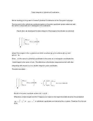
Recall when we developed the triple integral in Rectangular Coordinates we obtained:
where R is a region in the x-y plane over which a surface g(x,y) or surfaces g1(x,y) and
g2(x,y) lie.
Since z is the same in cylindrical coordinates is the same as in rectangular coordinates the
triple integral is the same in form. The difference is the double integral we are left with after
integrating with respect to z is a double integral in polar coordinates.
Therefore we obtain :
 h ( ) g
  2  2( x  y)
=    f ( r  z)  r dz dr d 
  
 h1(  ) g1( x  y
Recall in the polar coordinate system dA = r dr dθ .
What does a triple integral look like? Suppose our region is the region bounded above by the parabaloid
2 2 2
z 1x y or z 1r in cylindrical coordinates and below by the x-y plane. Therefore R is the unit
circle

2. 2
We integrate z from z = 0 to z 1r then r from 0 to 1 and θ from 0 to 2π .
See Animation Triple Integral in Cylindrical Coordinates.
2
2  1 1 r
  
Therefore we have    f ( r  z)  r dz dr d
  
0 0 0
Example 1
For the parabaloid above suppose f (r  z) r  1 the density increases radially as we move from the origin.
2
2  1 1 r
2
2  1 1 r
2
2  1 1 r


 
  f ( r  z)  r d r d  d z


 
  ( r  1)  r d z d r d 


 
   r 2  r  dz dr d
        
0 0 0 0 0 0 0 0 0
2
2  1 1 r 2  2 
r  r 
1 1
       2
  
2
 r dz dr d   2
 r  z 1  r
2
dr d 
3 4
 r  r  r  r dr d
      
0 0 0 0 0
  0
 
0 0
2 
2   2 

1
 2   r 3 r 4 r 5 r 2  23 23 23 

3 4
 r  r  r  r dr d        1 d  d   2 
  3 4 5 2  60 60 30
0 0  0  0
 0
0

3. Example 2
2
Find the volume of the solid bounded above by the parabaloid z 1  r and below by the parabaloid
2
z r
Recall V= ∭ dv
To set this up we find the curve of intersection and project this into the x-y plane to obtain R

4. 2 2
To find the curve of intersection we simply set z 1r equal to z r
2 2 1
r 1r from which we obtain r
2
1
2 
  2
2  1 r
 
Therefore we have V    r dz dr d
   2
0 0 r
1 1 1
2  2  2 
  2    
2  1 r   2   2
  2 3
   r dz dr d   r  z 1  r dr d   r  2 r d r d 
   2    
0 0 r 2 0 0
  r
 
0 0
1
2  2 
   2 
  2
  r 2 r 4 1  1 
 
3
r  2 r d r d      d  d
  2 2 2  8 4
0 0  
 0
0

0
Example 3
Suppose f(r,θ ,z) = z in the region which is in the cone z = r between the planes z = 1 and z = 4. Calculate it's
mass.

5. To set up the integral let's consider the cross-section corresponding to x = 0 .
We see that we're going to have to use 2 integrals . The solid gray region z varies from z = 1 to z =4
over a circle of radius 1. ( really we have a cylinder)
In the other region z varies from z = r to z = 4 over the annular region between r = 1 and r = 4
See the diagram below

6. 2  1 4 2  4 4
     
M    z r dz dr d     z r dz dr d
     
0 0 1 0 1 r
  255 
These are simple enough integrals so I'll leave it for you to verify M 15  225 .
2 4 4
Be Careful . Sometimes a person is tempted to simply use the geometric formula for a cylinder for the first integral. If
the density were constant we could do this. However the density here is a function of z so we have to use an integral.
Finally I'd like to give a geometric interpretation to the volume element rdzdrdθ .
Recall In Rectangular Coordinates we used the lines x = constant y = constant z =constant to divide
a region into cubes dxdydz.
In Cylindrical coordinates we use r = constant θ = constant z = constant to obtain :