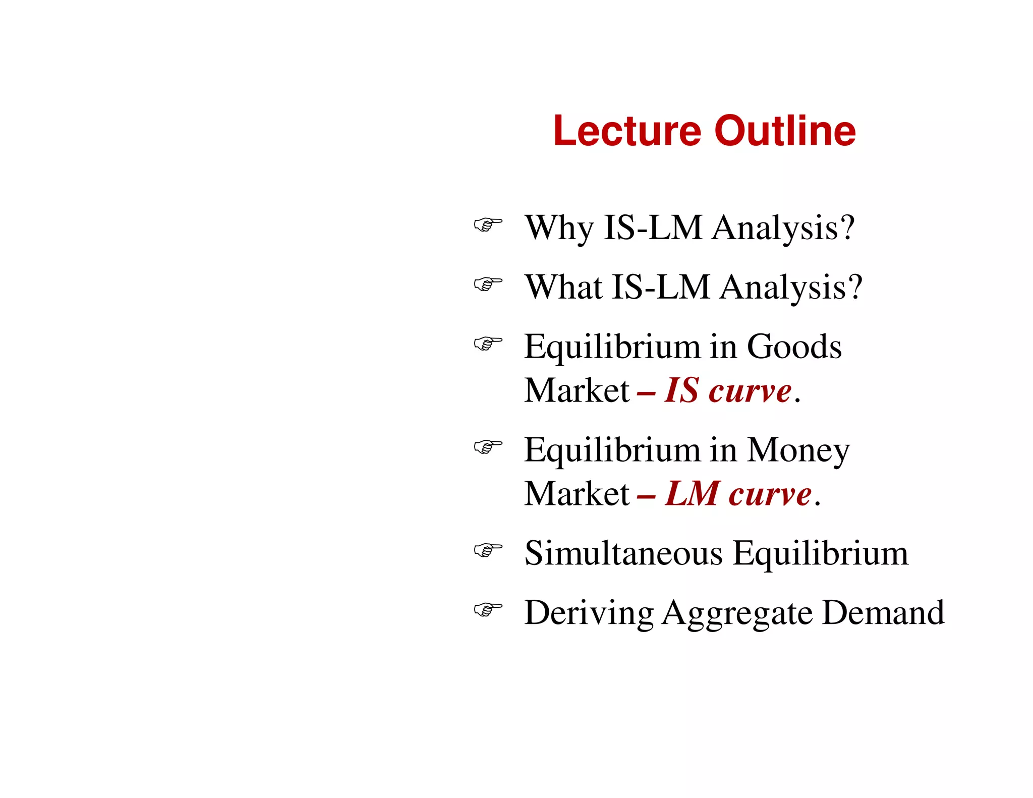
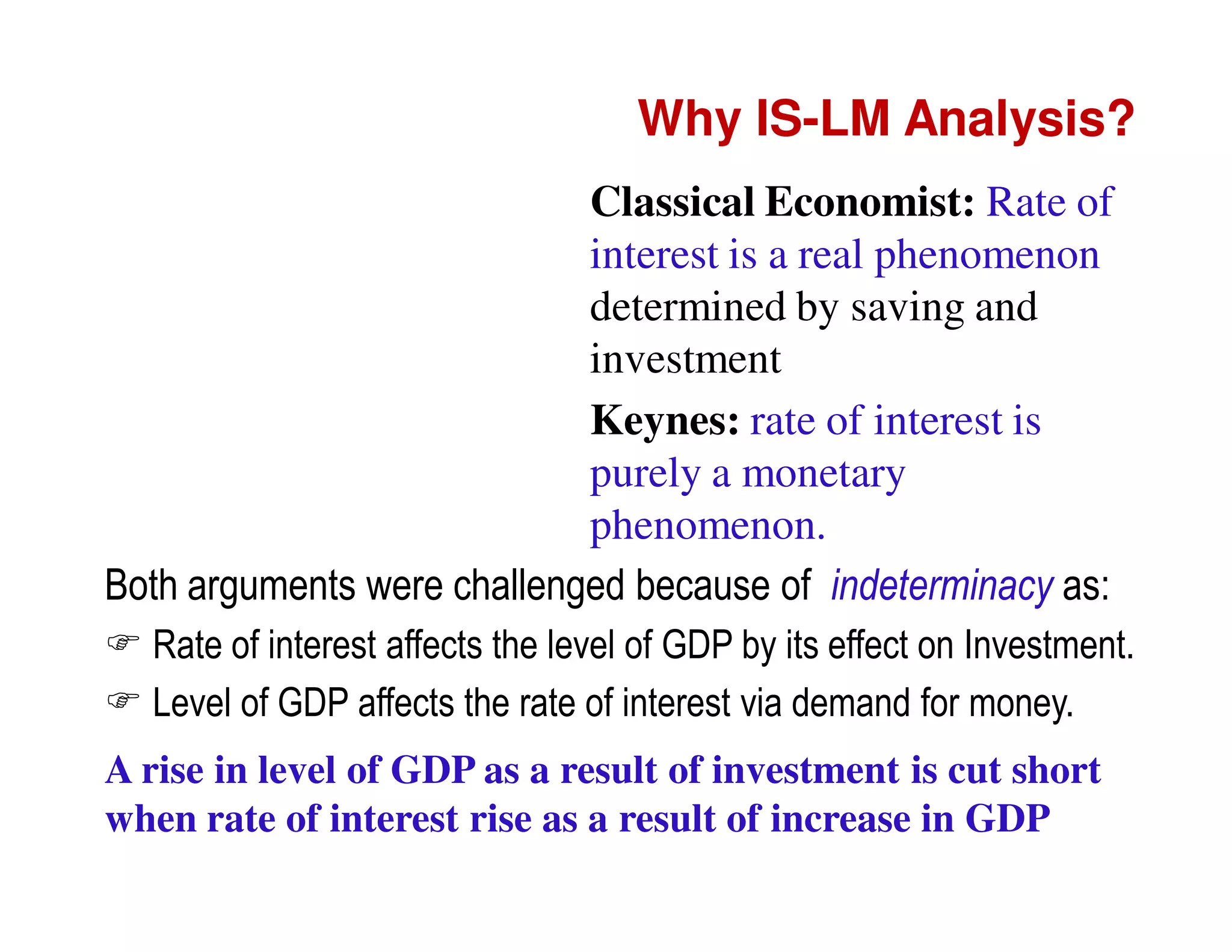
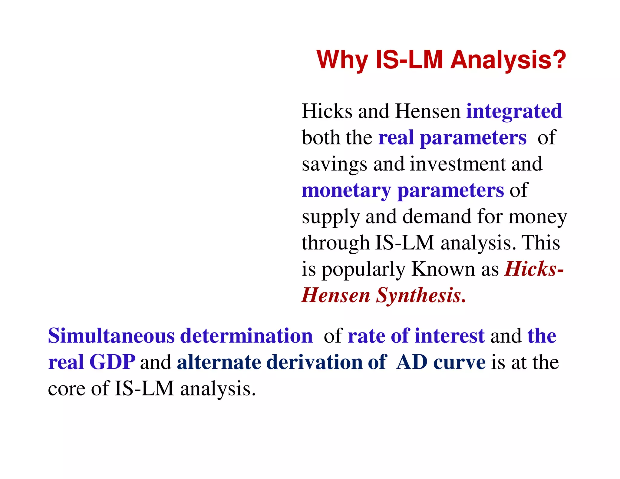
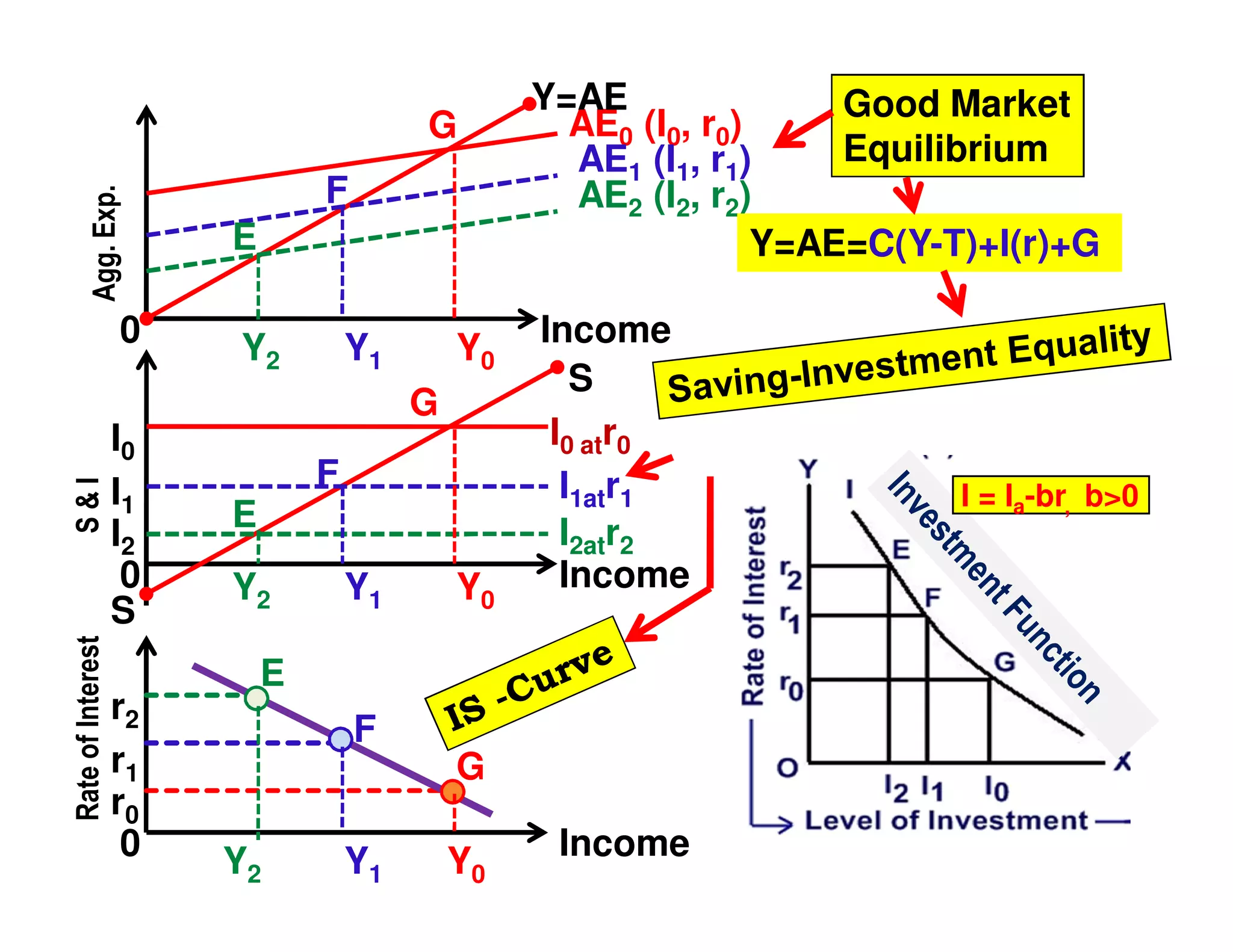
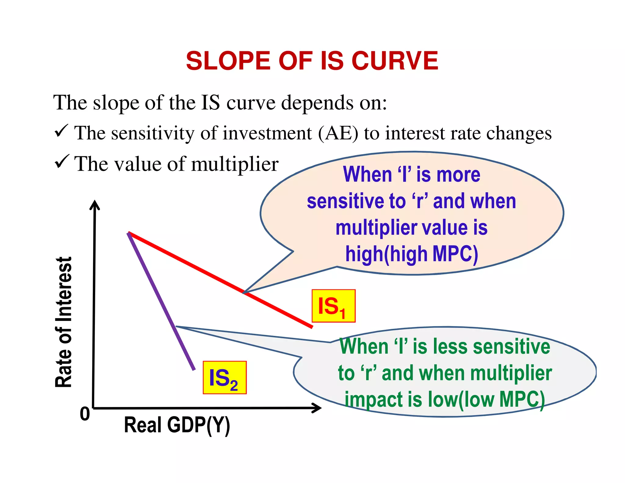
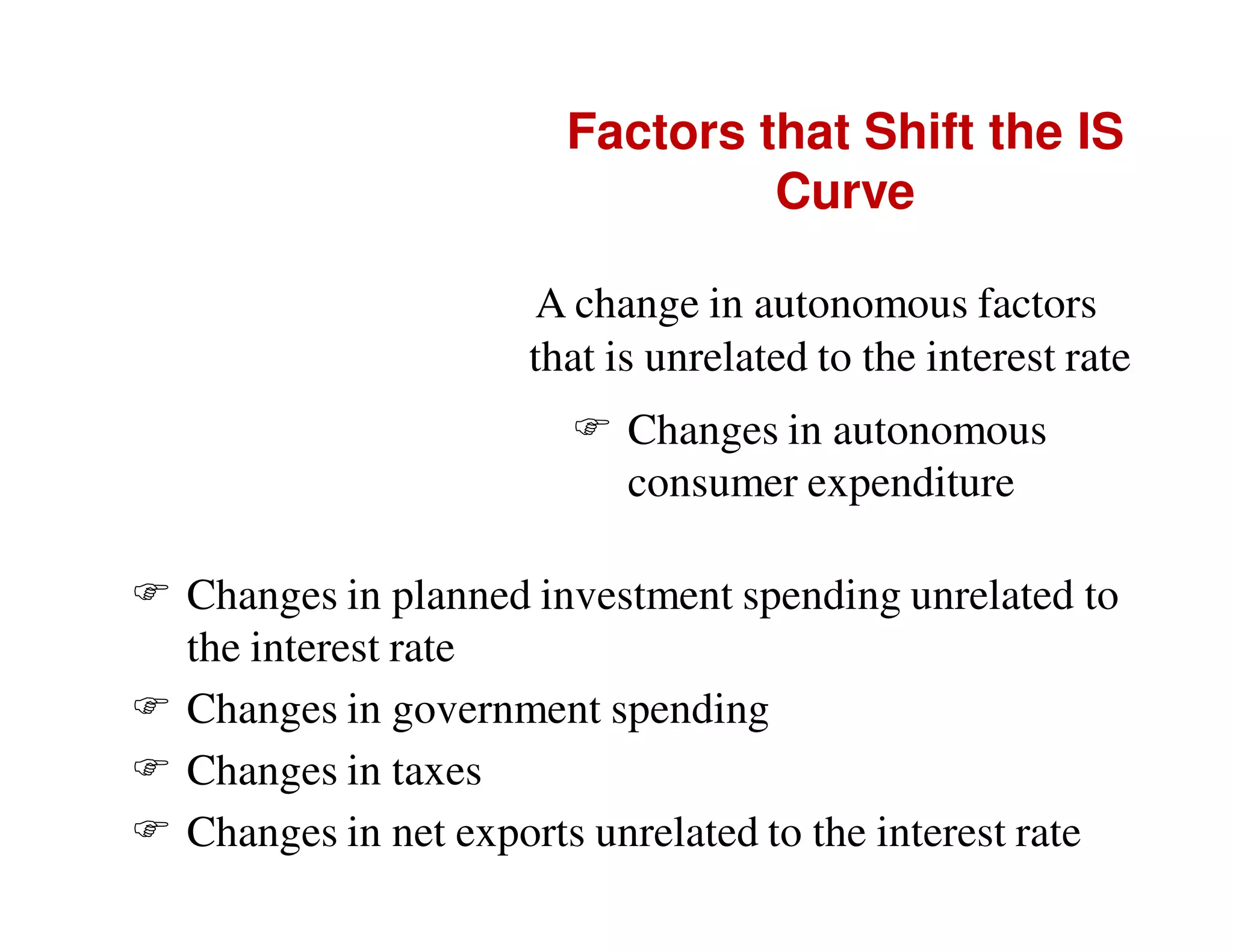
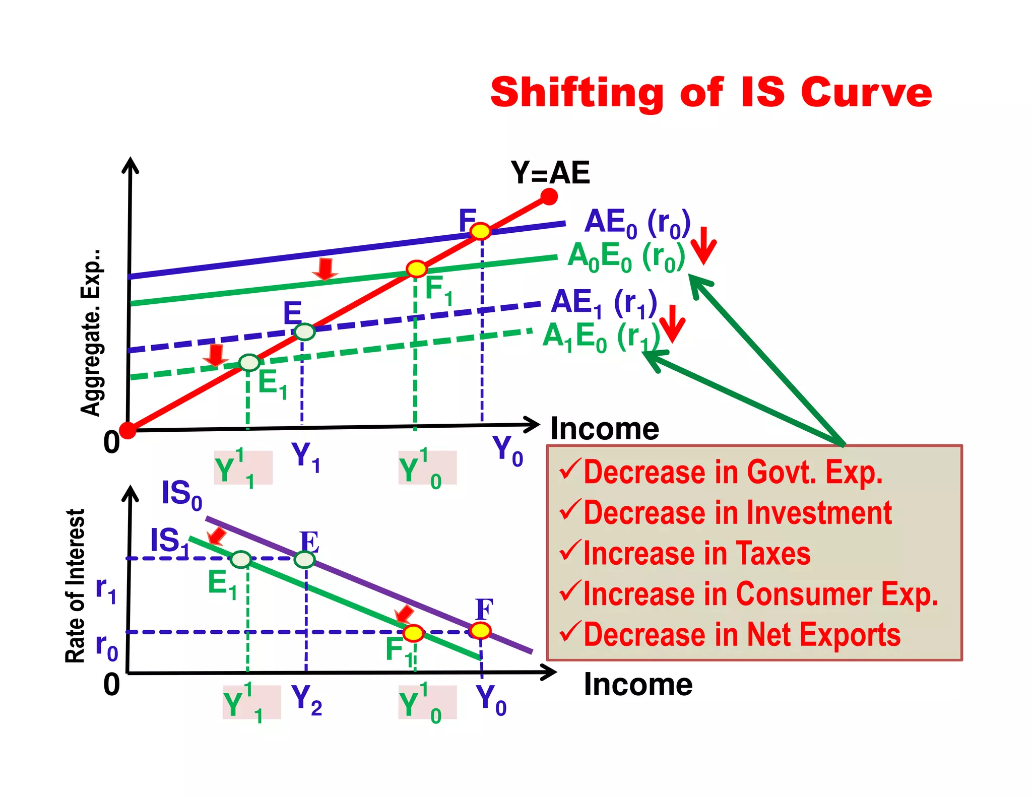
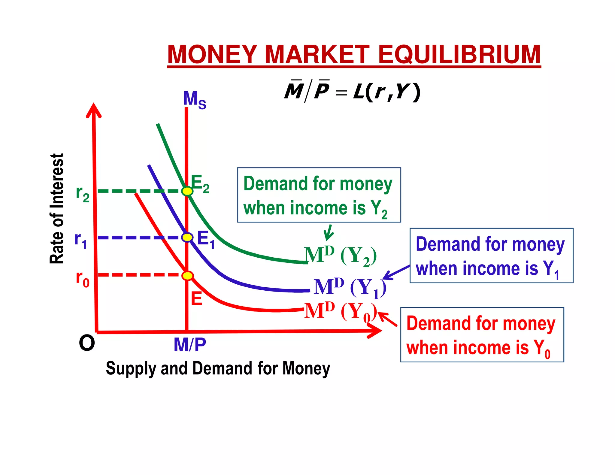
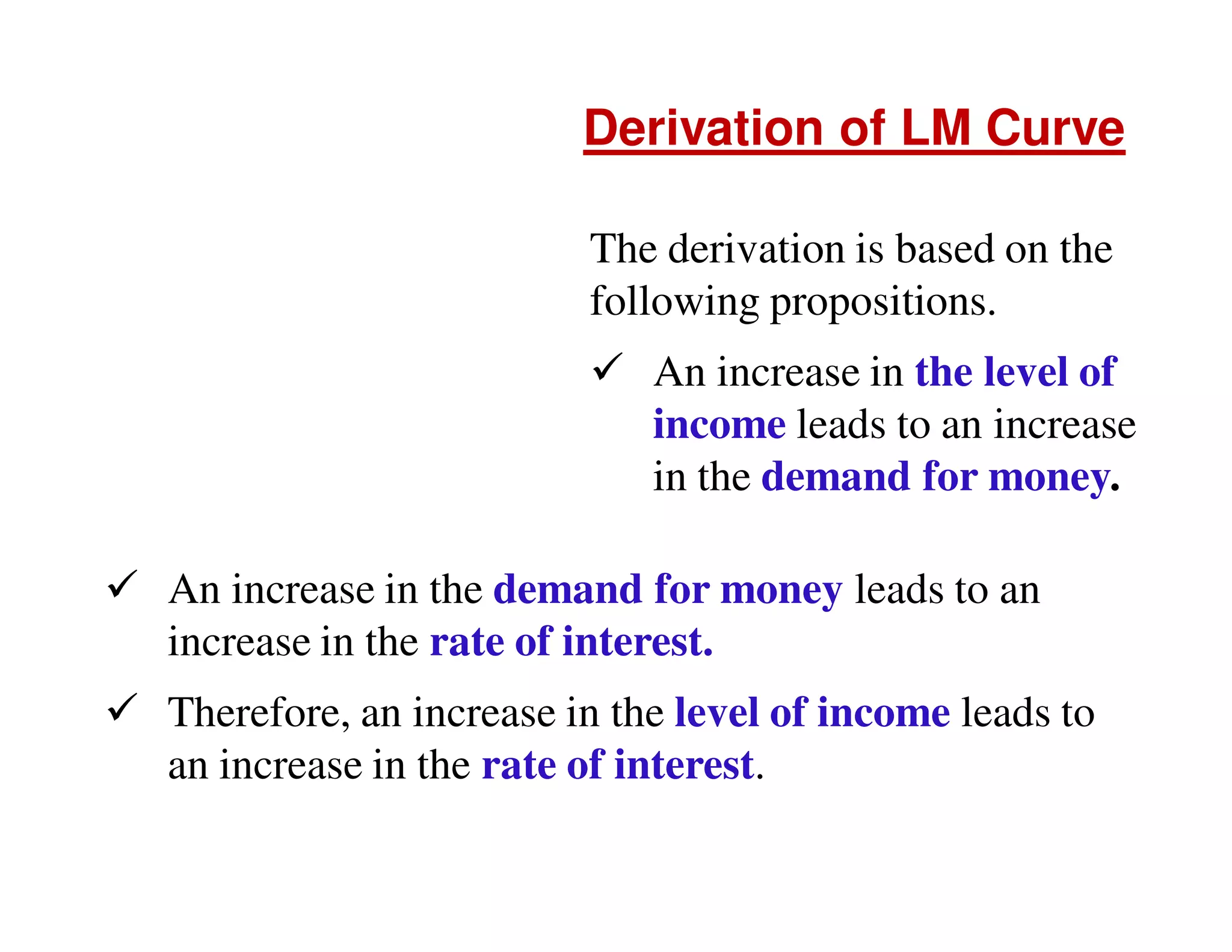
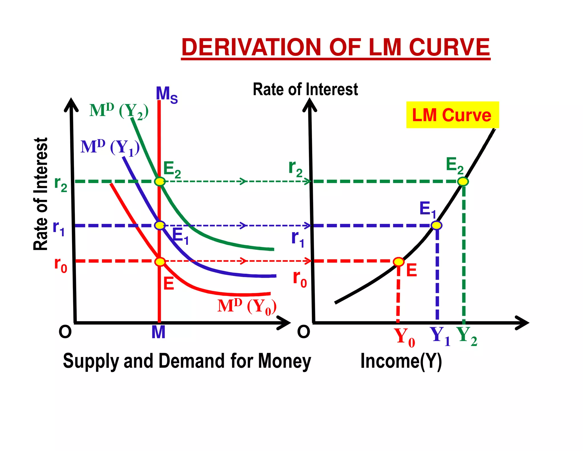
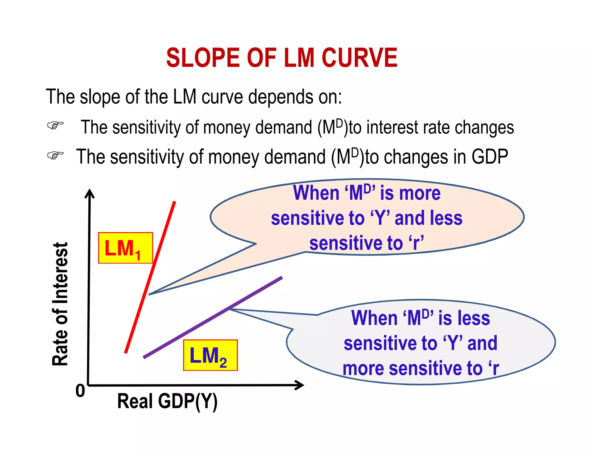
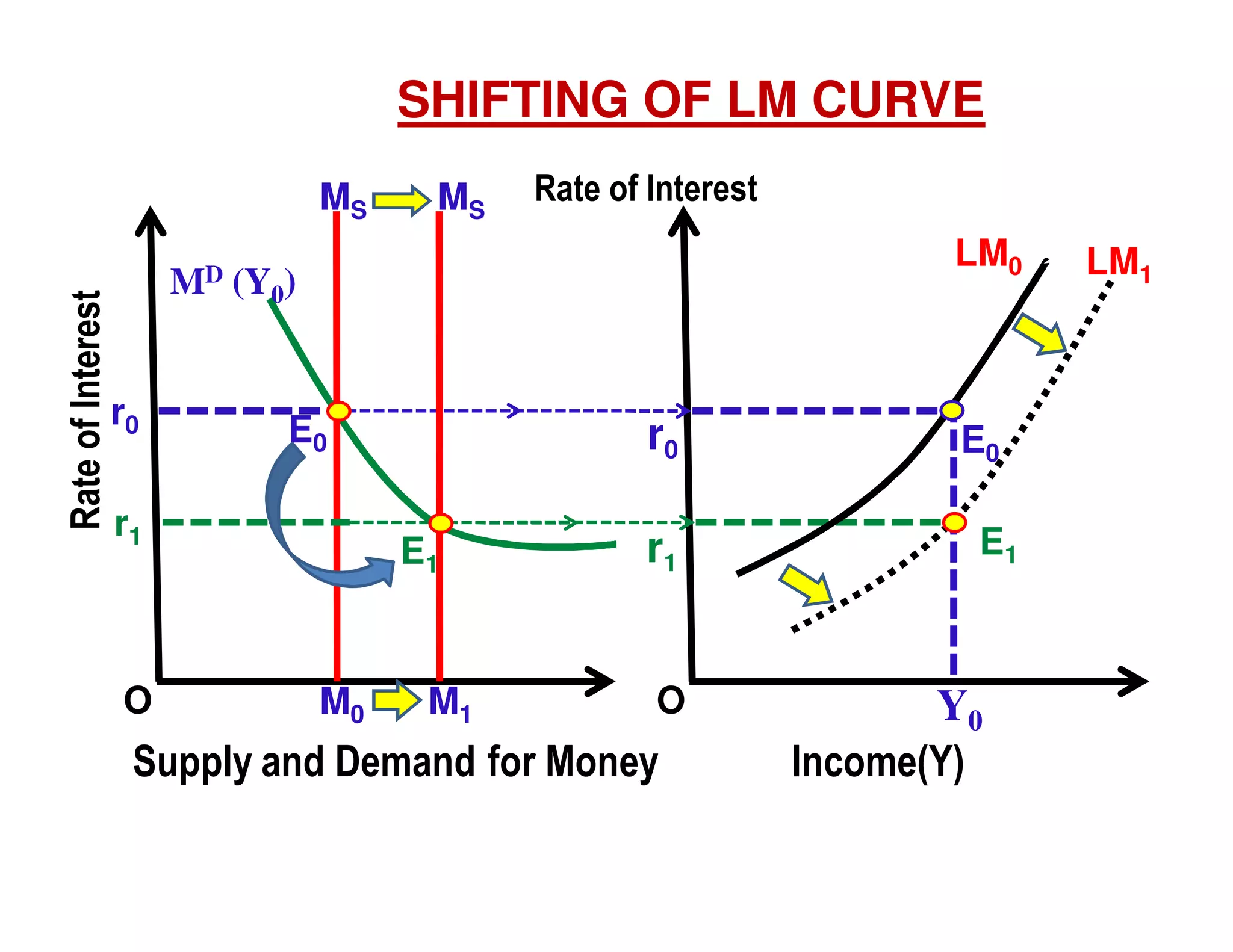
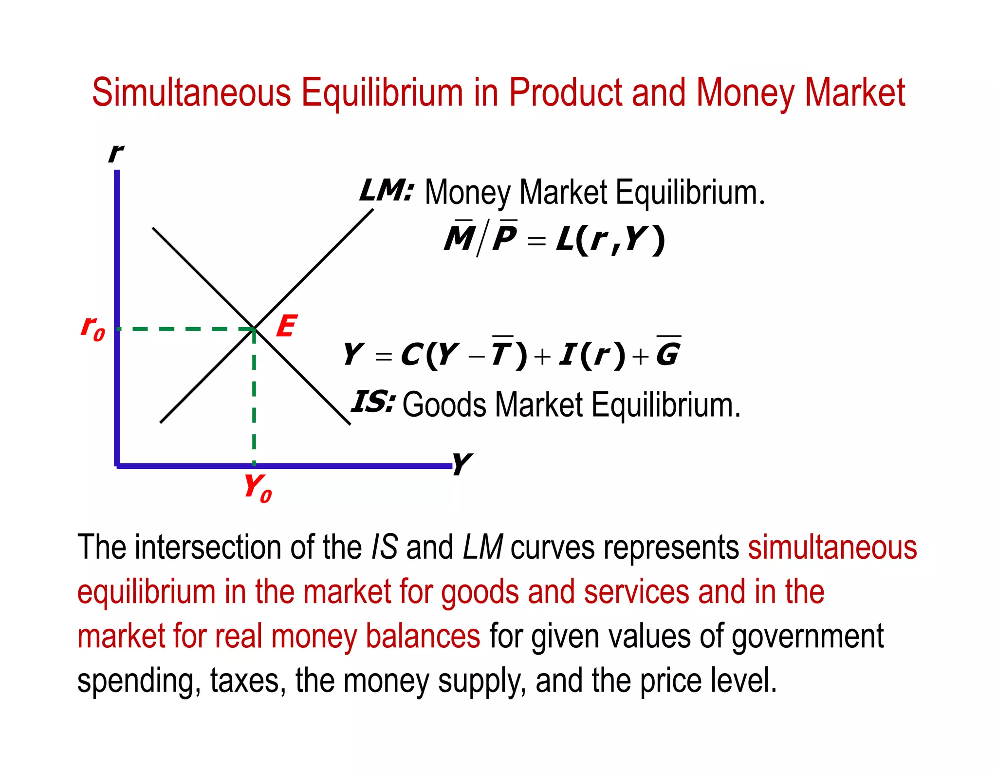
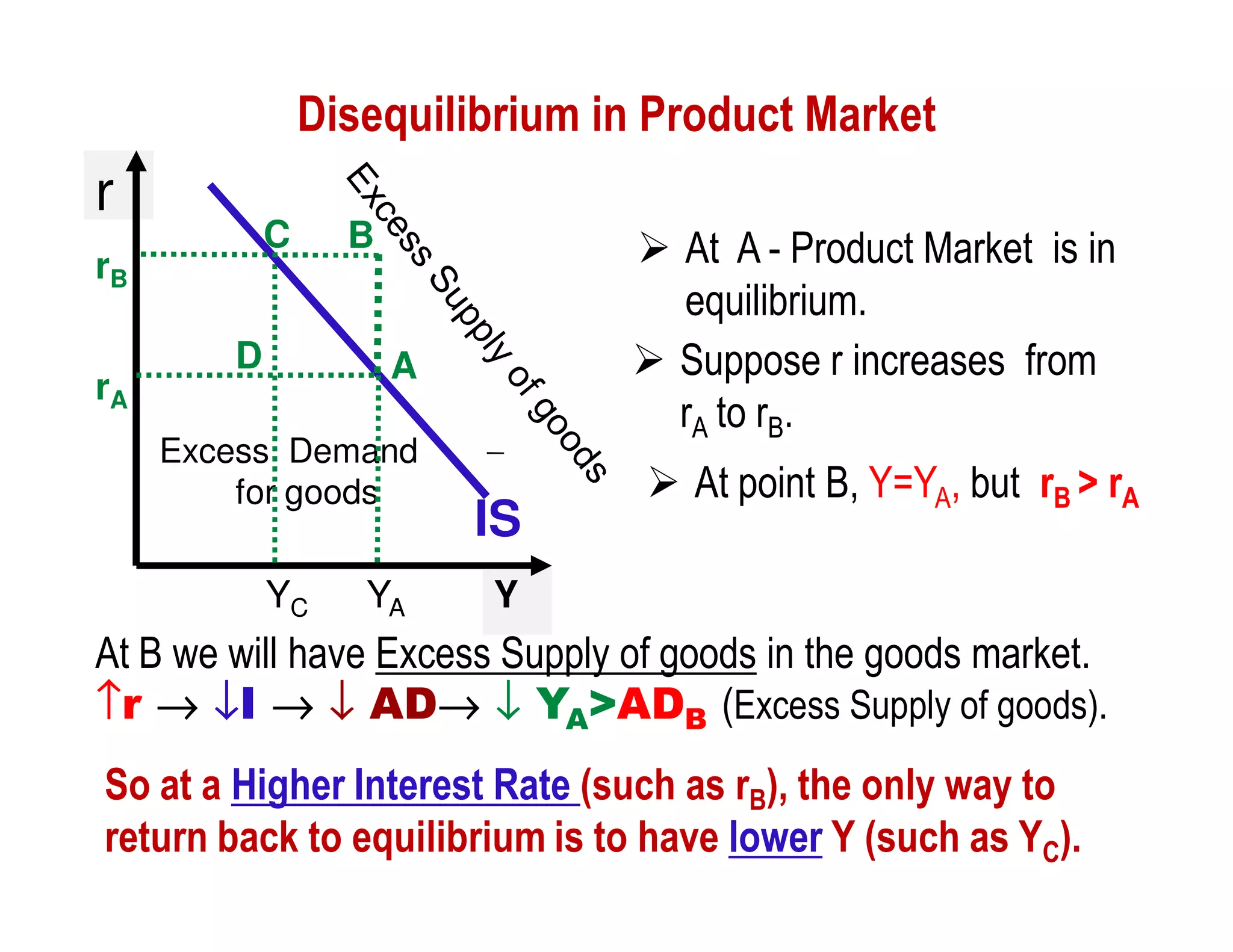
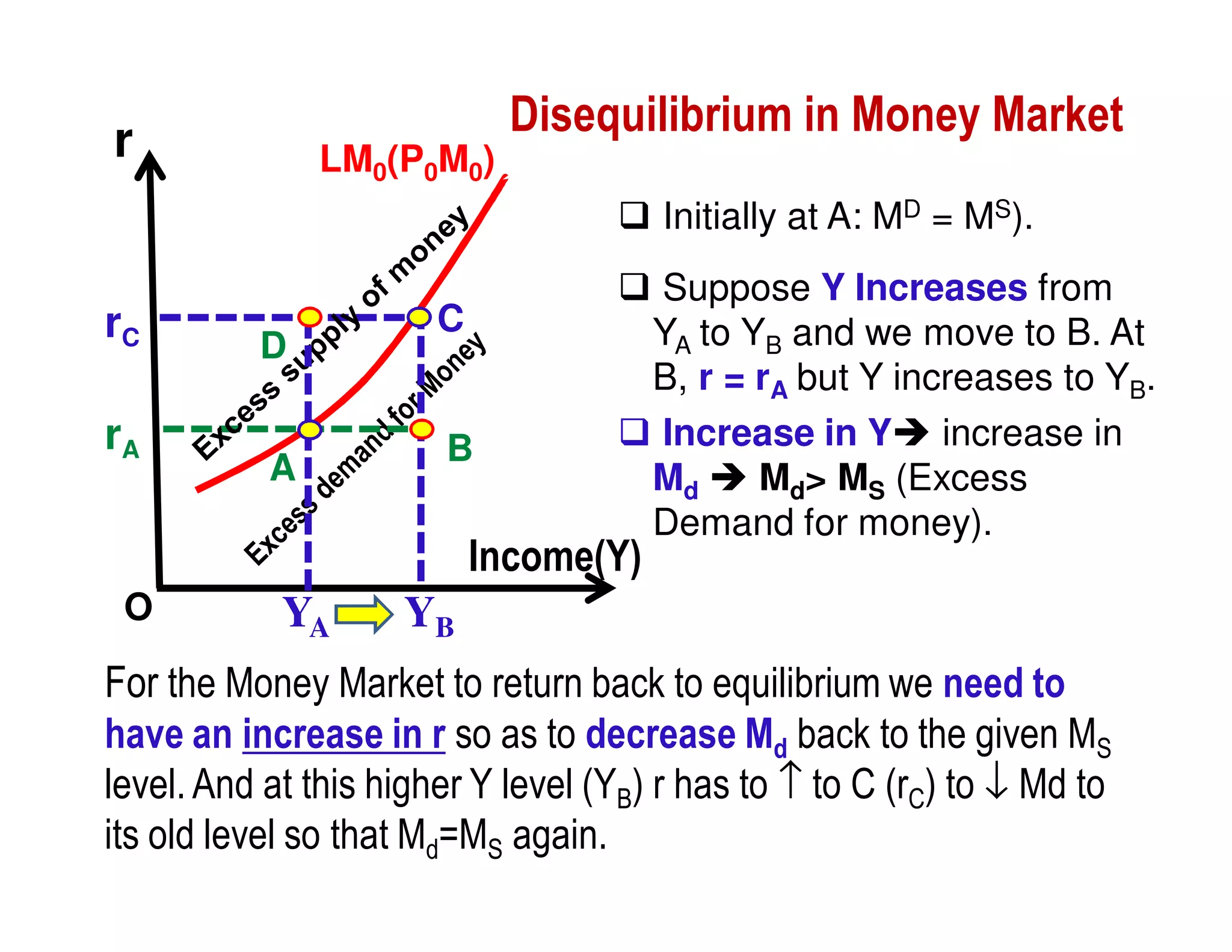
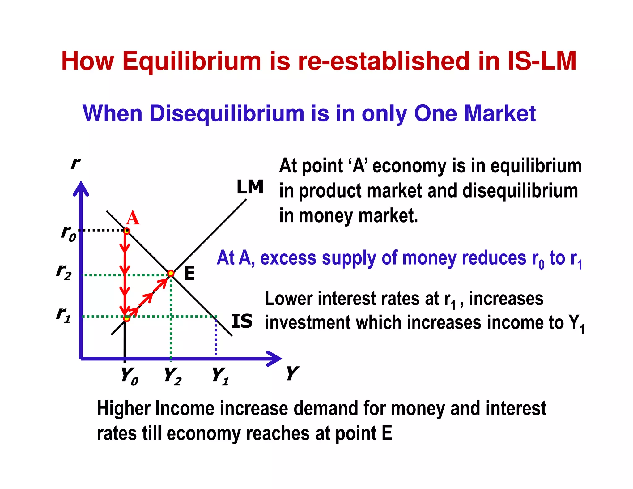
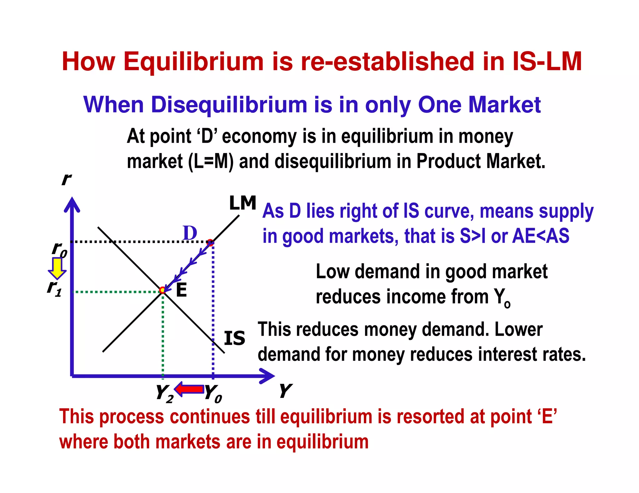
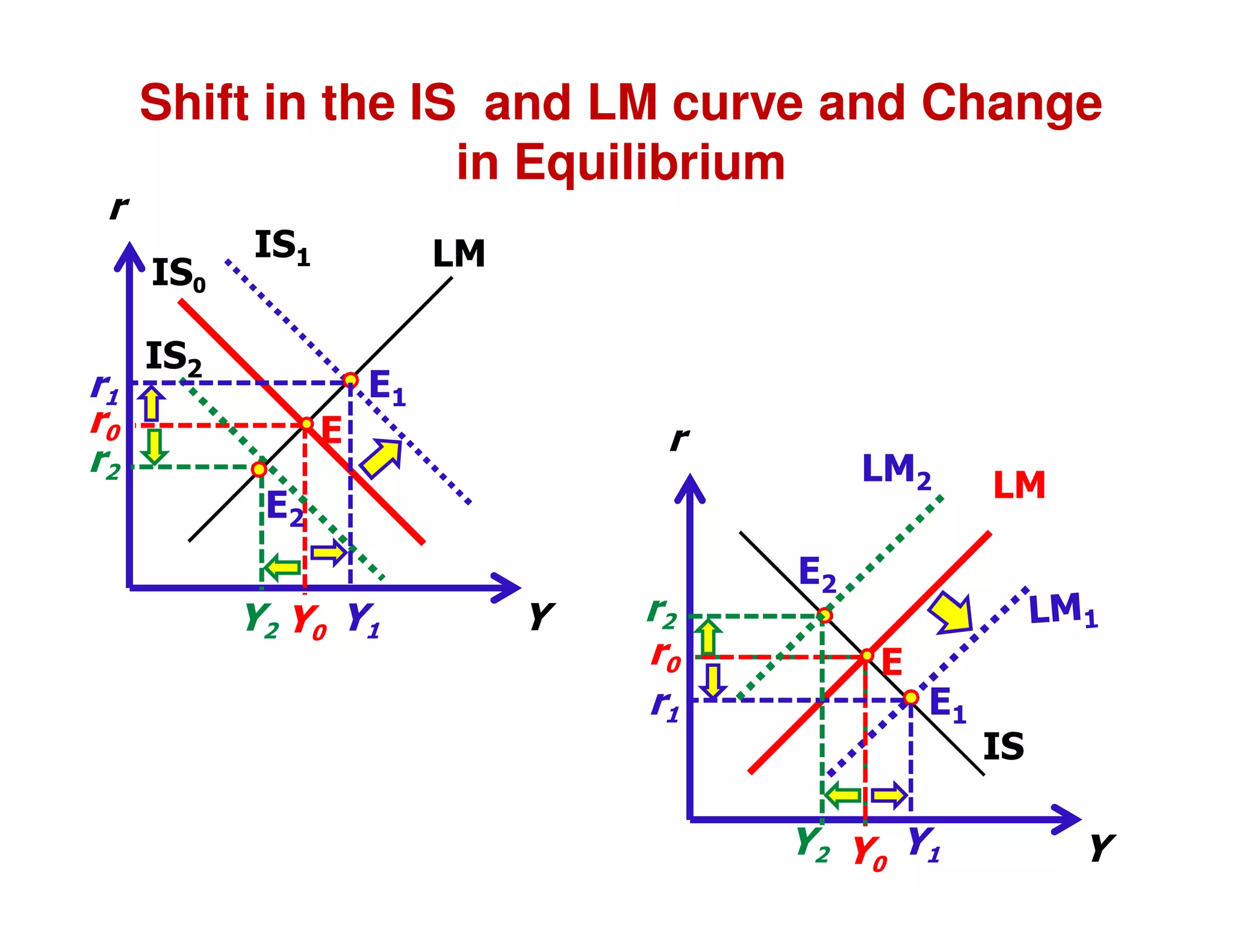
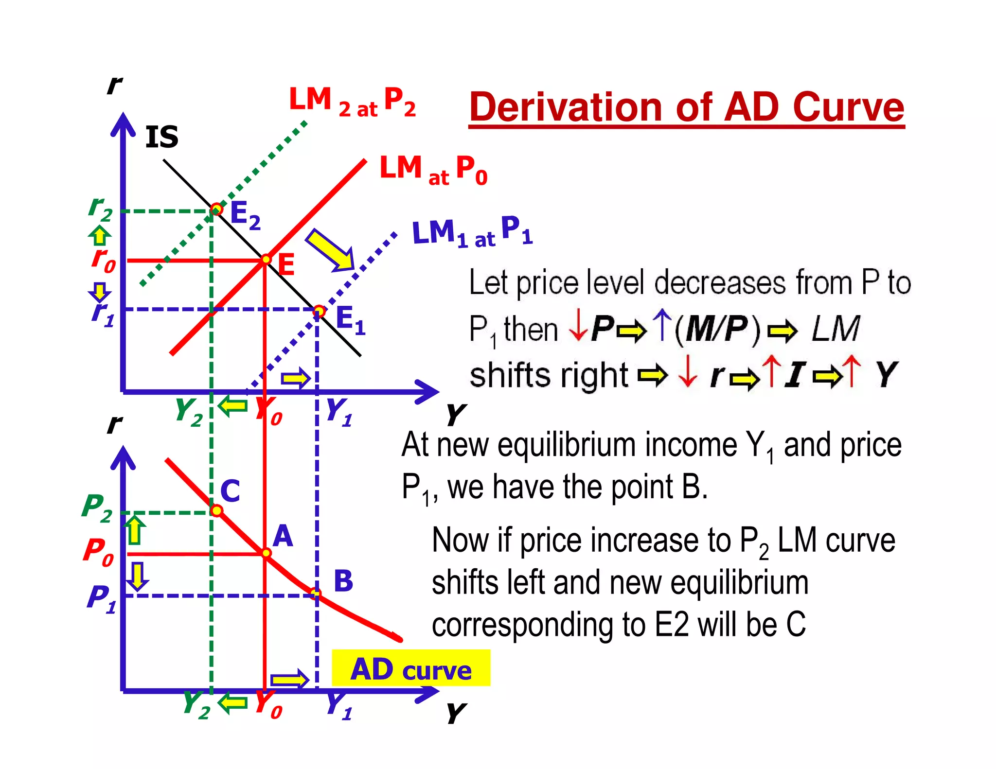
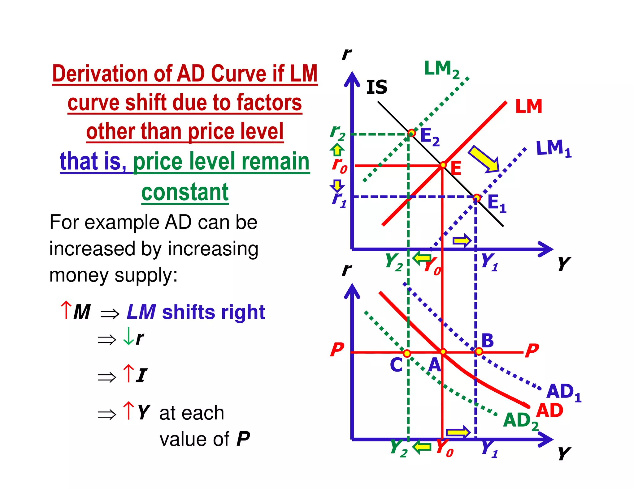
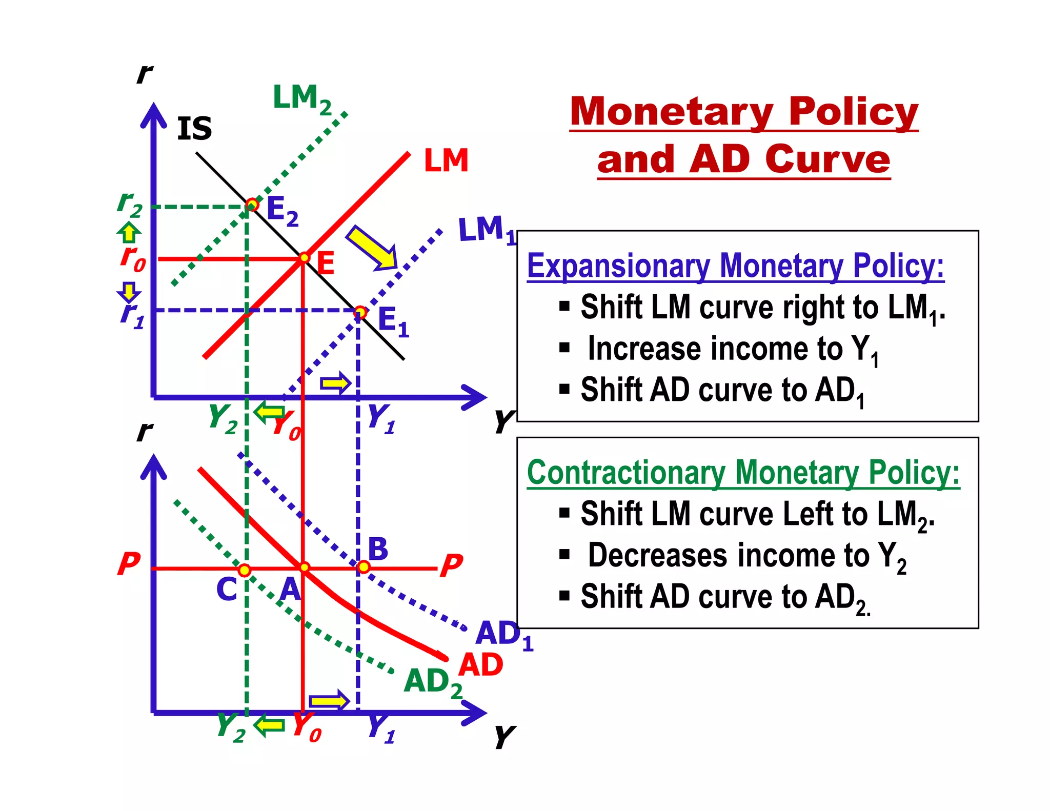
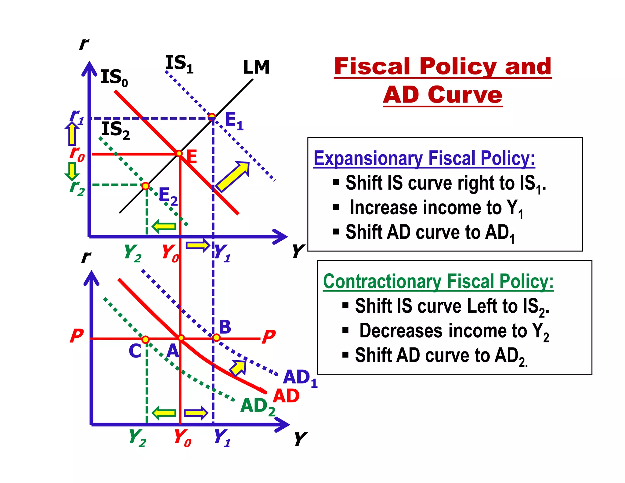
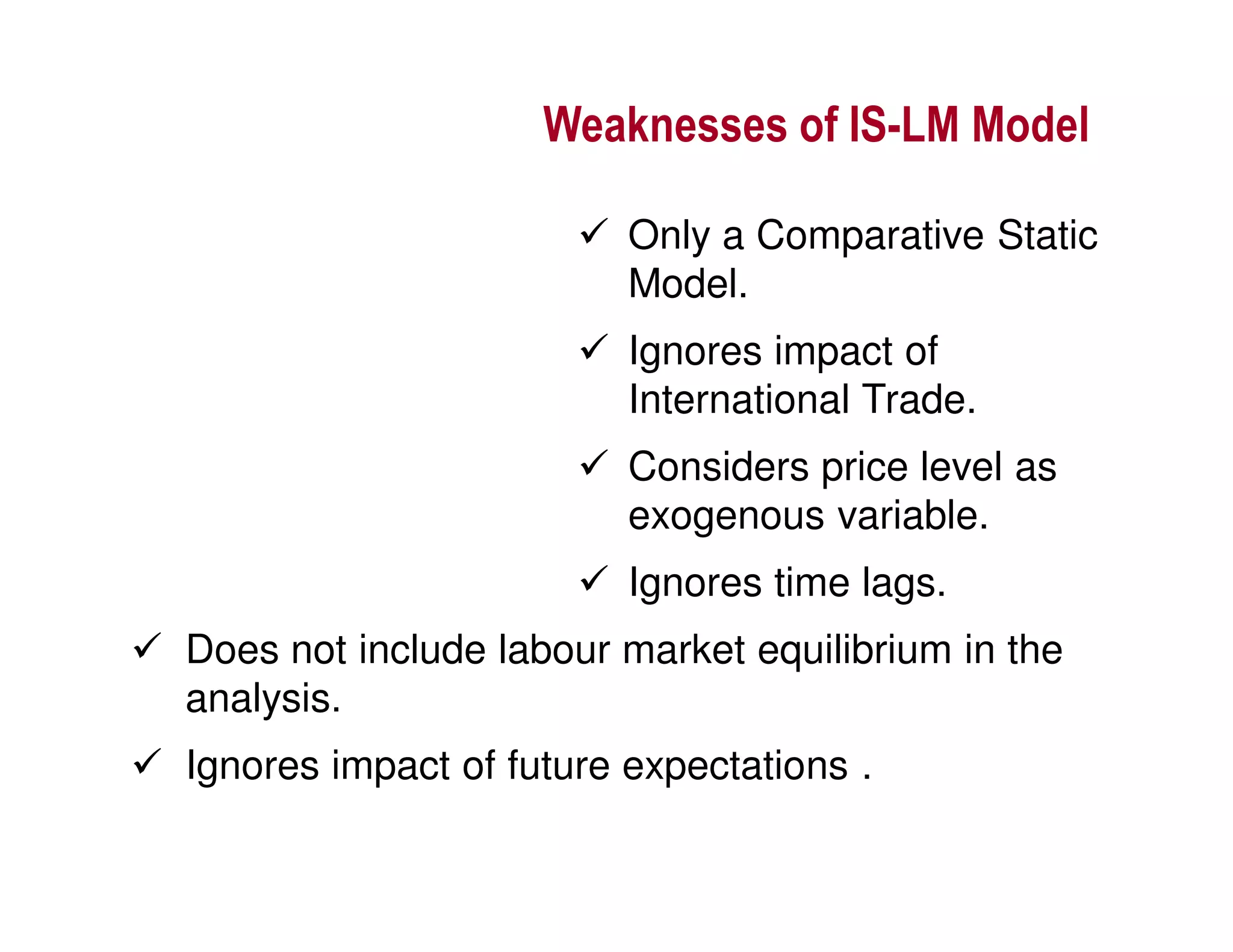
This document provides an outline and explanation of IS-LM analysis and how it can be used to derive the aggregate demand curve. It begins by explaining why IS-LM analysis was developed as a synthesis of classical and Keynesian thought. It then defines the IS curve as representing goods market equilibrium and the LM curve as representing money market equilibrium. It shows how the intersection of the IS and LM curves determines the equilibrium interest rate and level of output. It further explains how shifts in the IS and LM curves affect this equilibrium and can be used to trace the aggregate demand curve. Fiscal and monetary policy shifts are also discussed through their impacts on the IS and LM curves.

1. IS-LM ANALYSIS
AND
AGGREGATE
DEMAND
DR. LAXMI NARAYAN
ASSISTANT PROFESSOR OF ECONOMICS
GOVT. COLLEGE FOR WOMEN, BHODIA KHERA

2. Lecture Outline
Why IS-LM Analysis?
What IS-LM Analysis?
Equilibrium in Goods
Market – IS curve.
Equilibrium in Money
Market – LM curve.
Simultaneous Equilibrium
Deriving Aggregate Demand

3. Why IS-LM Analysis?
Classical Economist: Rate of
interest is a real phenomenon
determined by saving and
investment
Keynes: rate of interest is
purely a monetary
phenomenon.
Both arguments were challenged because of indeterminacy as:
Rate of interest affects the level of GDP by its effect on Investment.
Level of GDP affects the rate of interest via demand for money.
A rise in level of GDP as a result of investment is cut short
when rate of interest rise as a result of increase in GDP

4. Why IS-LM Analysis?
Hicks and Hensen integrated
both the real parameters of
savings and investment and
monetary parameters of
supply and demand for money
through IS-LM analysis. This
is popularly Known as HicksHensen Synthesis.
Simultaneous determination of rate of interest and the
real GDP and alternate derivation of AD curve is at the
core of IS-LM analysis.

5. What is IS-LM Analysis?
The term IS refers to the
equality between Investment(I)
& saving(S) the corresponding
equilibrium in the Goods
Market.
The term LM refers to the equality between demand for
money (L)& Supply of money (M) and the corresponding
equilibrium in Money Market.

6. IS Curve and Product
Market Equilibrium?
IS curve is the locus of different
combinations of Interest Rate(r)
and Level of GDP (Y) that are
consistent with equality between
saving and Investment or
Aggregate Output and Aggregate
Expenditure.
The IS curve represents all combinations of income (Y) and
the real interest rate (r) such that the market for goods and
services is in equilibrium. That is, every point on the IS
curve is an income/real interest rate pair (Y, r) such that the
demand for goods is equal to the supply of goods.

7. Derivation of IS Curve
IS curve is derived from using three
relationships:
Investment Demand Function.
Changes in the Aggregate
Expenditure as a result of change
in investment when r changes.
Relationship between different level of ‘r’ and ‘GDP’ and the
equality between ‘S’ & ‘I’ that is IS curve.

8. Derivation of IS Curve
The derivation is based on the
following propositions.
An increase in rate of
Interest leads to a decrease
in the level of Investment.
An decrease in the level of investment leads to a
decrease in the level of income.
Therefore, an increase in the rate of interest leads to a
decrease in the rate of interest.

9. Agg. Exp.
G
Rate of Interest
S&I
0
I0
I1
I2
0
S
r2
r1
r0
0
F
E
Y2
Y1
Y0
G
F
E
Y2
Y1
Y0
Y=AE
Good Market
AE0 (I0, r0)
Equilibrium
AE1 (I1, r1)
AE2 (I2, r2)
Y=AE=C(Y-T)+I(r)+G
Income
S
I0 atr0
I1atr1
I2atr2
Income
E
F
G
Y2
Y1
Y0
Income
I = Ia-br, b>0

10. SLOPE OF IS CURVE
The slope of the IS curve depends on:
The sensitivity of investment (AE) to interest rate changes
Rate of Interest
The value of multiplier
When ‘I’ is more
sensitive to ‘r’ and when
multiplier value is
high(high MPC)
IS1
IS2
0
Real GDP(Y)
When ‘I’ is less sensitive
to ‘r’ and when multiplier
impact is low(low MPC)

11. Factors that Shift the IS
Curve
A change in autonomous factors
that is unrelated to the interest rate
Changes in autonomous
consumer expenditure
Changes in planned investment spending unrelated to
the interest rate
Changes in government spending
Changes in taxes
Changes in net exports unrelated to the interest rate

12. Shifting of IS Curve
Y=AE
Aggregate. Exp..
F
E1
Rate of Interest
IS0
1
Y1
IS1
r0
0
F1
E
0
r1
AE0 (r0)
A0E0 (r0)
AE1 (r1)
A1E0 (r1)
Y1
1
Y0
Y0
E
E1
F
F1
1
Y1
Y2
1
Y0
Y0
Income
Decrease in Govt. Exp.
Decrease in Investment
Increase in Taxes
Increase in Consumer Exp.
Decrease in Net Exports
Income

13. LM Curve and Money
Market Equilibrium?
The LM curve shows all the
combinations of interest rates i
and outputs Y for which the
money market is in equilibrium.
"L" denotes Liquidity and "M"
denotes money,
The LM curve, is a graph of combinations of real income, Y,
and the real interest rate, r, such that the money market is in
equilibrium (i.e. real money supply = real money demand).

14. DEMAND FOR MONEY
Transaction Demand for Money(Mt)
Y
K
Mt = K(y) : 1>K>0
K = Proportion of income kept
Y1
Y0
is cash for transaction purpose
Mt
O
M0 M1
r
Speculative Demand for Money(Ms)
Ms = L(r) : L`<0
r1
r2
Liquidity Trap
r0
O M1 M2
Ms

15. Total Demand for money
Rate of Interest
Supply of Money
O
MS
Rate of Interest
YD
r1
O
M
Supply of Money
MD = Mt + Ms
or
MD = K(y) + L(r)
MD (YD)
M0
M1
Demand for Money

16. MONEY MARKET EQUILIBRIUM
Rate of Interest
MS
r2
r1
E2
E1
r0
E
O
M P = L (r ,Y )
Demand for money
when income is Y2
MD
(Y2)
MD (Y1)
MD (Y0)
M/P
Supply and Demand for Money
Demand for money
when income is Y1
Demand for money
when income is Y0

17. Derivation of LM Curve
The derivation is based on the
following propositions.
An increase in the level of
income leads to an increase
in the demand for money.
An increase in the demand for money leads to an
increase in the rate of interest.
Therefore, an increase in the level of income leads to
an increase in the rate of interest.

18. DERIVATION OF LM CURVE
Rate of Interest
MD (Y2)
MS
Rate of Interest
LM Curve
MD (Y1)
r2
E2
r2
E2
E1
r1
E1
r1
r0
r0
E
E
MD (Y0)
O
M
O
Supply and Demand for Money
Y0 Y1 Y2
Income(Y)

19. SLOPE OF LM CURVE
The slope of the LM curve depends on:
The sensitivity of money demand (MD)to interest rate changes
The sensitivity of money demand (MD)to changes in GDP
When ‘MD’ is more
sensitive to ‘Y’ and less
sensitive to ‘r’
Rate of Interest
LM1
LM2
0
Real GDP(Y)
When ‘MD’ is less
sensitive to ‘Y’ and
more sensitive to ‘r

20. SHIFTING OF LM CURVE
Rate of Interest
MS
MD
r0
Rate of Interest
LM0
(Y0)
E0
r1
O
MS
r0
E1
M0
M1
r1
O
Supply and Demand for Money
E0
E1
Y0
Income(Y)
LM1

21. Simultaneous Equilibrium in Product and Money Market
r
LM: Money Market Equilibrium.
M P = L (r ,Y )
r0
E
Y0
Y = C ( − T ) + I (r ) + G
Y
IS: Goods Market Equilibrium.
Y
The intersection of the IS and LM curves represents simultaneous
equilibrium in the market for goods and services and in the
market for real money balances for given values of government
spending, taxes, the money supply, and the price level.

22. Disequilibrium in Product Market
r
C
rB
rA
D
B
At A - Product Market is in
equilibrium.
Suppose r increases from
rA to rB.
A
Excess Demand
for goods
YC
YA
IS
At point B, Y=YA, but rB > rA
Y
At B we will have Excess Supply of goods in the goods market.
↑r → ↓I → ↓ AD→ ↓ YA>ADB (Excess Supply of goods).
→
So at a Higher Interest Rate (such as rB), the only way to
return back to equilibrium is to have lower Y (such as YC).

23. Disequilibrium in Money Market
r
LM0(P0M0)
Initially at A: MD = MS).
rC
rA
D
A
C
B
Income(Y)
O
YA
Suppose Y Increases from
YA to YB and we move to B. At
B, r = rA but Y increases to YB.
Increase in Y increase in
Md
Md> MS (Excess
Demand for money).
YB
For the Money Market to return back to equilibrium we need to
have an increase in r so as to decrease Md back to the given MS
level. And at this higher Y level (YB) r has to ↑ to C (rC) to ↓ Md to
its old level so that Md=MS again.

24. Disequilibrium in IS-LM
We can conclude:
If disequilibrium is at the
right of IS curve indicating
Excess Supply in Goods
market, only way to restore
equilibrium is to decrease Y.
same way for point on the
left, increase Y.
If disequilibrium is at the right of LM curve indicating
Excess Demand for Money in money market, only way to
restore equilibrium is to increase rate of interest(r).
Same way for points on the left of the LM, decrease ‘r’

25. Disequilibrium in IS-LM
r
Any point other than point E
is point of disequilibrium.
Point A&B: I=S but L≠ M
Point M&N: L=M but I≠ S
LM
r0
B
T
N
M
L
E
V
Point K: L>M & S<I
KA
Y0
IS
Y
Point V: L>M & S>I
Point L: L<M & S<I
Point K: L<M & S<I

26. How Equilibrium is re-established in IS-LM
When Disequilibrium is in only One Market
r
r0
At point ‘A’ economy is in equilibrium
LM in product market and disequilibrium
in money market.
A
r2
E
At A, excess supply of money reduces r0 to r1
Lower interest rates at r1 , increases
IS investment which increases income to Y1
r1
Y0
Y2
Y1
Y
Higher Income increase demand for money and interest
rates till economy reaches at point E

27. How Equilibrium is re-established in IS-LM
When Disequilibrium is in only One Market
r
At point ‘D’ economy is in equilibrium in money
market (L=M) and disequilibrium in Product Market.
LM As D lies right of IS curve, means supply
r0
r1
D
E
in good markets, that is S>I or AE<AS
Low demand in good market
reduces income from Yo
IS This reduces money demand. Lower
demand for money reduces interest rates.
Y
Y2 Y0
This process continues till equilibrium is resorted at point ‘E’
where both markets are in equilibrium

28. r
Shift in the IS and LM curve and Change
in Equilibrium
IS0
r1
r0
r2
IS1
LM
IS2
E1
E
r
LM2
E2
Y2 Y0 Y1
Y
r2
r0
r1
LM
E2
E
E1
IS
Y2 Y0 Y1
Y

29. r
LM 2 at P2
Derivation of AD Curve
IS
LM at P0
r2
E2
r0
E
r1
r
E1
Y0
Y2
Y1
C
P2
P0
P1
A
B
Y
At new equilibrium income Y1 and price
P1, we have the point B.
Now if price increase to P2 LM curve
shifts left and new equilibrium
corresponding to E2 will be C
AD curve
Y2
Y0
Y1
Y

30. r
LM2
Derivation of AD Curve if LM
IS
curve shift due to factors
r2
other than price level
that is, price level remain
constant
For example AD can be
increased by increasing
money supply:
↑M ⇒ LM shifts right
⇒ ↓r
⇒ ↑I
⇒ ↑Y at each
value of P
LM
E2
r0
E
r1
r
P
E1
Y2 Y0
Y1
B
C
A
Y
P
AD1
AD AD
2
Y2
Y0
Y1
Y

31. r
LM2
IS
Monetary Policy
and AD Curve
LM
r2
E2
r0
E
r1
r
P
E1
Y2 Y0
Y1
B
C
A
Y
Expansionary Monetary Policy:
Shift LM curve right to LM1.
Increase income to Y1
Shift AD curve to AD1
Contractionary Monetary Policy:
Shift LM curve Left to LM2.
Decreases income to Y2
Shift AD curve to AD2.
P
AD1
AD AD
2
Y2
Y0
Y1
Y

32. r
IS1
IS0
r1
E1
IS2
r0
E
r2
r
P
Fiscal Policy and
AD Curve
LM
E2
Y2 Y0
B
C
Y
Y1
A
Expansionary Fiscal Policy:
Shift IS curve right to IS1.
Increase income to Y1
Shift AD curve to AD1
P
AD1
AD AD
2
Y2
Y0
Y1
Y
Contractionary Fiscal Policy:
Shift IS curve Left to IS2.
Decreases income to Y2
Shift AD curve to AD2.

33. Weaknesses of IS-LM Model
Only a Comparative Static
Model.
Ignores impact of
International Trade.
Considers price level as
exogenous variable.
Ignores time lags.
Does not include labour market equilibrium in the
analysis.
Ignores impact of future expectations .

34. REFERENCES
Jain, T.R and Majhi, B.D.,
“Macroeconomics” V.K.
Publications.
Rana, K.C. and Verma,
K.N., “Macro Economic
Analysis” Vishaal
Publications.
Rana, A.S., “Advance Macro Economics-Theory and
Policy,” Kalyani Publishers.
Shapiro, E, “Macro Economic Analysis” Galgotia
Publications.

35. FAQs
Explain the determination of
GDP and rate of interest with
the help of IS-LM curve
Analysis.
Trace the derivation of IS and
LM curves.
Derive the aggregate demand curve through IS-LM curve
Model.
Explain the effect of Monetary and Fiscal policy through IS-LM
Model.