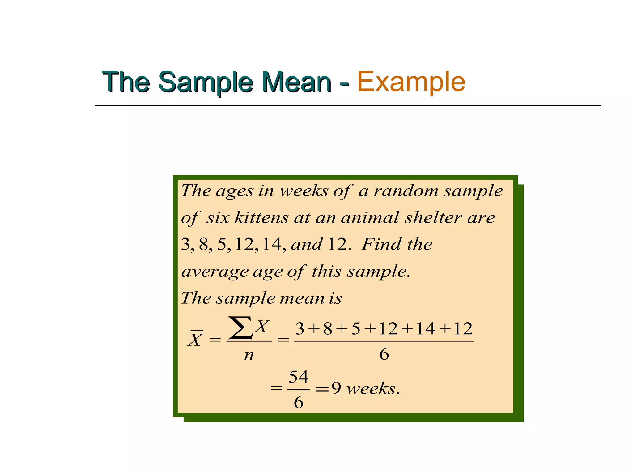
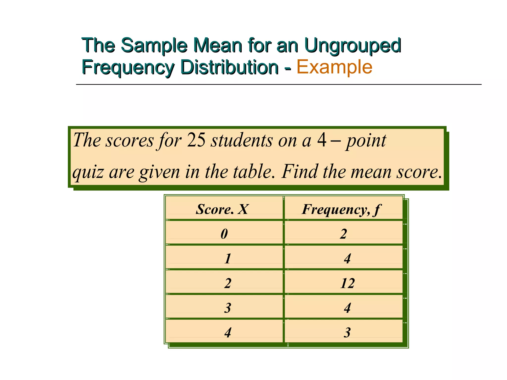
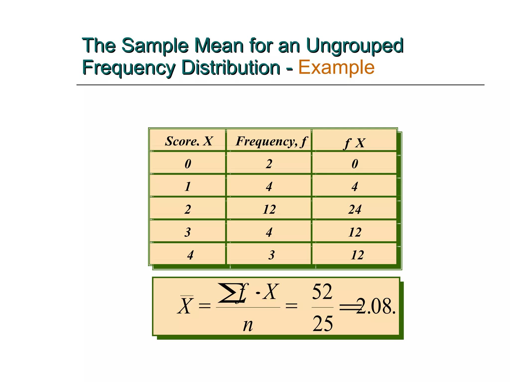
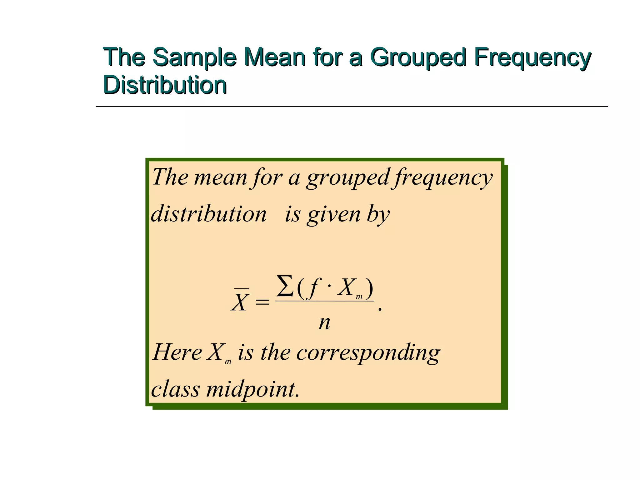
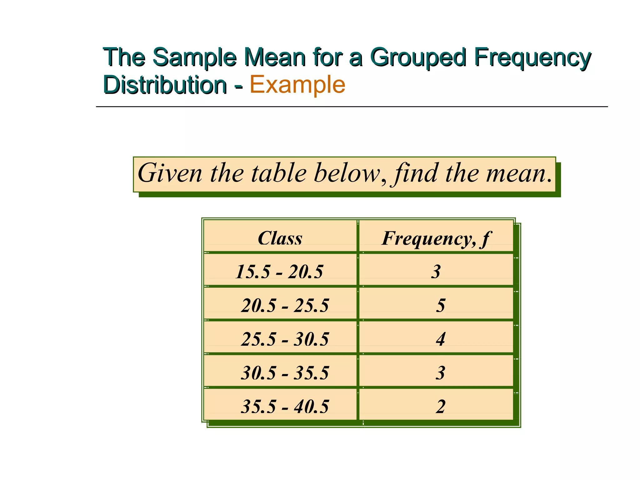
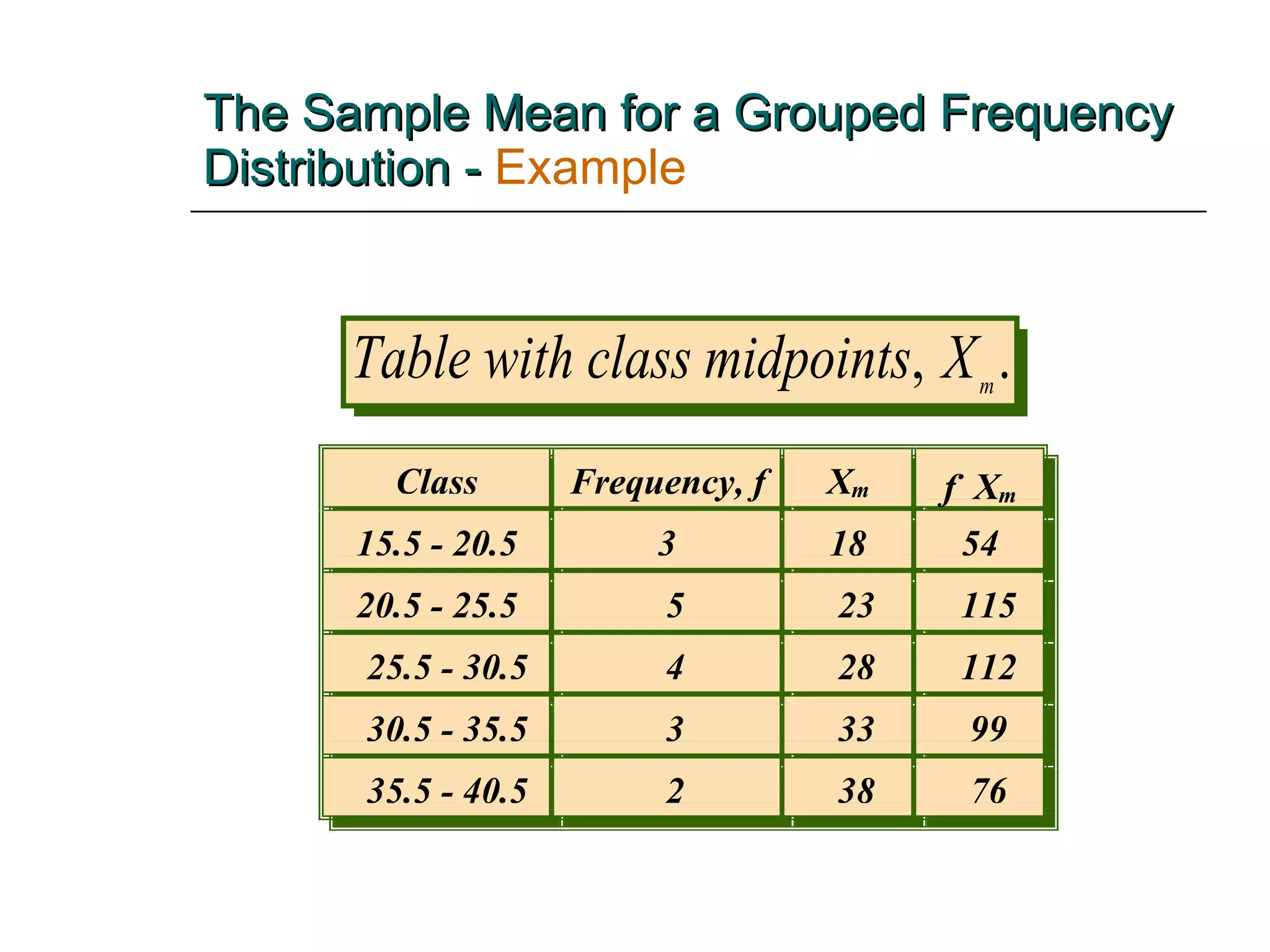
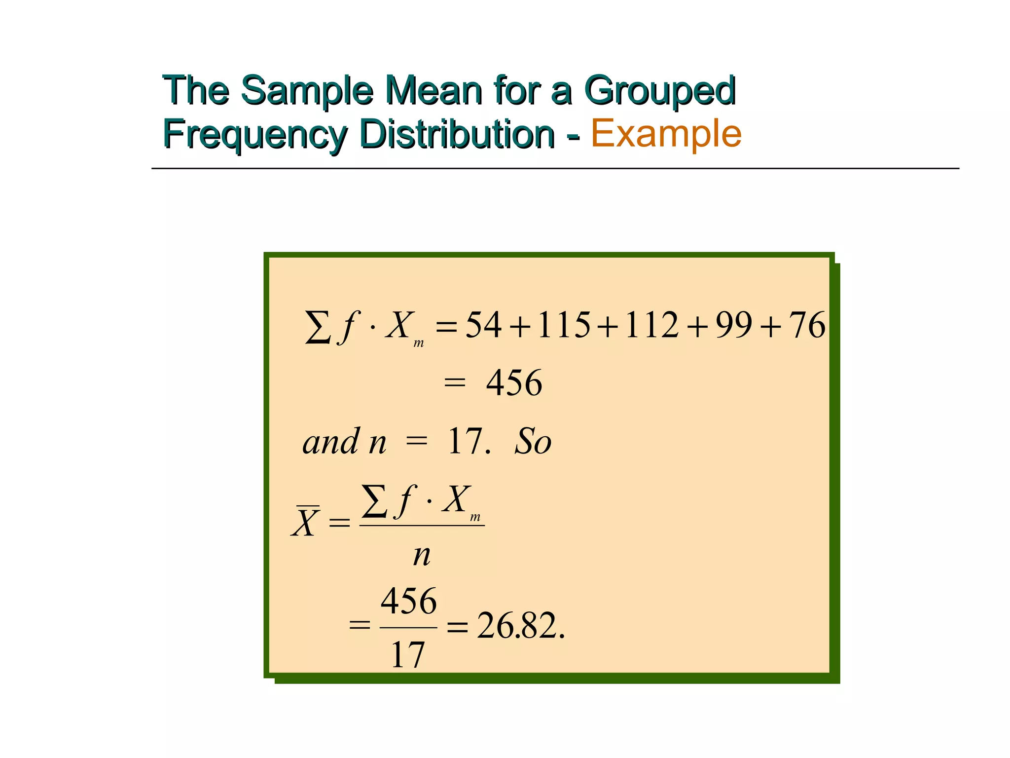
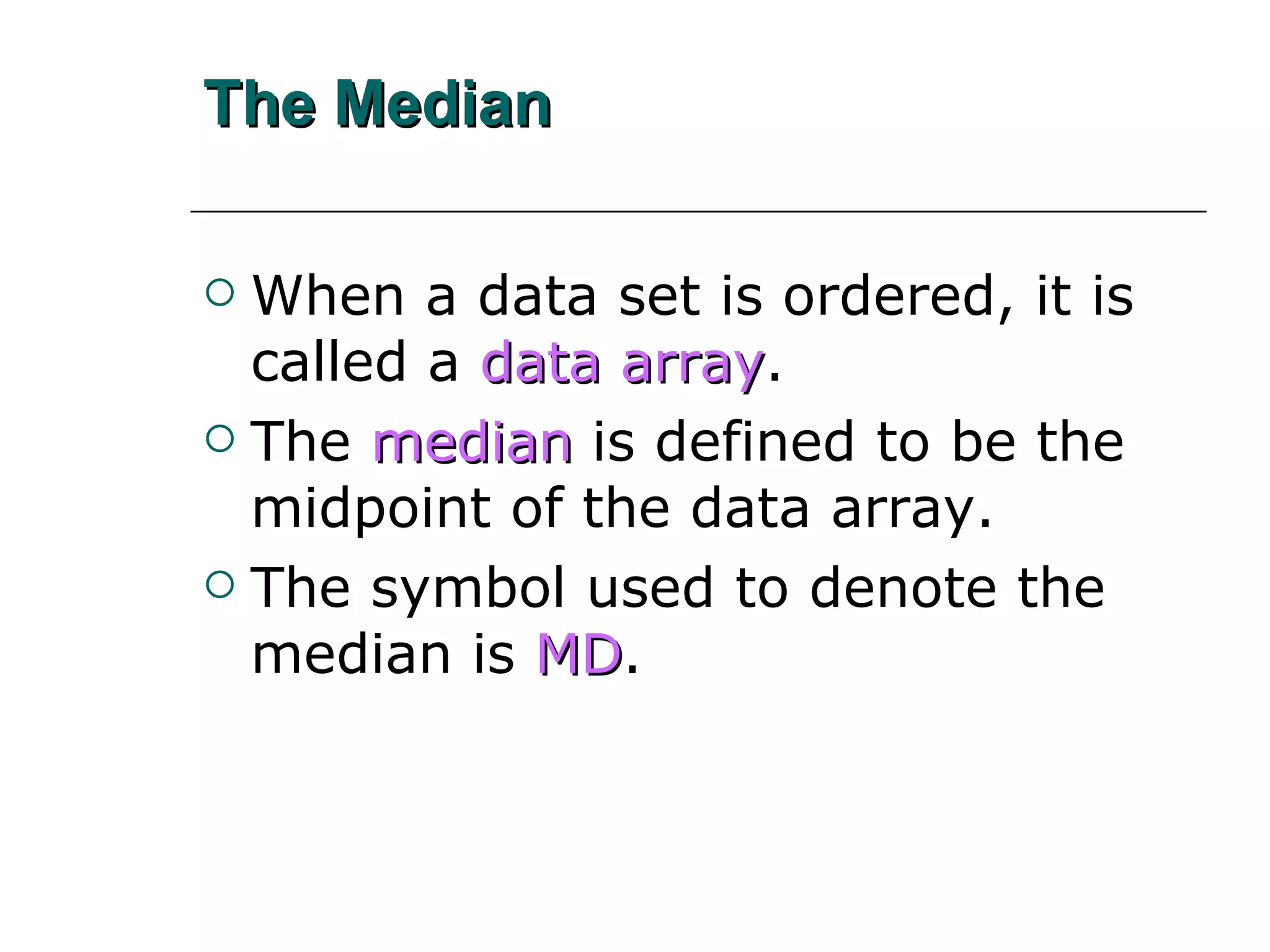
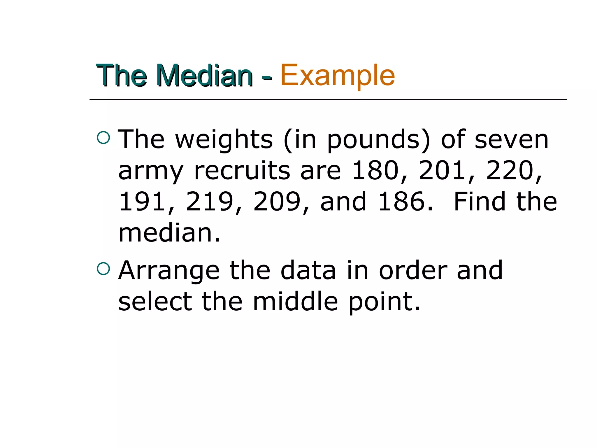
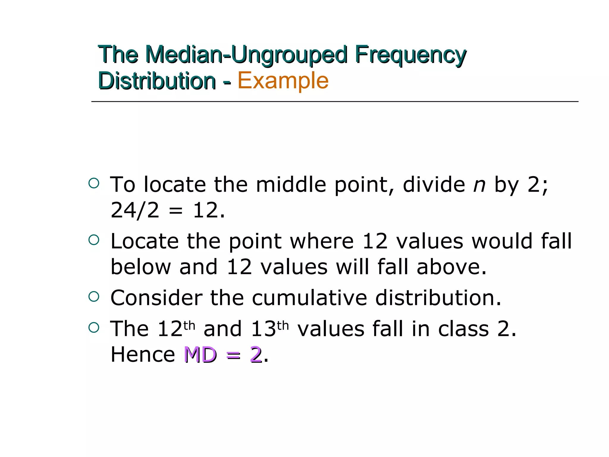
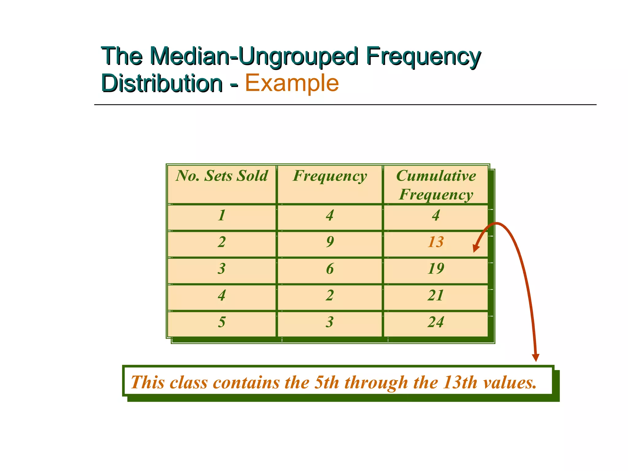
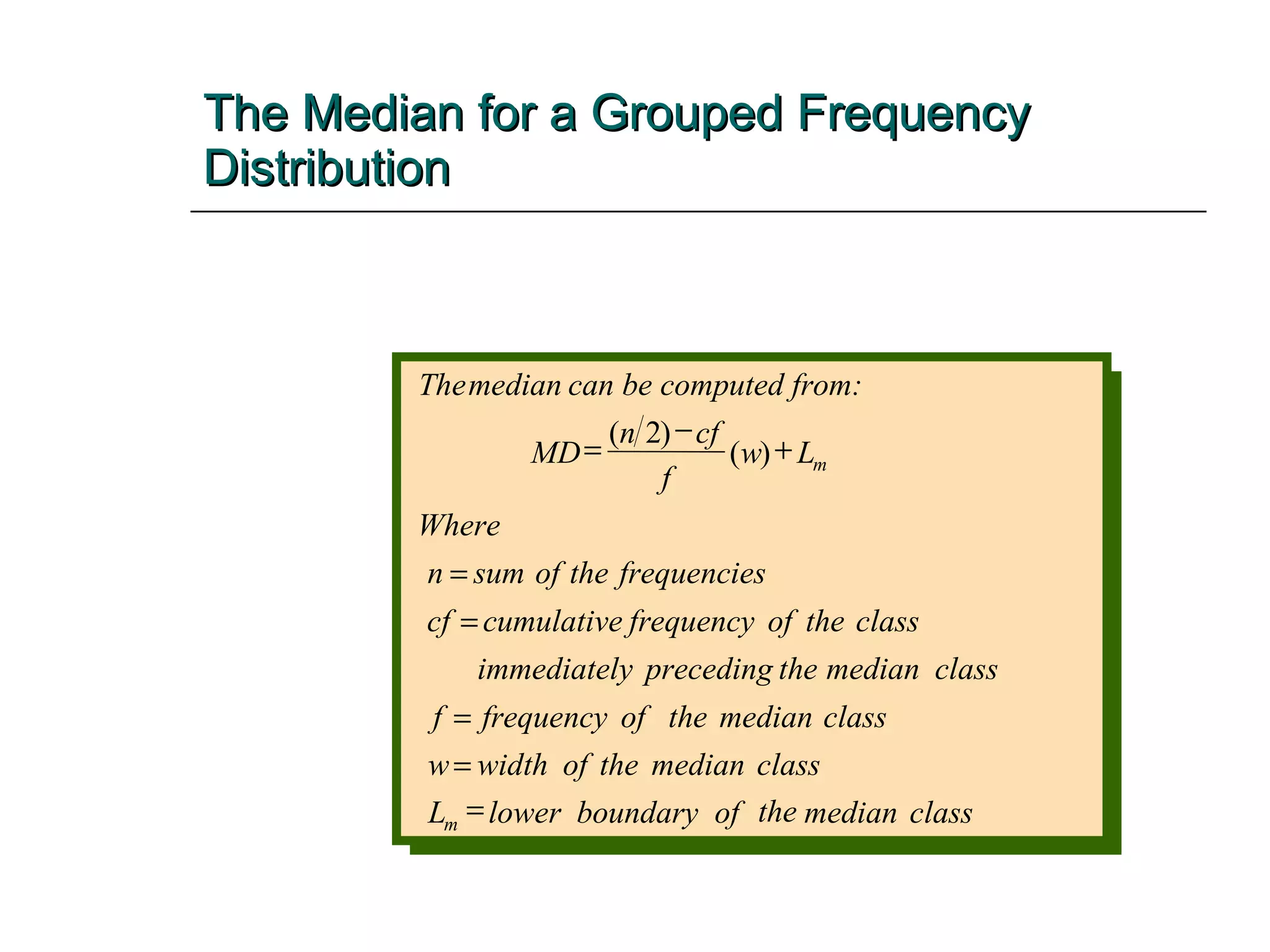
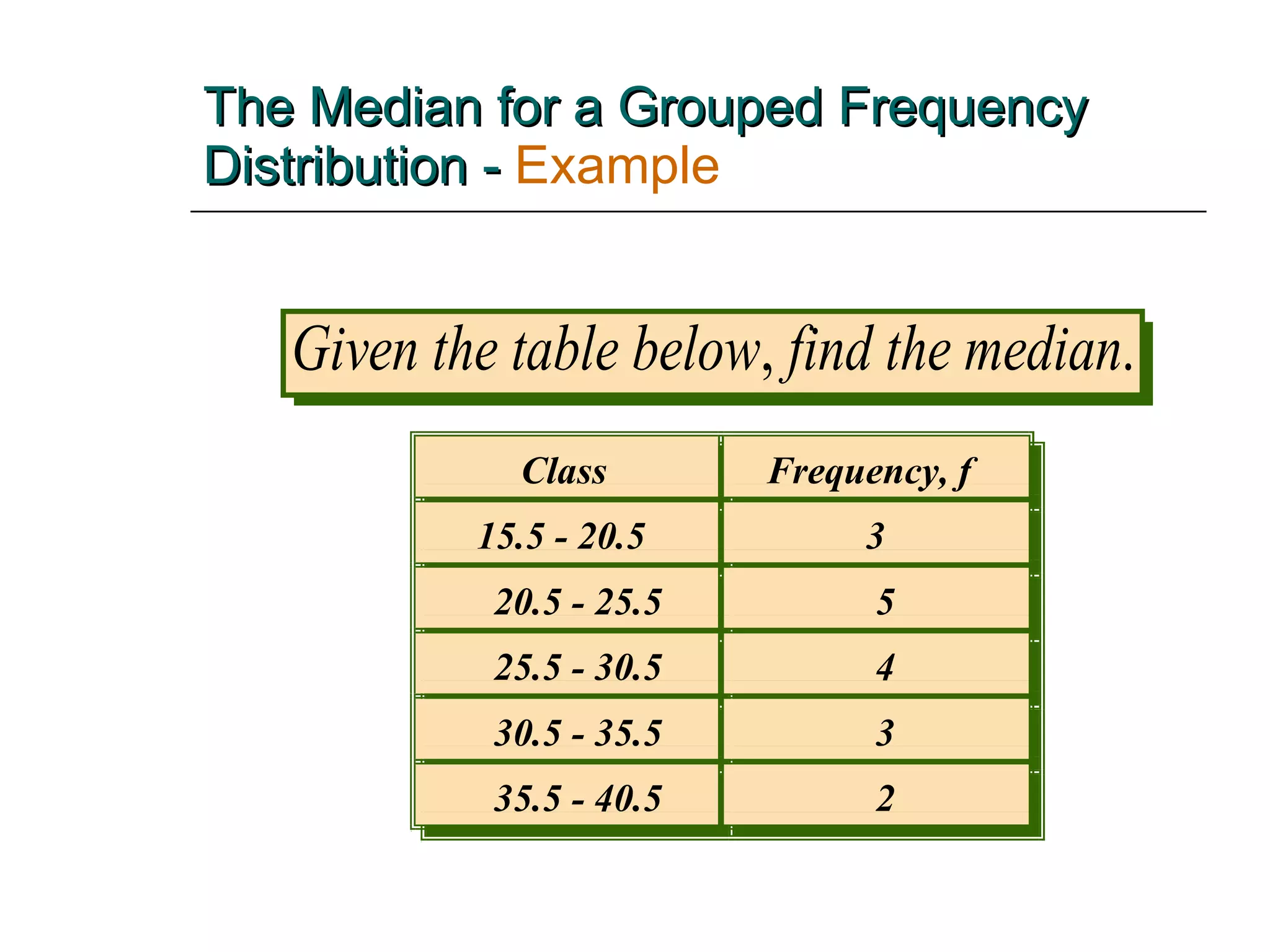
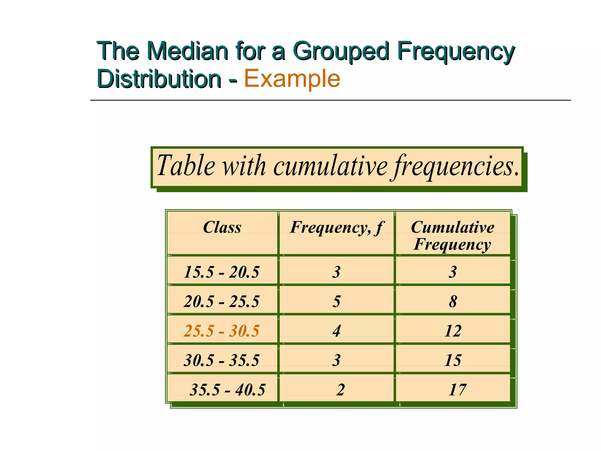
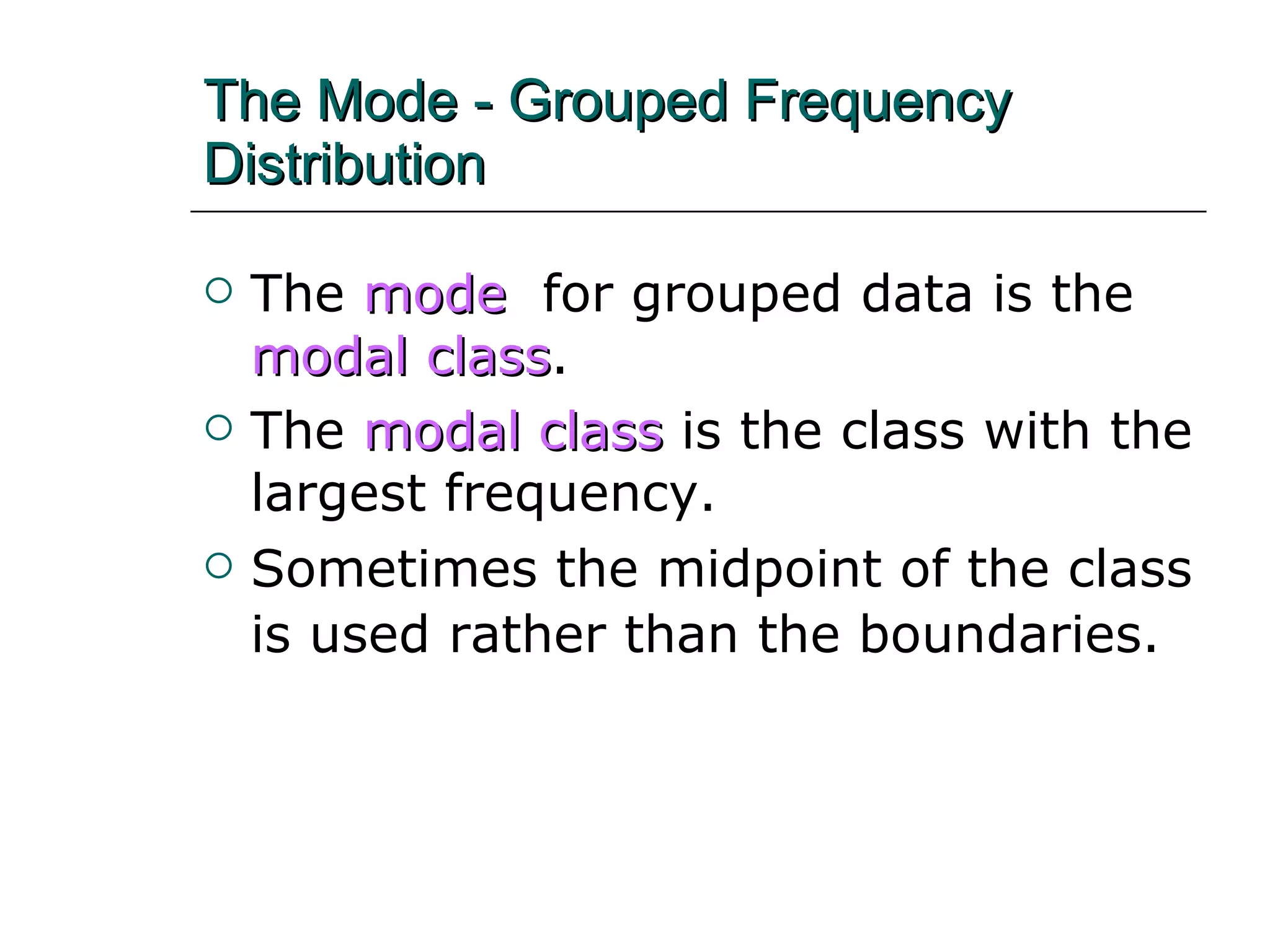
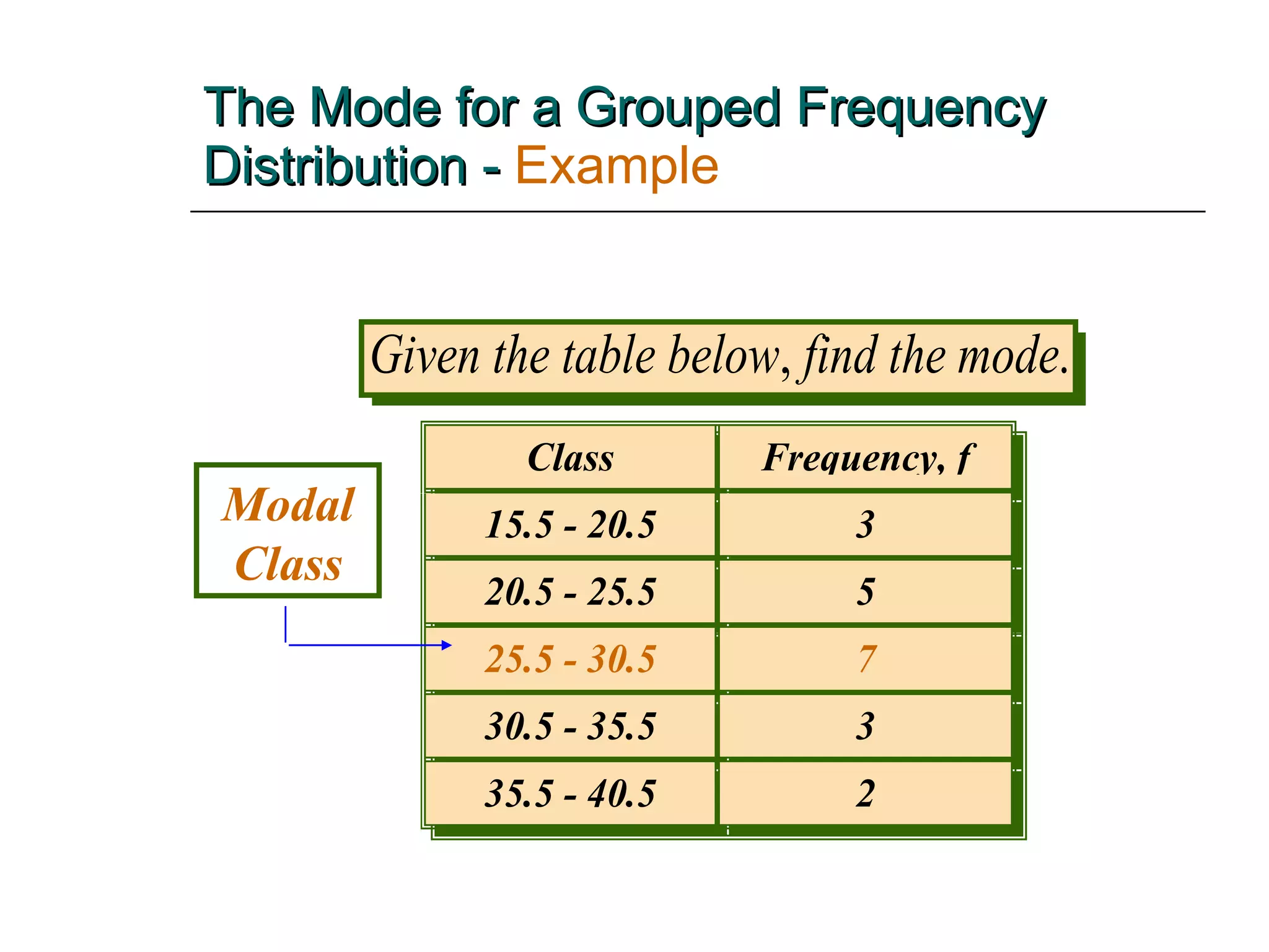
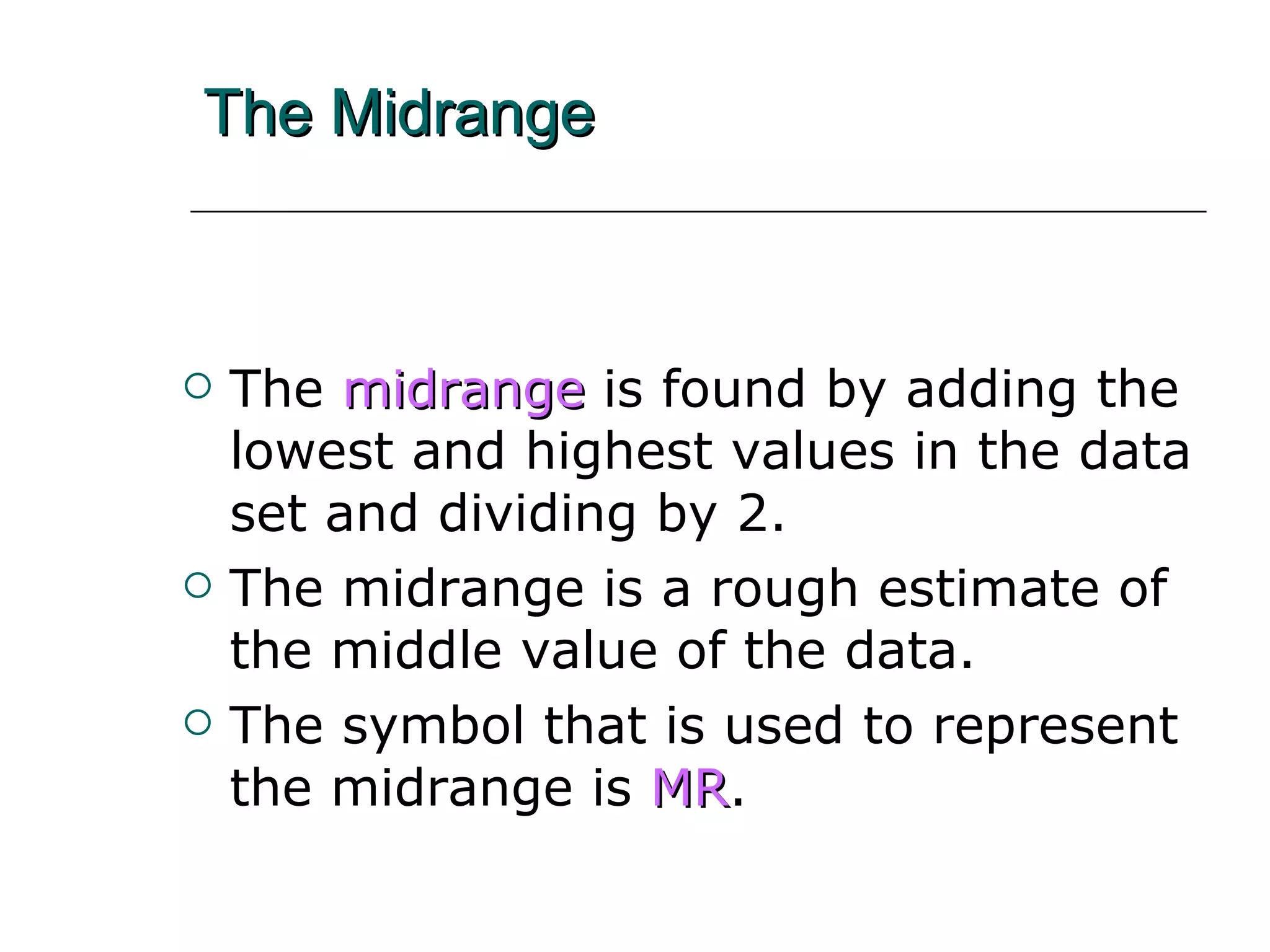
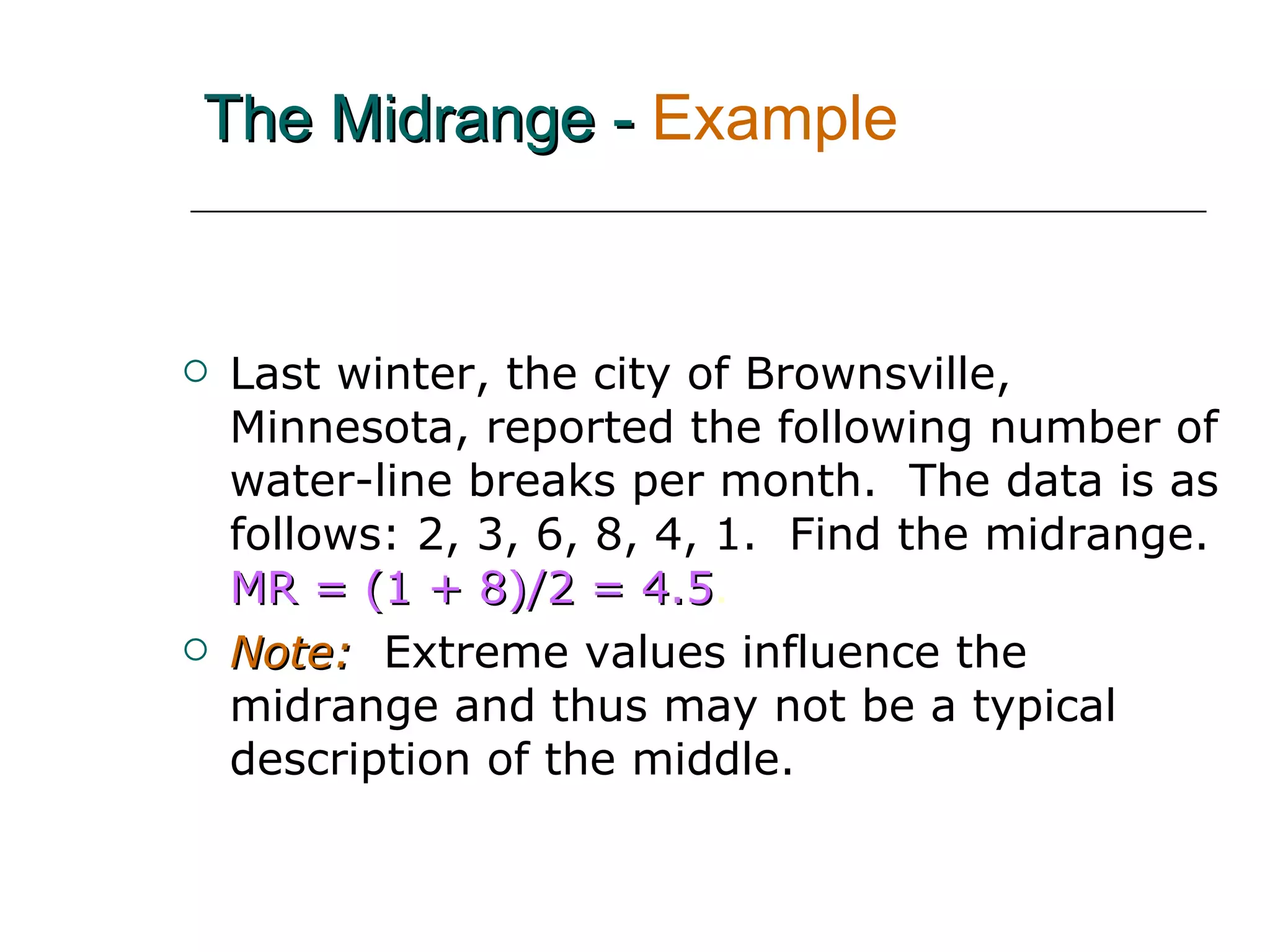
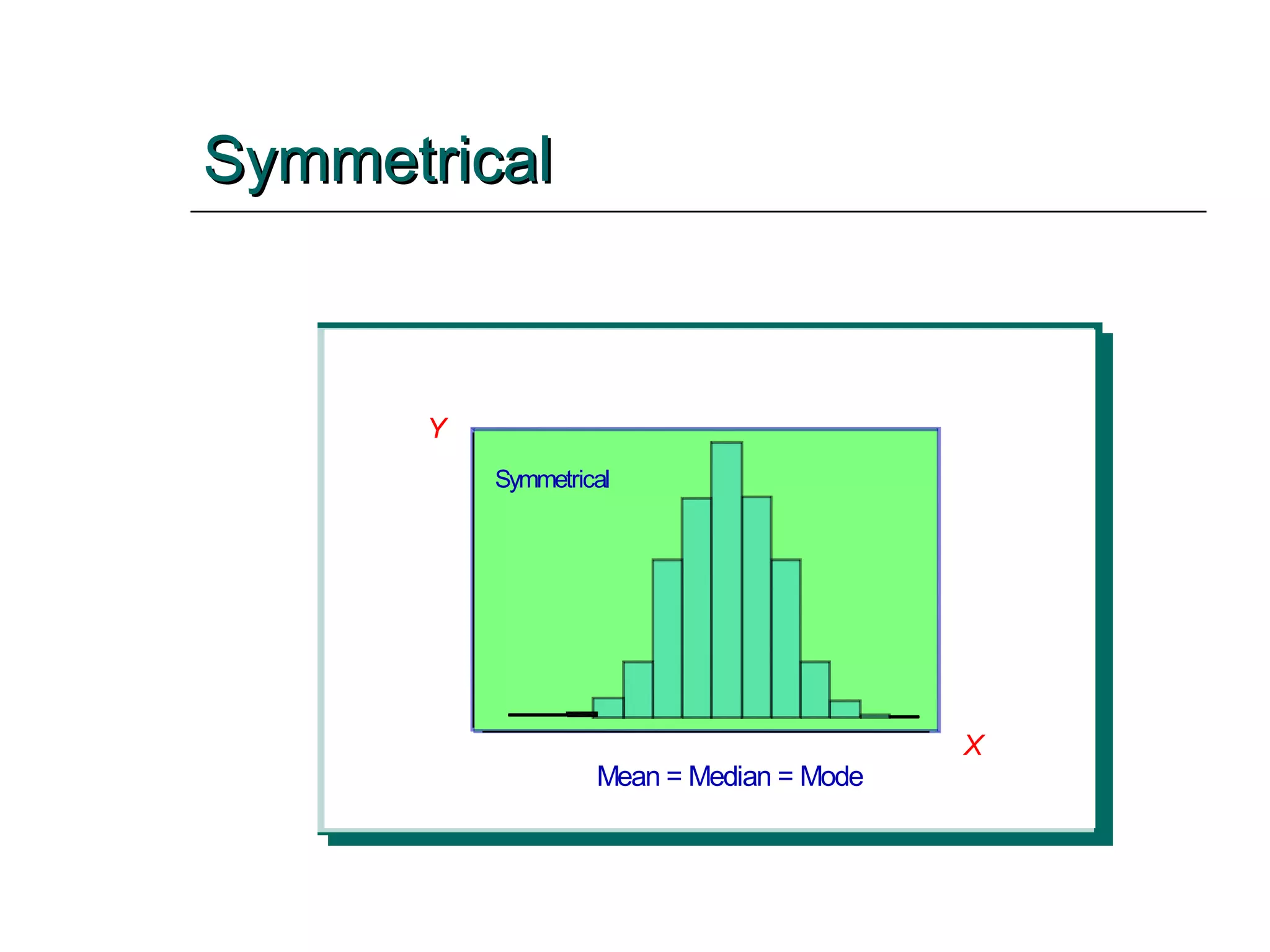
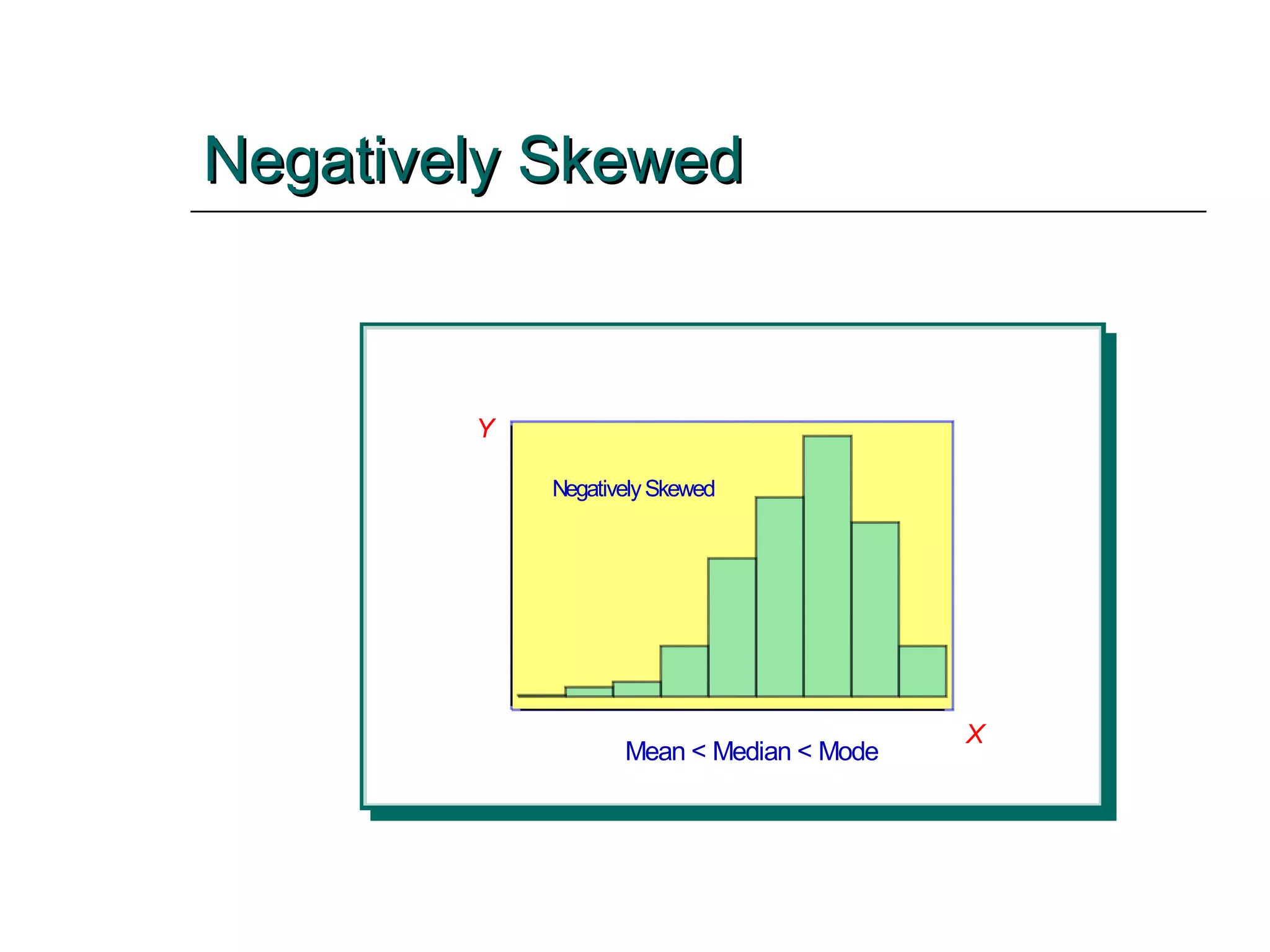
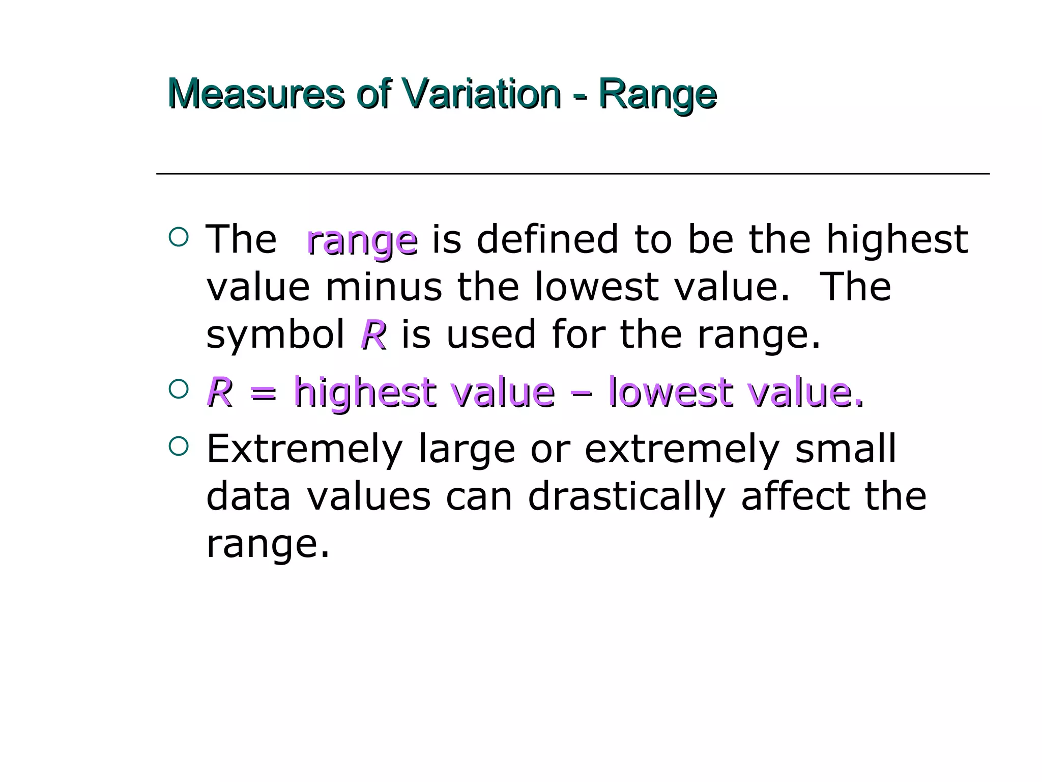
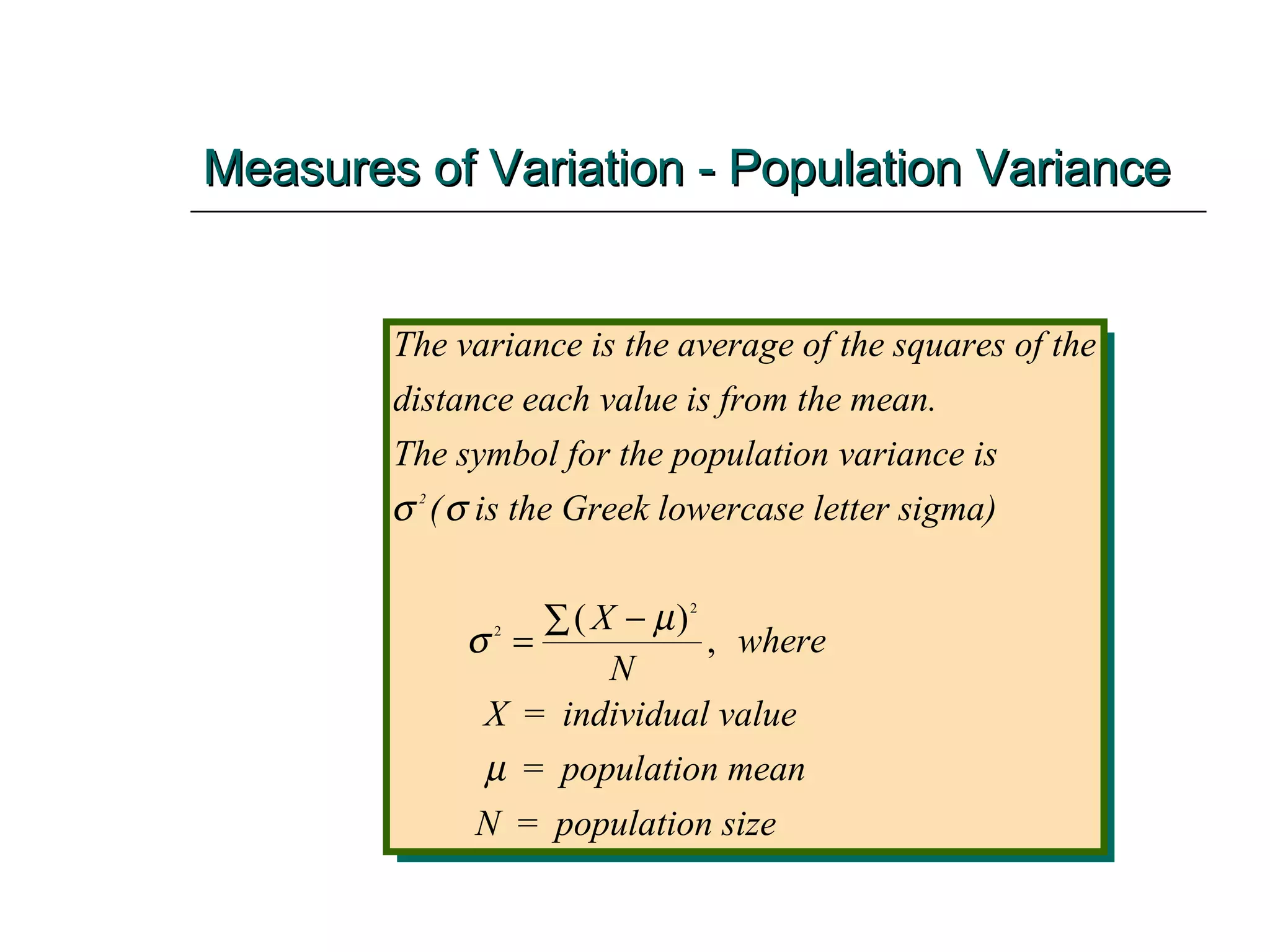
This document provides an overview of key concepts for describing and summarizing data, including measures of central tendency (mean, median, mode), measures of variation (range, variance, standard deviation), and concepts like skewness. It discusses how to calculate and interpret these measures for both grouped and ungrouped data sets. Examples are provided to demonstrate calculating these statistics for different types of data distributions.

1. Chapter 3 Data Description Reference: Allan G. Bluman (2007) Elementary Statistics: A Step-by Step Approach . New York : McGraw Hill

2. Objectives Summarize data using the measures of central tendency, such as the mean, median, mode, and midrange. Describe data using the measures of variation, such as the range, variance, and standard deviation. Identify the position of a data value in a data set using various measures of position, such as percentiles, deciles and quartiles. Use the techniques of exploratory data analysis, including stem and leaf plots, box plots, and five-number summaries to discover various aspects of data.

3. Measures of Central Tendency A statistic is a characteristic or measure obtained by using the data values from a sample. A parameter is a characteristic or measure obtained by using the data values from a specific population.

4. The Mean (arithmetic average) The mean is defined to be the sum of the data values divided by the total number of values. We will compute two means: one for the sample and one for a finite population of values.

5. The Sample Mean

6. The Sample Mean - Example

7. The Population Mean

8. The Population Mean - Example

9. The Sample Mean for an Ungrouped Frequency Distribution The mean for a ungrouped frequency distribution is given by X f X n = ( )  

10. The Sample Mean for an Ungrouped Frequency Distribution - Example Score, X Frequency, f 0 2 1 4 2 12 3 4 4 3 5 Score, X 0 2 1 4 2 12 3 4 4 3 5 Frequency, f

11. The Sample Mean for an Ungrouped Frequency Distribution - Example 5 Score, X  X 0 2 0 1 4 4 2 12 24 3 4 12 4 3 12 5 Frequency, f f Score, X Frequency, f f  X 0 2 0 1 4 4 2 12 24 3 4 12 4 3 12

12. The Sample Mean for a Grouped Frequency Distribution The mean for a grouped frequency distribution is given by X f X n Here X is the correspond ing class midpoint. m m = ( )   .

13. The Sample Mean for a Grouped Frequency Distribution - Example Class Frequency, f 15.5 - 20.5 3 20.5 - 25.5 5 25.5 - 30.5 4 30.5 - 35.5 3 35.5 - 40.5 2 5 Class 15.5 - 20.5 3 20.5 - 25.5 5 25.5 - 30.5 4 30.5 - 35.5 3 35.5 - 40.5 2 5 Frequency, f

14. The Sample Mean for a Grouped Frequency Distribution - Example 35.5 - 40.5 2 38 76 5 Class X  X 15.5 - 20.5 3 18 54 20.5 - 25.5 5 Frequency, f m f m Class Frequency, f X m f  X m 15.5 - 20.5 3 18 54 20.5 - 25.5 5 23 115 25.5 - 30.5 4 28 112 30.5 - 35.5 3 33 99 5 23 115 25.5 - 30.5 4 28 112 30.5 - 35.5 3 33 99 35.5 - 40.5 2 38 76

15. The Sample Mean for a Grouped Frequency Distribution - Example

16. The Median When a data set is ordered, it is called a data array . The median is defined to be the midpoint of the data array. The symbol used to denote the median is MD .

17. The Median - Example The weights (in pounds) of seven army recruits are 180, 201, 220, 191, 219, 209, and 186. Find the median. Arrange the data in order and select the middle point.

18. The Median - Example Data array: 180, 186, 191, 201 , 209, 219, 220. The median, MD = 201 .

19. The Median In the previous example, there was an odd number of values in the data set. In this case it is easy to select the middle number in the data array.

20. The Median When there is an even number of values in the data set, the median is obtained by taking the average of the two middle numbers .

21. The Median - Example Six customers purchased the following number of magazines: 1, 7, 3, 2, 3, 4. Find the median. Arrange the data in order and compute the middle point. Data array: 1, 2, 3, 3, 4, 7. The median, MD = (3 + 3)/2 = 3.

22. The Median - Example The ages of 10 college students are: 18, 24, 20, 35, 19, 23, 26, 23, 19, 20. Find the median. Arrange the data in order and compute the middle point.

23. The Median - Example Data array: 18, 19, 19, 20, 20 , 23 , 23, 24, 26, 35. The median, MD = (20 + 23)/2 = 21.5.

24. The Median-Ungrouped Frequency Distribution For an ungrouped frequency distribution, find the median by examining the cumulative frequencies to locate the middle value.

25. The Median-Ungrouped Frequency Distribution If n is the sample size, compute n /2. Locate the data point where n /2 values fall below and n /2 values fall above.

26. The Median-Ungrouped Frequency Distribution - Example LRJ Appliance recorded the number of VCRs sold per week over a one-year period. The data is given below. No. Sets Sold Frequency 1 4 2 9 3 6 4 2 5 3 No. Sets Sold 1 4 2 9 3 6 4 2 5 3 Frequency

27. The Median-Ungrouped Frequency Distribution - Example To locate the middle point, divide n by 2; 24/2 = 12. Locate the point where 12 values would fall below and 12 values will fall above. Consider the cumulative distribution. The 12 th and 13 th values fall in class 2. Hence MD = 2 .

28. The Median-Ungrouped Frequency Distribution - Example This class contains the 5th through the 13th values.

29. The Median for a Grouped Frequency Distribution class median the of boundary lower L class median the of width w class median the of frequency f class median the preceding immediately class the of frequency cumulative cf frequencies the of sum n Where L w f cf n MD can be computed from: median The m m     ) ( ) 2 (    

30. The Median for a Grouped Frequency Distribution - Example Class Frequency, f 15.5 - 20.5 3 20.5 - 25.5 5 25.5 - 30.5 4 30.5 - 35.5 3 35.5 - 40.5 2 5 Class 15.5 - 20.5 3 20.5 - 25.5 5 25.5 - 30.5 4 30.5 - 35.5 3 35.5 - 40.5 2 5 Frequency, f

31. The Median for a Grouped Frequency Distribution - Example 5 Class Cumulative 15.5 - 20.5 3 3 20.5 - 25.5 5 8 25.5 - 30.5 4 12 30.5 - 35.5 3 15 35.5 - 40.5 2 17 5 Frequency, f Frequency Class Frequency, f Cumulative Frequency 15.5 - 20.5 3 3 20.5 - 25.5 5 8 25.5 - 30.5 4 12 30.5 - 35.5 3 15 35.5 - 40.5 2 17

32. To locate the halfway point, divide n by 2; 17/2 = 8.5  9. Find the class that contains the 9 th value. This will be the median class . Consider the cumulative distribution. The median class will then be 25.5 – 30.5 . The Median for a Grouped Frequency Distribution - Example

33. The Median for a Grouped Frequency Distribution = 17 = = = – 20.5 = 5 ( ) ( ) = (17 / 2) – 8 4 = 26.125. n cf f w L MD n cf f w L m m 8 4 25.5 25 5 2 5 25 5      . ( ) .

34. The Mode The mode is defined to be the value that occurs most often in a data set. A data set can have more than one mode. A data set is said to have no mode if all values occur with equal frequency.

35. The Mode - Examples The following data represent the duration (in days) of U.S. space shuttle voyages for the years 1992-94. Find the mode. Data set: 8, 9, 9, 14, 8, 8, 10, 7, 6, 9, 7, 8, 10, 14, 11, 8, 14, 11. Ordered set: 6, 7, 7, 8, 8, 8, 8, 8, 9, 9, 9, 10, 10, 11, 11, 14, 14, 14. Mode = 8 .

36. The Mode - Examples Six strains of bacteria were tested to see how long they could remain alive outside their normal environment. The time, in minutes, is given below. Find the mode. Data set: 2, 3, 5, 7, 8, 10. There is no mode since each data value occurs equally with a frequency of one.

37. The Mode - Examples Eleven different automobiles were tested at a speed of 15 mph for stopping distances. The distance, in feet, is given below. Find the mode. Data set: 15, 18, 18, 18, 20, 22, 24, 24, 24, 26, 26. There are two modes (bimodal) . The values are 18 and 24 . Why?

38. The Mode for an Ungrouped Frequency Distribution - Example Values Frequency, f 15 3 20 5 25 8 30 3 35 2 5 Values 15 3 20 5 25 8 30 3 35 2 5 Mode Frequency, f

39. The Mode - Grouped Frequency Distribution The mode for grouped data is the modal class . The modal class is the class with the largest frequency. Sometimes the midpoint of the class is used rather than the boundaries.

40. The Mode for a Grouped Frequency Distribution - Example Modal Class

41. The Midrange The midrange is found by adding the lowest and highest values in the data set and dividing by 2. The midrange is a rough estimate of the middle value of the data. The symbol that is used to represent the midrange is MR .

42. The Midrange - Example Last winter, the city of Brownsville, Minnesota, reported the following number of water-line breaks per month. The data is as follows: 2, 3, 6, 8, 4, 1. Find the midrange. MR = (1 + 8)/2 = 4.5 . Note: Extreme values influence the midrange and thus may not be a typical description of the middle.

43. The Weighted Mean The weighted mean is used when the values in a data set are not all equally represented. The weighted mean of a variable X is found by multiplying each value by its corresponding weight and dividing the sum of the products by the sum of the weights.

44. The Weighted Mean

45. Distribution Shapes Frequency distributions can assume many shapes. The three most important shapes are positively skewed , symmetrical , and negatively skewed .

46. Positively Skewed X Y M o d e < M e d i a n < M e a n P o s i t i v e l y S k e w e d

47. Symmetrical n Y X S y m m e t r i c a l M e a n = M e d i a = M o d e

48. Negatively Skewed < M e d i a n < M o d e Y X N e g a t i v e l y S k e w e d M e a n

49. Measures of Variation - Range The range is defined to be the highest value minus the lowest value. The symbol R is used for the range. R = highest value – lowest value. Extremely large or extremely small data values can drastically affect the range.

50. Measures of Variation - Population Variance

51. Measures of Variation - Population Standard Deviation

52. Consider the following data to constitute the population: 10, 60, 50, 30, 40, 20. Find the mean and variance. The mean  = (10 + 60 + 50 + 30 + 40 + 20)/6 = 210/6 = 35. The variance  2 = 1750/6 = 291.67. See next slide for computations. Measures of Variation - Example

53. Measures of Variation - Example

54. Measures of Variation - Sample Variance The unbias ed estimat or of the population variance o r the samp le varianc e is a statistic whose valu e approxim ates the expected v alue of a population variance. It is deno ted by s 2 , ( ) , where s X X n and X sample mean n sample size = = 2 2 1    

55. Measures of Variation - Sample Standard Deviation The sample standard deviation is the squ are root of t he sample variance. = 2 s s X X n     ( ) . 2 1

56. Shortcut Formula for the Sample Variance and the Standard Deviation = = X X n n s X X n n 2 2 2 2 1 1         ( ) / ( ) / s 2

57. Find the variance and standard deviation for the following sample: 16, 19, 15, 15, 14.  X = 16 + 19 + 15 + 15 + 14 = 79.  X 2 = 16 2 + 19 2 + 15 2 + 15 2 + 14 2 = 1263. Sample Variance - Example

58. Sample Variance - Example = 1263  (79) = 3.7 = 3.7 2 s X X n n s 2 2 2 1 5 4 1 9       ( ) / / . .

59. For grouped data, use the class midpoints for the observed value in the different classes. For ungrouped data, use the same formula (see next slide) with the class midpoints, X m , replaced with the actual observed X value. Sample Variance for Grouped and Ungrouped Data

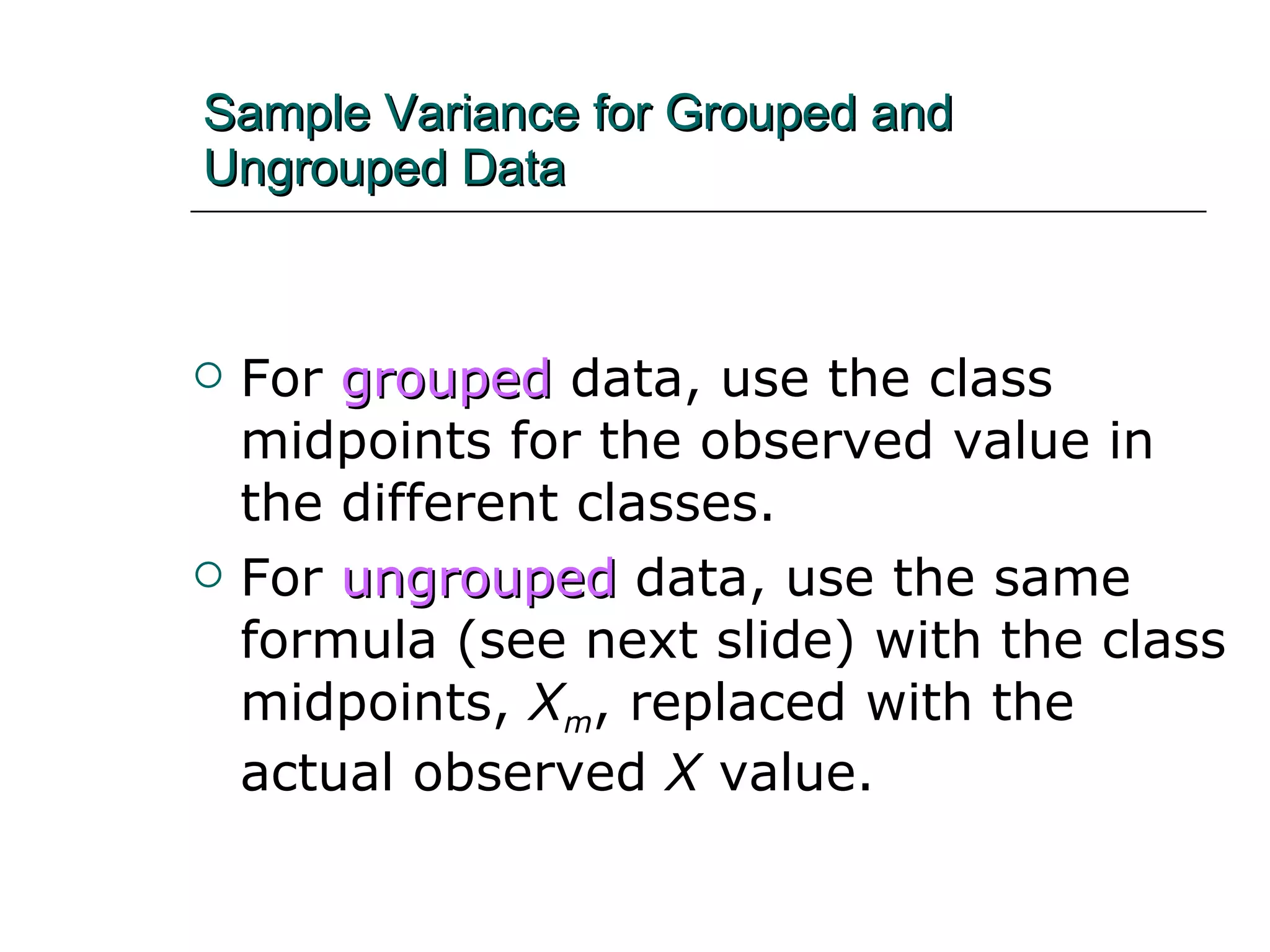
60. Sample Variance for Grouped and Ungrouped Data The sample variance for groupe d data: = s f X f X n n m m 2 2 2 1       [( ) / ] . For ungrouped data, replace X m with the observe X value.

61. Sample Variance for Ungrouped Data - Example X f f  X f  X 2 5 2 10 50 6 3 18 108 7 8 56 392 8 1 8 64 9 6 54 486 10 4 40 400 n = 24  f  X = 186  f  X 2 = 1500 X f f  X f  X 2 5 2 10 50 6 3 18 108 7 8 56 392 8 1 8 64 9 6 54 486 10 4 40 400 n = 24  f  X = 186  f  X 2 = 1500

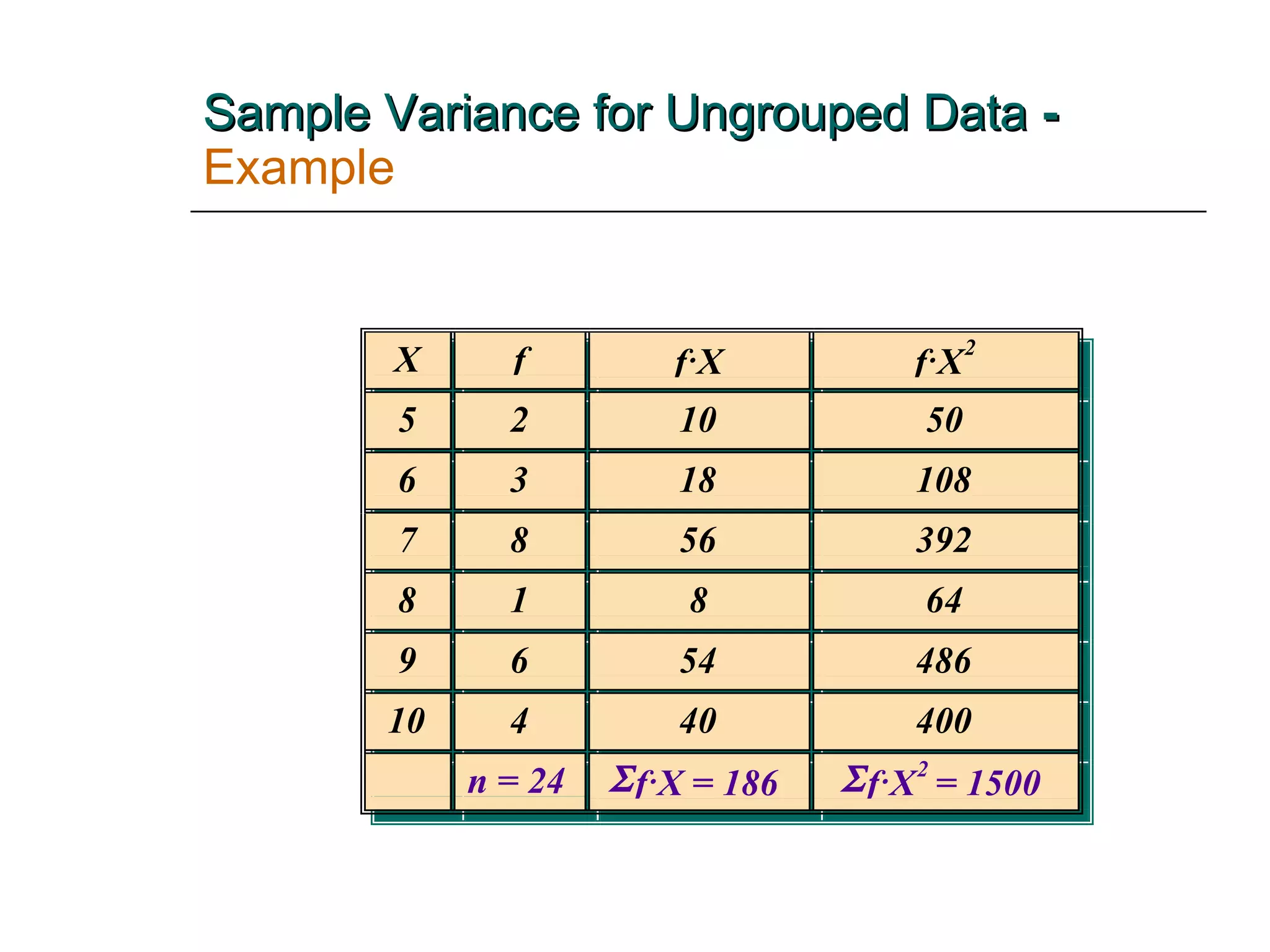
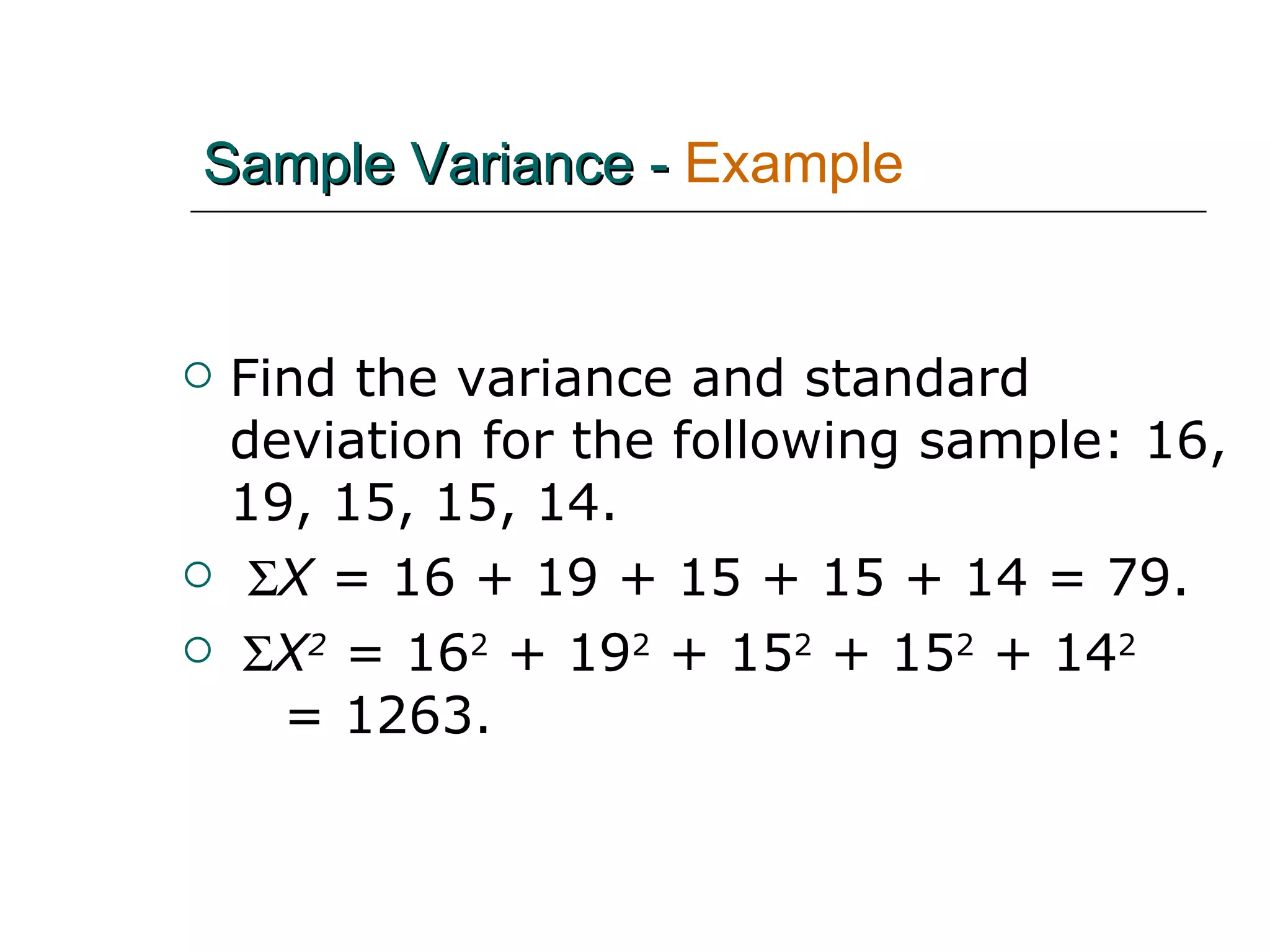
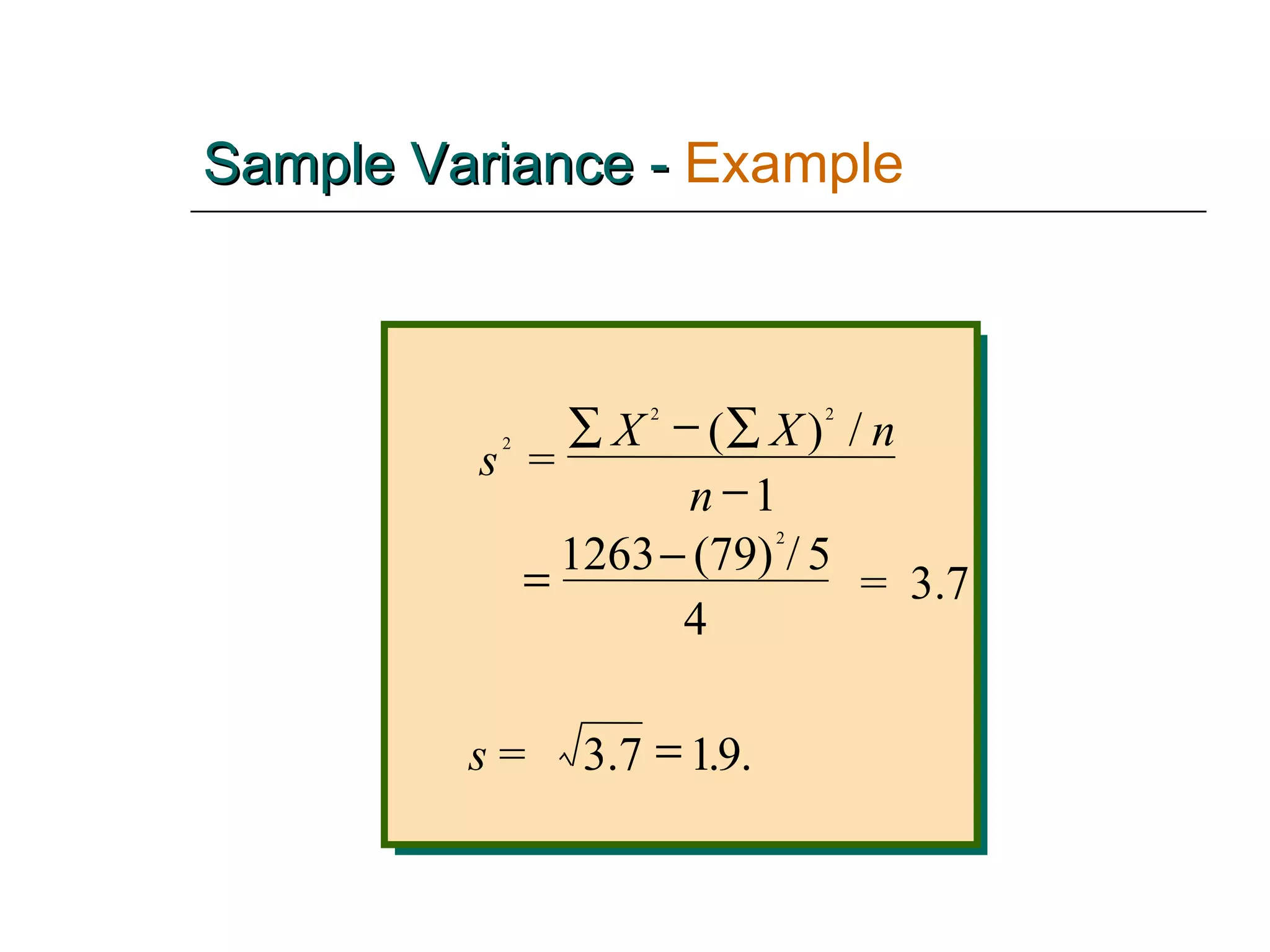
62. Sample Variance for Ungrouped Data - Example The sample variance and standa rd deviati on: = = 1500  [(186) 2 s f X f X n n s 2 2 2 1 24 23 2 54 2 54 1 6          [( ) / ] / ] . . . . .

63. The coefficient of variation is defined to be the standard deviation divided by the mean. The result is expressed as a percentage. Coefficient of Variation CVar s X or CVar    100% 100%. =  

64. Example : The mean of the number of sales of cars over a 3-month period is 87 and the standard deviation is 5. The mean of the commissions is $5225 and the standard deviation is $773. Compare the variations of the two. The coefficient of variation are sales commissions Since the coefficient of variation is larger for commissions, the commissions are more variable than sales. Coefficient of Variation

65. Chebyshev’s Theorem The proportion of values from a data set that will fall within k standard deviations of the mean will be at least 1 – 1/ k 2 , where k is any number greater than 1. For k = 2, 75% of the values will lie within 2 standard deviations of the mean. For k = 3, approximately 89% will lie within 3 standard deviations.

66. Chebyshev’s Theorem Example : The mean price of houses in a certain neighbourhood is $50 000 and the standard deviation is $10 000. Find the price range for which at least 75% of the houses will sell. Chebyshev’s theorem states that three-fourths or 75% of the data values will fall within 2 standard deviations of the mean. Thus, $50 000 + 2($10 000) = $50 000 + $20 000 = $70 000 and $50 000 – 2($10 000) = $50 000 – $20 000 = $30 000 Hence, at least 75% of all homes sold in the area will have a price range from $30 000 to $70 000.

67. The Empirical (Normal) Rule For any bell shaped distribution: Approximately 68% of the data values will fall within one standard deviation of the mean. Approximately 95% will fall within two standard deviations of the mean. Approximately 99.7% will fall within three standard deviations of the mean.

68. The Empirical (Normal) Rule        -- 95%                                

69. Measures of Position — z score The standard score or z score for a value is obtained by subtracting the mean from the value and dividing the result by the standard deviation. The symbol z is used for the z score .

70. The z score represents the number of standard deviations a data value falls above or below the mean. Measures of Position — z-score For samples z X X s For population s z X : . : .      

71. A student scored 65 on a statistics exam that had a mean of 50 and a standard deviation of 10. He score 30 on a history test with a mean of 25 and a standard deviation of 5. Compute the z -score. z (for statistics) = (65 – 50)/10 = 1.5. z (for history) = (30 – 25)/5 = 1.0 That is, the score of 65 is 1.5 standard deviations above the mean. Since the z score for statistics is larger, his relative position in statistics class is higher than his relative position in the history class. If the z score is positive, the score is above the mean. If the z score is 0, the score is the same as the mean. If the z score is negative, the score is below the mean. z-score - Example

72. Measures of Position - Percentiles Percentiles divide the distribution into 100 groups. The P k percentile is defined to be that numerical value such that at most k % of the values are smaller than P k and at most (100 – k )% are larger than P k in an ordered data set.

73. Percentile Formula The percentile corresponding to a given value ( X ) is computed by using the formula: Percentile number of values below X + 0.5 total number of values   100%

74. Percentiles - Example A teacher gives a 20-point test to 10 students. Find the percentile rank of a score of 12. Scores: 18, 15, 12, 6, 8, 2, 3, 5, 20, 10. Ordered set: 2, 3, 5, 6, 8, 10, 12, 15, 18, 20. Percentile = [(6 + 0.5)/10](100%) = 65th percentile. Student did better than 65% of the class.

75. Percentiles - Finding the value Corresponding to a Given Percentile Procedure: Let p be the percentile and n the sample size. Step 1: Arrange the data in order. Step 2: Compute c = ( n  p )/100 . where n = total number of values p = percentile Step 3: If c is not a whole number, round up to the next whole number. If c is a whole number, use the value halfway between c and c +1 .

76. Percentiles - Finding the value Corresponding to a Given Percentile Step 4: The value of c is the position value of the required percentile. Example: Find the value of the 25th percentile for the following data set: 2, 3, 5, 6, 8, 10, 12, 15, 18, 20. Note: the data set is already ordered. n = 10, p = 25, so c = (10  25)/100 = 2.5. Hence round up to c = 3 . Thus, the value of the 25th percentile is the value X = 5.

77. Percentiles - Finding the value Corresponding to a Given Percentile Find the 80th percentile. c = (10  80)/100 = 8. Thus the value of the 80th percentile is the average of the 8th and 9th values. Thus, the 80th percentile for the data set is (15 + 18)/2 = 16.5.

78. Special Percentiles - Deciles and Quartiles Deciles divide the data set into 10 groups. Deciles are denoted by D 1 , D 2 , …, D 9 with the corresponding percentiles being P 10 , P 20 , …, P 90 Quartiles divide the data set into 4 groups.

79. Special Percentiles - Deciles and Quartiles Quartiles are denoted by Q 1 , Q 2 , and Q 3 with the corresponding percentiles being P 25 , P 50 , and P 75 . The median is the same as P 50 or Q 2 .

80. Special Percentiles - Quartiles Finding Data Values Corresponding to Q 1 , Q 2 and Q 3 Step 1: Arrange the data in order from lowest to highest. Step 2: Find the median of the data values. This is the value of Q 2 . Step 3: Find the median of the data values that fall below Q 2 . This is the value of Q 1 . Step 4: Find the median of the data values that fall above Q 2 . This is the value of Q 3 .

81. Outliers and the Interquartile Range (IQR) An outlier is an extremely high or an extremely low data value when compared with the rest of the data values. The Interquartile Range , IQR = Q 3 – Q 1 .

82. Outliers and the Interquartile Range (IQR) To determine whether a data value can be considered as an outlier: Step 1: Compute Q 1 and Q 3 . Step 2: Find the IQR = Q 3 – Q 1 . Step 3: Compute (1.5)(IQR). Step 4: Compute Q 1 – (1.5)(IQR) and Q 3 + (1.5)(IQR).

83. Outliers and the Interquartile Range (IQR) To determine whether a data value can be considered as an outlier: Step 5: Compare the data value (say X) with Q 1 – (1.5)(IQR) and Q 3 + (1.5)(IQR). If X < Q 1 – (1.5)(IQR) or if X > Q 3 + (1.5)(IQR), then X is considered an outlier.

84. Outliers and the Interquartile Range (IQR) - Example Given the data set 5, 6, 12, 13, 15, 18, 22, 50, can the value of 50 be considered as an outlier? Q 1 = 9, Q 3 = 20, IQR = 11. Verify . (1.5)(IQR) = (1.5)(11) = 16.5. 9 – 16.5 = – 7.5 and 20 + 16.5 = 36.5. The value of 50 is outside the range – 7.5 to 36.5, hence 50 is an outlier.

85. Exploratory Data Analysis - Stem and Leaf Plot A stem and leaf plot is a data plot that uses part of a data value as the stem and part of the data value as the leaf to form groups or classes.

86. At an outpatient testing center, a sample of 20 days showed the following number of cardiograms done each day: 25, 31, 20, 32, 13, 14, 43, 02, 57, 23, 36, 32, 33, 32, 44, 32, 52, 44, 51, 45. Construct a stem and leaf plot for the data. Exploratory Data Analysis - Stem and Leaf Plot - Example

87. Exploratory Data Analysis – Stem and Leaf Plot - Example Leading Digit (Stem) Trailing Digit (Leaf) 0 2 1 3 4 2 0 3 5 3 1 2 2 2 2 3 6 4 3 4 4 5 5 1 2 7

88. Exploratory Data Analysis - Box Plot When the data set contains a small number of values, a box plot is used to graphically represent the data set. These plots involve five values: the minimum value , the lower hinge , the median , the upper hinge , and the maximum value .

89. Exploratory Data Analysis - Box Plot The lower hinge is the median of all values less than or equal to the median when the data set has an odd number of values, or as the median of all values less than the median when the data set has an even number of values. The symbol for the lower hinge is LH .

90. Exploratory Data Analysis - Box Plot The upper hinge is the median of all values greater than or equal to the median when the data set has an odd number of values, or as the median of all values greater than the median when the data set has an even number of values. The symbol for the upper hinge is UH .

91. Exploratory Data Analysis - Box Plot - Example (Cardiograms data)

92. Information Obtained from a Box Plot If the median is near the center of the box, the distribution is approximately symmetric. If the median falls to the left of the center of the box, the distribution is positively skewed. If the median falls to the right of the center of the box, the distribution is negatively skewed.

93. Information Obtained from a Box Plot If the lines are about the same length, the distribution is approximately symmetric. If the right line is larger than the left line, the distribution is positively skewed. If the left line is larger than the right line, the distribution is negatively skewed.