SlideShare a Scribd company logo
1 of 186
Download to read offline
Logic and Mathematics
from Classical to 21th Century
Euclid Leibnitz
Godel Pearl
Boole
Simplified for students
Contents
Tools (WolframAlpha and Python)
Classical Western Logic and Mathematics
Non-Western Mathematics
Rebirth of Western Mathematics
Graphing Equations
20th and 21 Century Mathematics
Logic, Sets, and Probability
Causal Models and Reasoning
Advanced Topics:
Causal Reasoning and Deep Learning
Continuous Probability Distributions
This is mostly a basic presentation not requiring calculus
A more advanced set of slides has been added at the end
The simple topics in this presentation (e.g. logic,sets, probability, networks,
algorithms number theory) would provide a more interesting math curriculuum
than geometry, trigonometry, and algebraic manipulation.
Tools
Every student in high school should know WolframAlpha and Python.
WolframAlpha to perform computations and Python to understand programming
WolframAlpha
WolframAlpha Mathematics
Elementary Math
Algebra
Calculus & Analysis
Geometry
Plotting & Graphics
Differential Equations
Numbers
Trigonometry
Linear Algebra
Discrete Mathematics
Number Theory
Complex Analysis
Applied Mathematics
Logic & Set Theory
Mathematical Definitions
Continued Fractions
Statistics
Famous Math Problems
Probability
Python Programming Language
Python is an easy to learn, powerful programming language. It has efficient high-level data
structures and a simple but effective approach to object-oriented programming. Python’s
elegant syntax and dynamic typing, together with its interpreted nature, make it an ideal
language for scripting and rapid application development in many areas on most platforms.
The Python interpreter and the extensive standard library are freely available in source or
binary form for all major platforms from the Python Web site, https://www.python.org/, and
may be freely distributed. The same site also contains distributions of and pointers to many
free third party Python modules, programs and tools, and additional documentation.
The Python interpreter is easily extended with new functions and data types implemented in C
or C++ (or other languages callable from C). Python is also suitable as an extension language
for customizable applications.
This tutorial introduces the reader informally to the basic concepts and features of the Python
language and system. It helps to have a Python interpreter handy for hands-on experience, but
all examples are self-contained, so the tutorial can be read off-line as well.
For a description of standard objects and modules, see The Python Standard Library. The
Python Language Reference gives a more formal definition of the language. To write
extensions in C or C++, read Extending and Embedding the Python Interpreter and Python/C
API Reference Manual. There are also several books covering Python in depth.
Tutorial
Python is an easy to learn powerful programming language. There are many valuable
libraries that provide much additional capabilities. The interpreter is an important
tool for caatching errors.
Python Libraries
Scikit-learn
NuPIC
Ramp
NumPy
Pipenv
TensorFlow
Bob
PyTorch
PyBrain
MILK
Keras
Dash
Pandas
Scipy
Matplotlib
SymPy
Caffe2
Seaborn
Hebel
Chainer
OpenCV Python
Theano
NLTK
SQLAlchemy
Bokeh
Important Python Libraries for Data Science
What is a Library?
Classical Logic and Mathematics
Aristotle’s Logic Aristotle
All Dogs are Animals D -> A
leonard is a Dog l is in D
Conclusion
Given
leonard is a Animal l is in A
Pictures
Not Necessarily True: (Converse) All Animal are Dogs - (Inverse) Not a Dog means Not an Animal
Always True: (Contrapositive) Not an Animal means Not a Dog
Dogs
Animals
True:
All Dogs are Animals Dogs
Animals
Not an Animal mean Not a Dog
False:
All Animals are Dogs
cat
Not a Dog means Not an Animal
(cat is a Counterexample)
Given: Guilty people always tell lies
Test: Which sentence must be true?
If he tell lies then he is guilty
If he is not guilty he won’t tell lies
If he is not telling lies then he is not guilty
Given: Whatever doesn’t kill you makes
you stronger
Contrapositive is true: Whatever
doesn’t make you stronger kills you
What is wrong with this logic?
Aquinas
Proof of God’s Existence by St Thomas Aquinas
St Thomas Aquinas was a follower of Aristotle in 1200 AD.
He believed that the existence of God could be proved by logic
rather than taken on faith. Below is the best of his 5 proofs.
Proof from First Cause: (or what caused the Big Bang?)
1. In the world, we can see that things are caused.
2. But it is not possible for something to be the cause of itself
because this would entail that it exists prior to itself, which is a
contradiction.
3. If that by which it is caused is itself caused, then it too must have
a cause.
4. But this cannot be an infinitely long chain, so, there must be a
cause which is not itself caused by anything further.
5. This everyone understands to be God.
Can you find a flaw in this logic?
Mandala
D C
B
A
Which came first?
Chicken or Egg?
Wheel of Life
Samsara
Pathways to Knowledge
Observation - This is the earliest pathway. The ancient civilizations studied the motion
of the planets and could predict eclipses
Theoretical - This pathway abstracts from observation and attempts to use logical or
mathematical reasoning to understand the world. Aristotle’s work was based on
observation and logic
Experimental - This pathway explores the real world by initializing a system, controlling
inputs, and measuring outputs. It is often based on a theoretical prediction. The
combination of observation, theory, and experiment is the basis of the modern science
Faith - This pathway believes in supernatural forces that explain everything. It dos not
make predictions and can not be disproved by observation, theory, or experiment.
Engineering - Combines focused theory, experiment, and design to create useful
constructs. The Egyptian pyramid builders and the Romans were excellent engineers.
Hero of Alexandria (50 AD) was a Greek who created a small steam engine.
Unfortunately engineering advances most quickly in times of war. (planes, bombs)
20th Century Computational Science - Using computers to simulate systems
21th Century Big Data - Using computers to detect patterns in massive data sets
Greek Mathematicians
The four most famous Greek mathematicians are Euclid (400 BC), Pythagoras (500
BC), Diophantus (265 BC), and Archimedes (212 BC). Euclid invented geometric
reasoning. Why are undefined terms like points necessary? Pythagoras proved a
famous theorem, Diophantus described integer solutions to equations, and
Archimedes calculated the area of the circle by approximations with triangles.
a = 3
b = 4
c = 5
3^2 + 4^2 = 5^2
Undefined Terms
Definitions
Assumptions (Axioms)
Theorems
b
b
a
a
Circle Area = 𝛑* r^2
Triangle Area = 1/2 a*b
Euclid Pythagoras Diophantus Archimedes
Rectangle Area = a*b
a
a
a
a
b
b
b
b
c
c
c
c
a
b
b
a
a
a
b
b
c
c
a
a
b
b
Pythagorean Theorem in Pictures
90
Triangle T
Square 1 and Square 2 have the same sides (a + b) and thus the same area. Each
square contains 4 copies of Triangle T. The area that is left when you take out the 4
copies of T must be equal. In Square 1, it is two squares with areas a^2 and b^2 with
total area a^2 + b^2. In Square 2, it is 1 big square with area c^2. Since both areas are
the same: a^2 + b^2 = c ^2
T
T
T
T T
T
T
T
Square 1 Square 2
in Triangle T
The Line (Euclid, Zeno, Plato)
Euclid Euclidean Geometry:
Line and point are undefined terms
Assumption: Two points determine one line
Assumption: Parallel lines never meet
Non-Euclidean Geometry These assumptions seem obvious but they are not
always true. On the earths surface, there are many north-south lines between
the North and South Pole, all of them are heading in the same direction (south).
Plato
Plato taught that lines in the observed world are not truly straight or
continuous . He believed that there was an “ideal line” that all the observed
lines were imperfect copies. It sounds strange but this
is not really a continuous line because all laptops are digital and use discrete
pixels. Philosophers still argue whether humans discovered straight lines (and
numbers) or invented them.
Zeno
One form of Zeno’s paradox 1 is the following question: How can a
continuous line of length 1 be made up of points of length 0? This question
was unsolved by mathematicians for over 2000 years. Even now there are
issues in physics related to the meaning of points.
Prime Numbers
A prime number is an integer > 1 not divisible evenly by any smaller number except 1
Examples: 2, 3, 5, 7, 11, 13,17 are prime. 6 = 2 *3, 9 = 3*3, 30 = 2*3*5 and 12 = 2*2*3, are not.
Every integer > 1 is either a prime or the product of primes (factors)
Euclid
Wolframalpha First 10 primes
Eratosthenes
Euclid proved that there are an infinite number of primes.
Eratosthenes discovered a way to generate all the primes less than some number
Wolframalpha Primes less than 1000
Wolframalpha Factor 90
There is no known fast way to factor very large numbers even with supercomputer
This problem is very important for Internet security.
It is hard to find very large primes even with supercomputers
Primes have been studied for over 2000 years, but there are still many unanswered questions
Factoring Numbers into Primes
A prime number is an integer > 1 not divisible evenly by any smaller number except 1
Examples: 2, 3, 5, 7, 11, 13,17 are prime. 6 = 2 *3, 9 = 3*3, 30 = 2*3*5 and 12 = 2*2*3, are not.
Every integer > 1 is either a prime or the product of primes (factors)
Start with a list of primes in order. Example: 2, 3, 5, 7,11, 13,17,19, 23, 29
For any number N less than 29*29, it is possible to calculate the factors of N
Start by checking to see if N can be divided evenly by 2 to give N/2.
Keep dividing by 2 as much as possible
Keep track of how many times you have divided by 2
Continue by checking to see if the result can be divided by 3.
Keep dividing by 3 as much as possible
Keep track of how many time you have divided by 3
Continue the same way through the list of primes. Stop if result =1
If result is not 1 then add it to the list of factors
Example: Factor 84. 84/2 = 42, 42/2 = 21 (2,2). 21/3 = 7 (3), 5 doesn’t divide 7, 7/7 =1 (7).
Result 84 = (2 * 2* 3 *7 )
Example: Factor 50. 50/2 = 25 (2). 3 doesn’t divide 25. 25/5 = 5, 5/5 = 1 (5,5)
Result 50 =( 2* 5*5 )
Example: Factor 62. 62/2 = 31 (2). None of the other primes divide 31. Add 31 as a factor(31).
Result = (2 * 31)
Factoring Numbers into Primes Program
Python Program for Factoring
Output = [2, 2, 3, 7]
def remainder (n, p):

return (divmod (n,p)[1])

n = 84

factors = []

primelist = [2,3,5,7,11, 13,17,19,23,29]

for p in primelist:

while remainder (n,p) == 0:

factors = factors + [p]

n = n/p

if n == 1:

break

if (n != 1):

n = int(n)

factors = factors + [n]

print (factors)
divmod is a built-in Python function
divmod (n,p) = (quotient n/p, remainder)
divmod(n,p)[0] = quotient n/p
divmod(n,p)[1] = remainder from n/p
Example: divmod(11, 2) = (5,1)
Example: divmod (7, 3) = (2,1)
Example: divmod (20, 5) = (4,0)
Example: divmod ( 20, 7) = (2,6)
Prime Numbers
A prime number is an integer > 1 not divisible evenly by any smaller number except 1
Examples: 2, 3, 5, 7, 11, 13,17 are prime. 6 = 2 *3, 9 = 3*3, 30 = 2*3*5 and 12 = 2*2*3, are not.
Every integer > 1 is either a prime or the product of primes (factors)
Euclid proved that there is no largest prime ( same as proving the number of primes is infinite).
Proof by contradiction from logic. Assume something is true and then prove that it is false
Assume Earth is flat. Then if I travel in same direction, I never return to the starting point.
Travel around the Earth and return to start. This proves that the Earth is not flat.
Assume that L is the largest prime.
Create a list of primes in order 2, 3, 5, 7, …., L
Multiply all of the primes together and add 1 to get P = (2 *3*5**7 ………..*L) +1
Try to factor P. All of the primes on the list leave a remainder of 1 and can’t divide P
Hence either P is a prime or is divisible by some prime not on the list.
Therefore L can’t be the largest prime
Example: if list is 2,3 then P =(2*3) +1 = 7 (2 and 3 leave remainder 1 when dividing 7)
Example: If list is 2,3,5 then P = 2*3*5 = 30 +1 = 31 i (2,, 3, 5 leave remainder 1 when dividing 31)
Example: If list is 2,3,5,7 then P= 2*3*5*7 = 210 +1 = 211 is a prime
Example:If list is 2,3,5,7,11,13 then P +1 = 2*3*5*7*11*13 +1 = 30031 = 59 * 509
Euclid
Finding Primes using Sieve of Eratosthenes
Video of the Sieve of Eratosthenes
Eratosthene
Eratosthenes found a method for discovering all the primes below a given number N
Let N = 30 as an example. Then the list of all numbers below N is
2,3,4,5,6,7,8,9,10,11,12,13,14,15,16,17,18,19,20,21,22,23,24,25,26,27,28,29,30
The smallest black number on the list is 2. It is a prime. Mark it in green
2,3,4,5,6,7,8,9,10,11,12,13,14,15,16,17,18,19,20,21,22,23,24,25,26,27,28,29,30
Find all the numbers that are divisible by 2 and mark them in red. They are not primes
2,3,4,5,6,7,8,9,10,11,12,13,14,15,16,17,18,19,20,21,22,23,24,25,26,27,28,29,30
The smallest black number on the list is 3. It is a prime. Mark it in green
2,3,4,5,6,7,8,9,10,11,12,13,14,15,16,17,18,19,20,21,22,23,24,25,26,27,28,29,30
Find all the numbers that are divisible by 3 and mark them in red. Some are already red.
2,3,4,5,6,7,8,9,10,11,12,13,14,15,16,17,18,19,20,21,22,23,24,25,26,27,28,29,30
The smallest black number the list is 5. It is a prime. Mark it in green
2,3,4,5,6,7,8,9,10,11,12,13,14,15,16,17,18,19,20,21,22,23,24,25,26,27,28,29,30
Find all the numbers that ar divisible by 5and mark them in red. Most are already red.
2,3,4,5,6,7,8,9,10,11,12,13,14,15,16,17,18,19,20,21,22,23,24,25,26,27,28,29,30
The smallest black number is 7. None of the remaining numbers in black are divisible by 7
Color them all green. 2,3,4,5,6,7,8,9,10,11,12,13,14,15,16,17,18,19,20,21,22,23,24,25,26,27,28,29,30
The primes are in green 2,3,5,7,11,13,17,19,23,29
Python Program for the Sieve of Eratosthenes
Video of the Sieve of Eratosthenes
This program prints the primes up to
1000 using the Sieve of Eratosthenes
Eratosthenes
Output
[2, 3, 5, 7, 11, 13, 17, 19, 23, 29, 31, 37, 41, 43, 47, 53, 59, 61, 67, 71,
73, 79, 83, 89, 97, 101, 103, 107, 109, 113, 127, 131, 137, 139, 149,
151, 157, 163, 167, 173, 179, 181, 191, 193, 197, 199, 211, 223, 227,
229, 233, 239, 241, 251, 257, 263, 269, 271, 277, 281, 283, 293, 307,
311, 313, 317, 331, 337, 347, 349, 353, 359, 367, 373, 379, 383, 389,
397, 401, 409, 419, 421, 431, 433, 439, 443, 449, 457, 461, 463, 467,
479, 487, 491, 499, 503, 509, 521, 523, 541, 547, 557, 563, 569, 571,
577, 587, 593, 599, 601, 607, 613, 617, 619, 631, 641, 643, 647, 653,
659, 661, 673, 677, 683, 691, 701, 709, 719, 727, 733, 739, 743, 751,
757, 761, 769, 773, 787, 797, 809, 811, 821, 823, 827, 829, 839, 853,
857, 859, 863, 877, 881, 883, 887, 907, 911, 919, 929, 937, 941, 947,
953, 967, 971, 977, 983, 991, 997]
Wolframalpha Primes less than 1000
N = 1000
primeindex = []
for i in range (1, N):
primeindex = primeindex + [1]
numbers = []
for j in range (1, N - 1):
numbers = numbers + [j + 1]
index = 0
prime = numbers[index]
primelist =[prime]
while (index < N - 1):
for k in range (index + prime, N - 1,
prime):
primeindex [k] = 0
m = index + 1
if (m < N -1):
while primeindex [m] == 0:
m = m + 1
if m == N - 1:
break
if m == N - 1:
break
index = m
prime = numbers[index]
primelist= primelist + [prime]
print(primelist)
Greatest Common Divisor using Primes
A prime number is an integer > 1 not divisible evenly by any smaller number except 1
Examples: 2, 3, 5, 7, 11, 13,17 are prime. 6 = 2 *3, 9 = 3*3, 30 = 2*3*5 and 12 = 2*2*3, are not.
Every integer > 1 is either a prime or the product of primes (factors)
The greatest common divisor (gcd) of two integers is the largest integer that divides both
Example : gcd (6,9) =3, gcd (12,30) = 6 , gcd (6,30) = 6
Wolframalpha for gcd(30, 12)
In general, gcd = the product of prime factors found in both integers. Note that gcd (n, 0) = n
To calculate the gcd (N. D) (greatest common divisor of two numbers N and D).
Factor N into primes. Factor D into primes. Find the common primes that appear in both factors.
gcd (N, M) is equal to the product of the common prime factors.
Examples: gcd(6,9). 6=2*3 and 9 = 3*3 . Common factor is 3. Thus gcd(6,9) = 3
gcd (12,30) 12 = 2*2*3 and 30 = 2*3*5. Common factors are 2,3. Thus gcd(12,30) = 6`
gcd (20,30) 20 = 2*2*5 and 30 = 2*3*5. Common factors are 2, 5. Thus gcd(20,30) = 10
The gcd is useful for simplifying fractions. Let g = gcd(N, D)
The fraction N/D is equal to (N/g) / (D/g)
Example 6/9 . 6/9 = (2*3)/(3*3) . The gcd is 3 and 6/9 = 2/3
Example 12/30. 12/30 = (2*2*3)/(2*3*5). The gcd is 2*3 =6 and 12/30 = 2/5
Example 20/30. 20/30 = (2*2*5)/(2*3*5) . The gcd is 2*5 =10 and 20/30 = 2/3
1/4 1/4
1/2
1/2 2/4
or
Simplifying Fractions
Greatest Common Divisor using Primes
def remainder (n, p):
return (divmod (n,p)[1])
n = 84
m = 98
commonfactors = []
primelist = [2,3,5,7,11, 13,17,19,23,29]
for p in primelist:
while remainder(n,p) == 0:
n = n/p
if remainder (n,p) == 0:
m = m/p
commonfactors = commonfactors + [p]
if n == 1:
break
if n != 1:
n = int(n)
if remainder(m,n) == 0:
commonfactors = commonfactors + [n]
gcd = 1
for p in commonfactors:
gcd = gcd * p
print ("common factors =",commonfactors, "and gcd =", gcd)
Python Program for gcd using Primes
Output: common factors = [2,7] and gcd = 14
Euclid’s Greatest Common Divisor Method
For large integers, it is hard to find the prime factors. Euclid found a new way to compute gcd
Let the 2 integers be called Large and Small with Large greater than or equal to Small.
Divide Large/Small and keep Remainder. This is often written as Remainder = Large mod Small
Examples 9/6 = 1 with Remainder 3 , 20/3 = 6 with Remainder 2, 30/5 = 6 with Remainder 0
Key ideas: gcd (Large, Small) = gcd (Small, Remainder). If Remainder = 0 then gcd = Small
Examples gcd (9,6) = gcd (6,3) =gcd (3,0) =3 and gcd (17,6) = gcd (6, 5) = gcd (5,1) = gcd (1,0) =1
Why does gcd (Large, Small) = gcd (Small, Remainder)?
Explanation: Large / Small = n with Remainder is the same as Large = n * Small + Remainder
Let d = gcd (Large, Small) then Large/d =n * Small/d + Remainder/d
Since d divides Large and Small, it must also divide the remainder.
Euclid
A prime number is an integer > 1 not divisible evenly by any smaller number except 1
Examples: 2, 3, 5, 7, 11, 13,17 are prime. 6 = 2 *3, 9 = 3*3, 30 = 2*3*5 and 12 = 2*2*3, are not.
Every integer > 1 is either a prime or the product of primes (factors)
The greatest common divisor (gcd) of two integers is the largest integer that divides both
Example : gcd (6,9) =3, gcd (12,30) = 6 , gcd (6,30) = 6
In general, gcd = product of prime factors found in both integers. Exception gcd (n, 0) = n
Using Wolframalpha for gcd(30, 12)
Algorithm :
Read 2 numbers a, b. If a> b then Large = a , Small = b else Large = b , Small = a
Remainder = Large mod Small.
Repeat until Remainder = 0. Large <- Small and Small <-Remainder. Remainder <- Large mod Small
When Remainder = 0 then gcd = Small
Python Program for Euclid’s GCD Method
Sample Output for input 62 and 24
def remainder(n,p):
return(divmod(n,p)[0])
def quotient (n,p):
return (divmod (n,p) [1])
a= 62
b =24
print (" ")
Large = max(a,b)
Small = min(a,b)
print("gcd(",Large, ",", Small,")")
Remainder = remainder(Large, Small)
Quotient = quotient(Large, Small)
print ("Quotient =",Quotient,"Remainder=", Remainder)
print(" ")
while (Remainder >0) :
Large = Small
Small = Remainder
print("gcd(",Large, ",", Small,")")
Remainder = remainder(Large, Small)
Quotient = quotient(Large, Small)
print ("Quotient =",Quotient,"Remainder=", Remainder)
print(" ")
gcd = Small
print ("gcd =", gcd)
gcd( 62 , 24 )
Quotient = 2 Remainder= 14
gcd( 24 , 14 )
Quotient = 1 Remainder= 10
gcd( 14 , 10 )
Quotient = 1 Remainder= 4
gcd( 10 , 4 )
Quotient = 2 Remainder= 2
gcd( 4 , 2 )
Quotient = 2 Remainder= 0
gcd = 2
Irrational Numbers
Let x= Sqrt (2) or x*x = x^2 = 2.
x can not be an integer. 1*1 = 1 (too small) and 2*2 =4 (too large)
Proof by contradiction that x can’t be a fraction.
Assume x is a fraction N/D. Factor N and D into primes.
Example . N = p1 *p2 *p3 and D = p1 * p4 . x = (p1*p2*p3) /(p1 *p4) = (p2*p3)/(p4)
Common prime factors can be eliminated by division to simplify N/D
Since x is not an integer. D must contain a prime factor that is not in N
Example: If N = 2*3*5 and D= 2 *3 * 7 then N/D = (2*3*5)/(2*3*7) = 5/7
If D did not have the factor 7, then N/D = (2*3*5)/(2*3) = 5/1 = 5 an integer
Since x = N/D then x*x = 2 =( N/D) * (N/D) = (N*N)/(D*D) = N^2/D^2
The factor of N^2 are just the factors of N doubled. The same is true for D
Example: If N = p1 *p2*p3 then N^2 = p1*p1*p2*p2*p3*p3
If N = 2 *3 the N^2 = (2*2)*(3*3)
Since D contains a prime factor that is not in N, D^2 must contain a factor that is not in N^2
Thus simplifying the fraction x^2 = N^2/D^2 can not make the denominator 1
Hence x^2 can not be an integer and specifically can not be 2.
Pythagoras
Pythagoras believed that all numbers were fractions. He led a cult based on that belief. In legend, Hippasus
proved that the Sqrt (2) was not a fraction (rational number) and was drowned by the gods in punishment.
Hippasus
(a/b) * (c/d) =
(a *c)/(b*d)
Example: 2/3 * 5/7 =10/21
Multiplying Fractions
Diophantine Equations

Diophantus
Diophantine Equations are equations where solutions are
restricted to integers . Example: 2 * x = 1 can’t be solved.
Also 2 * x + 4 * y= 3 can’t be solved because 2 divides the
left side of the equation evenly but not the right side.
A simple example that always has solutions is p1 * x - p2 * y = r
where p1 and p2 are primes and r can be any integer
Simple: Example: 5 * x - 7 *y =1 or 5x -7y = 1. Here’s how to solve it:
Add 7y to both sides of the equation to get 5x = 1 + 7y
Start with y = 0 and 1 +7y =1 Try to solve 5x =1. 5 doesn’t divide 1 evenly
Make y = 1 and then 1+ 7y = 8. Try to solve 5x = 8. 5 doesn’t divide 8 evenly
Make y = 2 and then 1 + 7 *2= 15. Try to solve 5x=15. This works x = 3 if y = 2.
A solution is x=3 and y=2. Check 5 *3 - 7 *2 = 1
This method works for any two primes p1 and p2
Another simple example is 7x -11y = 2 .
Adding 11y to both sides gives 7x = 2 + 11y
Start with y = 0 and 2 + 11y = 2. Try to solve 7x = 2. 7 doesn’t divide 2 evenly.
Make y = 1 and 2 + 11y =2 + 11= 13. Try to solve 7x = 13. 7 doesn’t divide 13 evenly
Make y = 2 and 2 + 11y= 2 +22 =24. Try to solve 7x = 24 . 7 doesn’t divide 24 evenly
Make y = 3 and 2 + 11y = 2 + 33 =35 Try to solve 7x = 35. This works x= 5 if y = 3
A solution is x = 5 and y = 3. Check 7 * 5 - 11 *3 = 2
Diophantus
def remainder (n,p):
return(divmod (n,p)[1])
def quotient (n,p):
return(divmod (n,p)[0])
p1 = 23
p2 = 47
r0 = 2
r = r0
y = 0
#Solve p1 * x - p2 ^ y = r0 (Comment)
while remainder (r,p1) != 0:
y = y + 1
r = r + p2
x = quotient(r,p1)
print ("x =", x)
print ("y =",y)
print (p1 ,"*" ,x ,"-", p2, "*", y, "=", p1 *x - p2*y)
The Output is:
x= 43
y= 21
23 * 43 - 47 * 21 = 2
Python Program for Simple Diophantine Equation
Solving p1 * x - p2 *y = r
Diophantus
Famous Diophantine Equations
From Pythagoras: In the right triangle below
What are the integer solutions?
Example a = 3, b = 4 , c = 5
3^2 + 4^2 = 9 + 16 = 25 = 5^2
There are infinite many solutions of the form
a = t^2 -1 , b =2*t, c = t^2 +1 for any integer t >0 because
(t^2 -1 )^2 + (2*t)^2 = (t^2 + 1) ^2
If t =2 then a = 2^2 -1 = 3, b= 2*2 =4, and c=2 ^2 +1 = 5
If t =3 then a= 3^2 -1 = 8 , b = 2*3 = 6 and c = 3^2 +1 =10
Check 8^2 +6^2 = 64 +36 = 100 = 10^2
From Fermat (1665): has no solution for x and y > 0 and n > 2
Fermat claimed to have a proof but no one could find one for over 300 years
until Andrew Wiles (with Richard Taylor) proved that there were no solutions in 1995
Bonus: Chinese Remainder Theorem
Modular arithmetic:
When integer N is divided by an integer p the result is an integer q + a remainder r.
Examples: 13/5 = 2 + remainder 3. 20/3 = 6 + remainder 2. 5/7 = 0 with remainder 5.
The remainder is sometimes written as N mod d. Examples 13 mod 5 = 3. 20 mod 3 = 2
Doing N mod 12 is sometimes called clock arithmetic.
If it is 5 PM what is the time in 9 hours. 5 + 9 = 14. 14 mod 12 = 2. Time is 2 AM.
The Chinese Remainder Theorem solves the problem
Find N given that N mod p1 = r1 and N mod p2 = r2.
In other words , find N if N/p1 has reminder r1 and N/p2 has remainder r2
The solution can be easily found if p1 and p2 are primes using Diophantine equations
Find x and y such that p1 * x - p2 * y =1
Then N = r2 * p1 *x - r1 *p2*y .
Example: We solved the equation 5x-7y=1 on the slide on Diophantine Equations
The solution is x = 3 and y =2 . Check 5 *3 - 7*2 = 1
To solve N mod 5 = 2 and N mod 7 = 3. N = 3*5*3 - 2 * 7*2 = 45 -28 = 17
Check 17/5 = 3 + remainder 2 and 17/7 = 2 + remainder 3.
Thus 17 mod 5 = 2 and 17 mod 7 = 3
This method was discovered by the Chinese mathematician Sun Tzu around
200 AD. It is added because it follows easily from s Diophantine equation
Clue to why this works: (p1 * x) mod p2 =1 and (p2 *y) = -1 mod p1
Sun Tzu
Secret Code with Chinese Remainder Theorem
A B C D E F G H I J K L M N O P Q R S T U V W X Y Z
1 2 3 4 5 6 7 8 9 10 11 12 13 13 13 16 17 18 19 20 21 22 23 24 25 26
Choose 2 primes: for example 5 and 7
To code a letter, look at the corresponding number N
Calculate N mod 5 and N mod 7, (Remainders when dividing N by 5 and 7
For example: to code Q. Find 17 mod 5 = 2 and 17 mod 7 = 3
The code for Q is (2,3). Only someone knowing the primes and
the Chinese Remainder Theorem can decode the message
The code for Kaya is:
Coding K 11 mod 5 = 1 and 11 mod 7 = 4 (1,4)
Coding A 1 mod 5 =1 and 1 mod 7 = 1 (1,1)
Coding Y 25 mod 5 =0 and 25 mod 7 = 4 (0,4)
Coding A 1 mod 5 =1 and 1 mod 7 = 1 (1,1)
Kaya becomes (1,4), (1,1), (0,4) , (1,1)
To decode (r1, r2) solve N mod 5 = r1 and N mod 7 = r2
Solution is N = r2 * 3 * 5 - r1 * 2*7.
If N is less than 1 or greater than 26, it is possible to add or subtract 35
This is still a solution since 35 mod 5 = 0 and 35 mod 7 = 0
For example (1,4) gives N = 4*3*5 - 1*2*7 = 60 -14 = 46. Then 46 -35 = 11 (Letter = K)
Python Program for Chinese Remainder Theorem
def remainder (n,p):
return (divmod (n,p) [1])
def quotient (n,p):
return (divmod (n,p) [0])
p1 = 5
p2 = 7
Nmodp1 = 1
Nmodp2 = 4
r0 = 1
r= r0
y = 0
#Solve p1 * x - p2 ^ y = r (Comment)
while remainder (r,p1)!= 0:
y = y + 1
r = r + p2
x = quotient(r,p1)
print ("x =", x)
print ("y =",y)
print (p1 ,"*" ,x ,"-", p2, "*", y, "=", p1 *x - p2*y)
N = Nmodp2 * p1 * x - Nmodp1 * p2 *y
while N >= (p1 * p2):
N = N - (p1 *p2)
while N < 0:
N = N + (p1 * p2)
print ("N =", N)
Output is
x = 3
y = 2
5 * 3 - 7 * 2 = 1
N = 11
Sun Tzu
Famous Unsolved Problems with Prime Numbers
Twin Primes:
Twin primes are two primes whose difference is 2.
Examples include (3,5) (5, 7) (11,13) (17, 19), (29,31)(41,43) (59,61) (71, 73)
Primes less than 80: 2, 3, 5, 7, 11, 13, 17, 19, 23, 29, 31, 37, 41, 43, 47, 53, 59, 61, 67, 71, 73, 79
Are there an infinite number of twin primes? No one knows.
Goldbachs’s Conjecture:
Every even number (divisible by 2) greater than 2 is the sum of two primes
Every even number tested so far is the sum of two primes.
No one knows if this is always true.
primelist = [2, 3, 5, 7, 11, 13, 17, 19, 23)
for i in range (2,16):
even = 2 * i
for p in primelist:
q = even - p
if primelist.count (q) != 0:
print ( even, "=", p, "+" , q)
break
Python program to check
Goldbach’s Conjecture up to 30
4 = 2 + 2
6 = 3 + 3
8 = 3 + 5
10 = 3 + 7
12 = 5 + 7
14 = 3 + 11
16 = 3 + 13
18 = 5 + 13
20 = 3 + 17
22 = 3 + 19
24 = 5 + 19
26 = 3 + 23
28 = 5 + 23
30 = 7 + 23
Output
Can you check Goldbach’s
conjecture for 80?
Roman Numerals
Highest number used was MMMCMXCIX = 3999
but MMMCMDXCLIXVIII = 4557
Roman Numeral Converter
Higher numbers: Line above multiples by 1000 . V = 5000
Box around multiplies by 100,000. V = 500,000
Addition and
Multiplication
are very
difficult using
Roman numerals
What is
IX * VII?
Romans used
abacuses
Converting Roman Numerals to Base 10 Numbers
The basic rules are simple for a correct Roman number. If a numeral’s value is less
than its successor’s than subtract its value from the total else add its value to the total
rnumber = "MMMCMXLIX"
l = len(rnumber)
result = 0
for i in range (0, l - 1):
print (rnumber[i])
numeral =rnumber [i]
n = value(numeral)
successor = rnumber[i + 1]
s= value(successor)
if s > n:
result = result - n
else:
result = result + n
last = value (rnumber [l -1])
result = result + last
print(result)
def value (numeral):
if numeral == "I":
return (1)
if numeral == "V":
return (5)
if numeral =="X":
return (10)
if numeral == "L":
return (50)
if numeral =="C":
return (100)
if numeral == "D":
return (500)
if numeral =="M":
return (1000)
return(0)
Output = 3949
This program will give the
correct output for legal Roma
numbersand an output even for
incorrect Roman numbers. The
rules for correctness are
complicated. The trick is to use
the program on the next sllde
to check the output by
changing the output back to
Roman numbers and
comparing the result with the
original. If they disagree the
input was not a correct Roman
number.
Python Program
Converting Base 10 Numbers to Roman Numerals
The rules for this conversion are simple for numbers less than 4000. The conversion
works correctly as long as the input is a number. It can be used to check conversions
from Roman numbers to base 10 numbers. Roman input -> Base 10 -> Roman output.
If Roman input doesn’t equal Roman output than Roman input has an error.
def quotient(n, d):
return (divmod(n,d)[0])
def remainder(n,d):
return (divmod(n,d)[1])
n = 3949
rnumber = ""
Ms = quotient (n , 1000)
r = remainder(n, 1000)
if Ms != 0:
for i in range (1,Ms +1):
rnumber = rnumber + "M"
n = n - 1000 * Ms
if r >= 400:
if r >= 900:
rnumber = rnumber +"CM"
n = n - 900
elif r >= 500:
rnumber = rnumber +"D"
n = n- 500
else:
rnumber = rnumber + "CD"
n = n - 400
Python Program
Cs = quotient (n , 100)
r = remainder(n, 100)
if Cs != 0:
for i in range(1,Cs +1):
rnumber = rnumber + "M"
n = n - 100 * Cs
if r >= 40:
if r >= 90:
rnumber = rnumber +"XC"
n = n - 90
elif r >= 50:
rnumber = rnumber +"L"
n = n- 50
else:
rnumber = rnumber + "XL"
n = n - 40
Xs = quotient (n , 10)
r = remainder(n, 10)
if Xs != 0:
for i in range (1,Xs +1):
rnumber = rnumber + "X"
n = n - 10 * Xs
if r >= 4:
if r >= 9:
rnumber = rnumber +"IX"
n = n - 9
elif r >= 5:
rnumber = rnumber +"V"
n = n- 5
else:
rnumber = rnumber + "IV"
n = n - 4
Is= n
if Is != 0:
for i in range( 1,Is +1):
rnumber = rnumber + "I"
n = n -Is
print (rnumber)
Output = MMMCMXLIX
Bonus: Egyptian Mathematical Game
From Math Playground
Math Playground has many more games for all levels
Egyptian Game: Mancala
Can you beat computer?
Non-Western Logic and Mathematics
Ancient Chinese Mathematics and Science
Hua Tuo
Sun Tzu
Zhang Heng
Ten Computational Canons
History of Chinese Science
4 Great Inventions:
gunpowder, paper,
printing, compass
Shen Kuo
Su Song
Zu Chongzhi
Chinese Mathematicians
Chinese Mathematics
Zhu Shijie
History of Chinese Mathematics
10 Chinese Inventions
Zhang Heng (100 AD) invented the seismoscope. Hua Tuo (170 AD) was the first surgeon to use
general anesthesia. Liu Hui (250 AD) wrote a famous textbook on the Mathematical Art. Sun Tzu
(350 AD) wrote the most famous Chinese mathematics book. Zu Chongzhi (450 AD) calculated Pi
very accurately.Su Song (1050 AD) built a giant clocktower. Shen Kuo (1060 AD) invented the
compass. Zhu Shijie (1303 AD) wrote an important algebra book.
Liu Hui 
z
Indian Mathematicians
Brahmagupta 650 AD
Ramanujan 1910
Varadhan 1990
Aryabhata 500 AD
and Scientists
Raman 1930 Chandrashekar 1960
z
Islamic Mathematics
Omar Khayyam 1100 Ibrahim Ibn Sinan 940 Sharaf al-Dīn 1200
Abu al-Assam 1000 AD
Rebirth of Mathematics
z
Rise of New Mathematics (1600 -1800)
Descartes 1630
Fibonacci 1200 Pascal 1650
Fermat 1635
Euler 1740
Leibnitz 1670
Newton 1665 Bernoulli 1740
z
Fibonacci Sequence
Fibonacci
Fibonacci discovered a sequence of numbers with interesting properties
and applications. The sequence starts with 0 and 1 and continues by
adding the last 2 term to get the next term. See the steps below
0,1 next term is 0 +1 = 1
0,1,1 next term is 1 +1 = 2
0,1,1,2 next term is 1 + 2 = 3
0,1,1,2,3 next term is 2 + 3 = 5
0,1,1,2,3,5 next term is 3 + 5 = 8
0,1,1,2,3,5,8 next term is 5 + 8 = 13
fib =[0,1]
n =20
for i in range(1,n):
fib = fib + [fib[i-1] + fib[i]]
print(fib)
Python Program for first 21 terms Output
[0, 1, 1, 2, 3, 5, 8, 13, 21, 34, 55, 89,144, 233,
377, 610, 987, 1597, 2584, 4181, 6765]
Wolframalpha “First 20 Fibonacci Numbers”
Surprisingly there is a formula for
the nth Fibonacci number F(o) = 0
(
( ) )
z
Decimal System (Base 10)
The decimal system uses a positional structure based on digits 0,1,2,3,4,5,6,7,8,9
and powers of 10 to represent real numbers. Example 235= 2*10^2 +3^10 +5 *1
Parts of the system originated in China aand India and was transmitted to Europe
through the Muslim world. Fibonacci introduced the decimal system to Italy from
where it spread through Europe. Calculations are much easier using decimal
notation than earlier systems (e.g. Roman numerals)
Fractions can also be written using decimal notation. Recall that 10 ^ -n = 1/(10^n)
Example 3/10 = .3 and 1/4 = 25/100 =2/10 + 5/100 = .25 (25 cents = 1/4 of 1 dollar)
Fractions whose denominators are products of powers of 2 and 5 transform into
finite decimals. Suprisingly all fractions transform into decimals that eventually
repeat.
To convert a repeating decimal to a fraction:
Examples: Let x= .abababab… then 100 *x =ab.ababab…..
100 *x - x = 99 *x = ab.abab… - .ababab = ab.
x =ab/99
Let y = .cdababab…. the y = cd/100 + .00abababab = ab/99 * 1/100
To convert a fraction n/d to a repeating decimal:
By long division d n In each step there will be a remainder less than d.
Sooner or later possibly after d steps there will be a repeated remainder that will
start the repeating decimal.
New Numbers
As mathematicians tried to solve equations they had to invent new numbers. Everyone
knew whole numbers (1,2,3,4,…..) from counting but these couldn’t solve all equations.
To solve 2 * x = 1 they had to invent fractions x = 1/2
To solve x + 3 = 3, they had to invent zero x = 0
To solve x + 5 = 2, they had to invent negative numbers x = -3
To solve x ^ 2 = 2 they had to invent irrational numbers x = sqrt (2) (not a fraction)
To solve x^2 = -1 they had to invent imaginary numbers x = sqrt (-1) = i
(Philosophers argue whether these numbers are invented or already existed and then discovered)
To simplify arithmetic, accountants and mathematicians adopted the base 10 system.
Fractions can be be written as decimals. Examples (3/10 = .3) (67/100 = .67) (4/5 = .8) (3/4 =.75)
Some fractions require infinitely long repeating decimals (1/3 =.33…) (1/6 = .166…) (7/99 =.0707…)
Most decimals don’t end or repeat (irrational numbers. Example sqrt(2) = 1.41421356237…..
The most famous equation and solution is the quadratic equation
with solutions
Note that because of the square root, the solutions could be irrational or imaginary.
Using WolframAlpha at https://www.wolframalpha.com, it is possible to solve any
quadratic by choosing a, b,c . For example if x^2 - 6*x + 5 = 0 then (a=1. b=-5, c = 6)
The means one solution with + and another with -
Solutions are x = 1 and x = 5 from formula on WolframAlpha
Euler Paths
3
2
5
4
7
6
1
Euler
Walk across every bridge once
In general, on this walk every time you enter an
island on a bridge, you must leave on a different
bridge. To avoid getting trapped, there must be
an even number of bridges on an island. There are two
exceptions: the starting and ending islands.
No solution. Too
many odd islands
3
3
3
5
Removing
a bridge
Start on an island with odd
number of bridges. Keep going and
you will cross every bridge once and
end on the other odd island
3
3
2
4
c
a
b
e
d
f
Euler and Hamiltonian Paths
E
I
F
D
K
G H
C
B
A
J
Cross every Bridge once. Where should you start? Where will you end?
Hamiltonian Paths:
A related problem is to visit every island exactly once. This seems easier
but no one knows the best method for solving this problem
Euler Invariant
For every connected network in the plane, the sum of
Points + Regions - Edges = 2
(counting the outside region)
This network has 11 Points, 18 Edges, 9 Regions and 11 + 9 - 18 = 2
Why does this formula work?
Start with a point
1 9
8
7
6
5
4
3
2
then there is 1 point , 0 edges and 1 region. Thus 1 -0 +1 = 2
If you add a point, you must add an edge
then the sum stays the same 3 points - 2 edges +1 region = 2
To create a new enclosed region, you must add an edge
then the sum stays the same 3 points - 3 edges + 2 regions = 2
z
Counting Trees
A tree is a connected network with no loops. N points, N -1 edges and 1 region
Two trees are equivalent if they have the same shape
There is only 1 tree with 2 points
There is only 1 tree with 3 points
There are 2 trees with 4 points
There are 3 trees with 5 points
How many trees are there with 6 points?
z
Counting Trees (cont)
With 6 points and 5 edges,
it is possible to form 6 trees
with different shapes. Note
that some trees may look
different but have the same
shape after transformations
For example is the same as
Graphing Equations
z
Graphing Equations
Graphing combines algebra and geometry
One of the most important advance in mathematics
Unified much of previous mathematics
Invented in 1600’s by Descartes
Descartes also revolutionized philosophy
“I think therefore I am” is the basis of his view of reality
Descartes
z
Graphing Points
Basic idea: consider 2 unknowns: x and y
Put x on a number line (x axis) from left to right
Put y on a number line(y axis) from bottom to top
Number lines meet at x=0 and y=0
Let x = 2 and y= 3 for example
Plot (point x = 2 and y = 3 )
“Plot” is another word for graphing
x=2 and y=3 or (2,3)
Plotting can be done on https://www.wolframalpha.com/
x axis
y axis
z
Graphing Points
Plot point x=-2 and y = 4 (-2, 4)
Note both number lines (axis) goes from negative to positives
This is only a partial pictures
Plotting can be done on https://www.wolframalpha.com/
x axis
y axis
____________
|

|
x = -2 and y=4 (-2, 4)
z
Graphing Points
Plot point (-3, -1) or x=-3 and y =- 1
Plotting can be done on https://www.wolframalpha.com/
x axis
y axis
(-3, -1)
z
Graphing Lines
Key idea : An equation in two variables (x,y) can give many points to plot
For example : x + y = 6 gives x =0, y= 6 or (0,6) and (1,5), (2,4), (3,3),(4,2), (5,1), (6,0) and also (7, -1), (-2, 8)
and many more including fractions like x = 2 1/2 and y = 3 1/2 (2.5, 3.5). Decimals $2.50 + $3.50 = $6
Putting them all together on a graph gives the straight line below
Plot x +y = 6
Plotting can be done on https://www.wolframalpha.com/
x axis
y axis
(0,6)
(6,0)
(3,3)
(-1,7)
(5,1)
(1,5)
z
Graphing Two Lines
Plotting can be done on https://www.wolframalpha.com/
It is possible to graph two equations at the same time.
The points where the graphs intersect are solutions to the equations
You can solve equations by algebra or geometry
For example, Plot x + y =10 and x - y = 4
The two lines intersect at x=7 and y =3 (7,3)
Note that the picture below starts at x=6 and y=2
z
Graphing Applied Equations
Plotting can be done on https://www.wolframalpha.com/
d axis
Distance = Speed * Time or d=s*t
If you run at s = 5ft/sec for t = 4 sec, your distance traveled = 20 ft
If your speed is always 5ft/sec then d = 5 * t
This can be plotted as a straight line
t axis
z
Graphing with Variables Squared
Plotting can be done on https://www.wolframalpha.com/
x axis
y axis
The equation x^2 =y has a square
It can be graphed but is not a line (called parabola)
Some points are x= 0, y =0 (0,0) and x =2, y =4 (2,4) also (1,1),(3,9), (4, 16)
Also x = -2 and y =4 (-2,4) since -2 * -2 = 4 and (-1,1),(-3,9),(-4,16)
Plot y = x^2
z
Bonus: Useful Equation for Velocity (Gravity)
nObjects fall down from gravity with distance = 16*time^2 or d= 16t^2
If you jump off a building 2000 ft high after 1 sec , you fall 16 *1 =16 ft,
after 2 sec you fall 16 *4= 64 ft Faster after 3 sec you fall 16 *9 =144 ft
after 10 sec you fall 16 *100 =1,600 ft. Plotting d= 2000 - 16 * t^2
Objects fall with distance = 16 * t^2
To find the average velocity between time t1 and t2,
calculate the change in distance over the change in time
(16 * t2 ^2 - 16* t1^2)/ (t2 -t1)
Example: the average velocity between t1 = 2 and t2 = 3 is
(16 *3^2 - 16 * 2^2) /(3-2) = 16 * 9 - 16 * 4 = 144 -64 = 80 ft /sec
To approximate the velocity at time t1,
calculate the average velocity between t1 and t1 + tsmall where tsmall is small
For example, an approximate velocity at t = 3 with tsmall=.01
(16* 3.01^2 - 16 * 3^2) /(3.01 - 3) =
(144.9616- 144) /.1= .9616/.1 = 96.16
This approximate velocity gets closer to the actually velocity
as tsmall gets closer to 0.
Isaac Newton invented calculus to find the limit.

For gravity, thevelocity = 32 *t
When t = 3 the velocity is 32*3 = 96
z
Useful Equation with Squares (Gravity)
Plotting can be done on https://www.wolframalpha.com/
t axis
d axis
Objects fall down from gravity with distance = 16*time^2 or d= 16t^2
if you start on the ground and throw a ball with speed = s then
the distance would d = s * t without gravity. With gravity it becomes d = s *t - 16 * t^2
Throw ball up with speed 80 ft per second, d = 80 *t - 16*t^2 = 80t-16t^2
Plotting this shows how high the ball will go and when it hits the ground
z
Graphing with Variables Squared
Plotting can be done on https://www.wolframalpha.com/
x axis
y axis
The equations y = x^2 (parabola) and y = x (line) can be graphed
Plot y = x^2 and y = x
The parabola and the line meet in two points
x = 0, y = 0 (0,0) and x=1, y=1 (1,1)
z
Graphing with Variables Squared
Plotting can be done on https://www.wolframalpha.com/
x axis
y axis
The equation x^2 + y^2 =25
x = 3 and y = 4 (3,4) Check 3^2 + 4^2 9 + 16 =25
x = 0 and y = 5 (0,5) Check 0^2 + 5^2 =25
Plot x^2 + y^2 = 25. Result is a circle
(3,4)
(0,5)
z
Graphing with Cubic Powers
Plotting can be done on https://www.wolframalpha.com/
x axis
y axis
Plot x^3 - x +2 =y gives a curve that has two bends

Plotting y=2 gives a straight line

The intersection of the line with the curve give three points (-1, 2), (0,2) and (1,2

Check x=1 and y=2 : Substitute in x^3 - x +2 =y gives 1^3 -1 +2 = 1-1 +2 = 2
(-1,2)
(0,2)
(+1,2)
z
Graphing with Three Variables
Plotting can be done on https://www.wolframalpha.com/
It is possible to graph equations with three variables x,y,z
For example, plot x^2 +y^2 +z^2 =9
Some solutions are (0,0,3) (1,2,2), (-2,-2, +1)
Linear Algebra
Linear Algebra
The Scalar Product ( ) of two vectors of the same dimension is
the sum of the products of corresponding components. For example:
(u1, u2, u3) (v1, v2,v3) = u1 *v1 + u2* v2 + u3 * v3
Example (4,1, 2) (2, -3,5) = 8 -3 + 10 =15
A Vector is a sequence of numbers. Example is v = (2,-3,5)
The size of the sequence is the dimension of the vector .Dimension(v) =3
Two vectors of the same size can be added termwise
Example is (2, -3, 5) + (4,1, 2) = (6,-2,7)
A vector can be multiplied term-wise by an ordinary number(called a scalar)
Example is 4 * (2, -3, 5) = (8, -12, 20)
Vectors can be represented graphically. For example (1,2) beomes
0
1
2
2
1
(1,2)
Length of a vactor v = sqrt (v v). Example length (1,2) = sqrt (1*1 + 2*2) = sqrt(5)
Linear Algebra
A Matrix is a 2 dimensional rectangular collection of numbers. For example
M = ( 1 3 4) is a 2 by 3 matrix
(2 0 5)
An “n by k” matrix can multiply a “k by 1” matrix to give an “n by 1” matrix
Note that a m by 1 matrix is just a sequence of numbers i.e. a vector
For example: (1 3 4) (1) (1 *1 + 3*2 + 4*3) (19)
(2 0 5) * (2) = (2 *1 + 0 *2 +5 *3) = (17)
(3)
In general, an “n by k” matrix A can multiply a “k by m” matrix B to give an “n
by m” matrix C The (i,j)th term in C is the scalar product of the i row of A and
the j column of B.
For example, let A= [[1,2, 3], [2,0,5]] and B = [[4, 1],[5, 2] ,[6,3]]
then C= A*B = [ [(1. 2,3) (4,5,6), (1,2,3) (1,2,3)][(2,0, 5) (4,5,6), (2,0,5) (1,2,3)]]
C = [[32, 14)], [38,17]). See the tabular representation below.
=
C
B
A . =
Matrix Multiplication
def scalar(u, v):
sum = 0
for i in range (0, len(u)):
sum = sum + u[i] * v[i]
return(sum)
def row (i, matrix):
r= matrix [i]
return (r)
def column(j, matrix):
c=[]
for i in range(0, len (matrix)):
c = c + [matrix[i][j]]
return(c)
def matmult (mat1,mat2):
mat3 =[]
for i in range (0, len (mat1)):
mat3row = []
for j in range (0, len (mat2[1])):
s= scalar (row (i,mat1), column(j, mat2))
mat3row = mat3row + [s]
mat3 = mat3 + [mat3row]
return (mat3)
m1 = [[1,2, 3], [2,0,5]]
m2 = [[4, 1],[5, 2] ,[6,3]]
m3 = matmult (m1, m2)
print (m3)
Python
Output = [[32, 14], [38, 17]]
WolframAlpha
Additional analysis
Geometric Algebra
Comparison of Geometric and Vector Algebra
Hestenes
Another example (2*e1 + 3 * e2) * (4 * e1 + 5 * e2)
= (2*4 +3 *5 + 0) + (2 *5 *e1 ∧ e2) - (3 *4 e1 ∧ e2)
= 23 - 2 * e1 ∧ e2
Example: Let e1 and e2 be 2 vectors such that e1 e2 = 0
Then e1 * e2 = 0 + e1 ^ e2= e1^ e2. This is not a vector.
Geometrically it is the 2 dimensional parallelogram generated by e1
and e2. The anti-symmetry gives an orientation tothe parallelogram
Geometric Algebra is a system for doing linear algebra that
provides many useful features and perspectives. It has a long
history but had strong 20th century revival from David Hestenes
The basic idea is to define a new vector product u * v
Split u*v into symmetric and anti-symmetric parts
u*v = 1/2 (uv +vu) +1/2 (uv-vu)
When u and v are switched, symmetric part stays the same and anti-
symmetric part reverses sign . The symmetric part is chosen to be u v.
The anti-symmetic is written u ∧ v = - u ∧ v and called the wedge product
Quarternions and Geometric Algebra
20th and 21th Century Mathematics
Famous Mathematicians of the 20th Century
The 20th Century was a golden age for mathematics inspired by physics, biology, and computer
science. David Hilbert (German) presented 23 unsolved problems to mathematicians in 1900 that
inspired much research. Henri Poincare (France) discovered much new mathematics including Chaos
Theory. John von Neumann was one of the greatest mathematicians of all time. He invented Game
Theory, Computer Architecture, and worked on the atom bomb. Kurt Godel solved one of Hilbert’s
problems by showing that it was not possible to prove every true mathematical statement
(Incompleteness Theorem). Andrew Wiles proved the most famous unsolved problem in mathematics
called Fermat’s Last Theorem (there is no solution in integers for x,y,z in x^n + y^n = z^n if n >= 3.
Shannon discovered Information Theory. Conway invented the Game of Life.
Hilbert Poincare Von Neumann Godel Wiles
Conway
Shannon
Collatz Conjecture
In 1937, Lothar Collatz made the following conjecture: Start with any number N.
If N is even divide it by 2 (N/2) or if if N is odd multiply it by 3 and add 1 (3*N + 1).
Continue this procedure and eventually the result equals 1 and then repeats 1,4,2,1
This conjecture is satisfied by every number that been checked but no one knows
if it is true for all numbers. An example is below.
def remainder (N, d):
return divmod(N, d) [1]
def quotient (N, d):
return divmod (N,d) [0]
N = 7
while (N != 1):
print(N)
if remainder (N,2)== 0:
N = quotient(N,2)
else:
N = 3 * N + 1
print(1)
Python Program
7
22
11
34
17
52
26
13
40
20
10
5
16
8
4
2
1
Output
3 * 7 + 1 =
22/2 =
Coloring Networks with 4 Colors
Map makers discovered that they could color maps with only 4 colors such tha no two
bordering states or countries had the same color. they asked if this was always true. It took
100 years and powerful computers for Haken and Appel prove it was. The map can be
represented as a network where each point is a country and each edge is a border.
Here are 4 countries that all
border on each other. It is
impossible for 5 countries
to border on each other
Haken+Appel
Bonus: Ramsey Number
Take one of the people P, she has edges going to the 5 others. At least 3 of the
edges must have the same colors since there are only two colors. Say it is green
going to P’s friends A,B,C. If any two of these friends know each , there is a green
edge between them that will form a green triangle. If none of them know each
other, then there is a triangle with all red edges and points A, B C.
Frank Ramsey
There are 6 people at a party. It is always true that there are 3 people
who all know each other or 3 people who all don’t know each other.
Form a network where the people are points, draw an edge between every two
points with color green if the people know each other and red if they don’t.
P
A
B
C
This problem can be generalized to how many people have to
be at a party in order to have n people who all know each other
or n people who all don’t know each other. The answer is known
to be 18 for n = 4 but is not known for any higher n.
Bonus: Shortest Distance in a Network
3
7 5
Start Finish
6
2
3
2
2
7
3
7 5
Start Finish
6
2
3
2
2
7
Begin at Start. At each step find the circle that is closest to Start
among the circles with no distance entered. Enter the distance to
Start into the circle. Continue these steps until you reach the Finish.
See the example below. This algorithm was discovered by Edsger Dijkstra.
2
5
2
5
7
0
0
3
7 5
Start Finish
6
2
3
2
2
7
2
0
Edsger Dijkstra
Shortest Distance in a Network (cont)
3
7 5
Start Finish
6
2
3
2
2
7
3
7 5
Start Finish
6
2
3
2
2
7
Continuing the example from the last slide. We find the
Finish is 13 from the Start.
0
0
2
2
5
2
8
7
7
5
3
7 5
Start Finish
6
2
3
2
2
7
0
2
5 8
7
13
Edsger Dijkstra
Bonus: Shortest Path
3
7 5
Start Finish
6
2
3
2
2
7
0
2
5 8
7
13
To find the shortest path given the shortest distance, work backwards
from the Finish and use subtraction to find the path that was used to get
thee shortest distance.
For example, the first edge is between the node with 8 and
the Finish since 13 - 5 = 8 while 13 - 7 does not equal 7
3
7 5
Start Finish
6
2
3
2
2
7
0
2
5 8
7
13
Here is the total shortest path
This method for finding the shortest distance and path between
any two circles is very quick. Surprisingly the problem of finding
the shortest path that visits all of the circles (Traveling Salesman
problem) is much more difficult. No one knows the best algorithm.
Edsger Dijkstra
Bonus: Minimum Spanning Tree in Network
1
7 5
6
2
3
2
2
7
Assume that the circles in the network are cities. Find the shortest collection of roads
that will connect all the cities. The solution will have no loops (tree) since one of the
roads is unnecessary
The solution is to select at each step the smallest edge that can be added without
forming a loop. Any choice when there is a tie. Stop when all circles are connected
1
7 5
6
2
3
2
2
7
1
7 5
6
2
3
2
2
7
Bonus: Minimum Spanning Tree in Network (cont)
1
7 5
6
2
3
2
2
7
Assume that the circles in the network are cities. Find the shortest collection of roads
that will connect all the cities. The solution will have no loops (tree) since one of the
roads is unnecessary
The solution is to select at each step the smallest edge that can be added without
forming a loop. Any choice when there is a tie. Stop when all circles are connected
1
7 5
6
2
3
2
2
7
1
7 5
6
2
3
2
2
7
Can’t choose final length 2 edge because it
will create a loop. Must choose length 3 edge
Solution: Minimal length is
2 + 3 + 2 + 1 +5 = 13
Bonus: Steiner Tree Problem
The Steiner Tree problem is to find the shortest set of edges within a network that will link a
collection of circles *with black dots). If the collection is all of the circles in the network, the ]
solution is the minimal spanning tree. If the collection is just two circles, then the solution is the
shortest distance If the collection is in between these two cases, no one knows the best algorithm
•
6
1
7 5
3
2
2
7
2
•
•
1
7 5
6
2
3
2
2
7 Solution: Minimal spanning tree
length is 2 + 3 + 2 + 1 + 5 = 13
connecting to all circles
•
•
•
•
•
•
Solution: Minimal distance
length is 2 + 3 + 1 + 5 = 11
connecting to all circles
6
1
7 5
3
2
2
7
2
•
•
Solution: Minimal distance
is 2 + 3 + 2 +1 = 8
connecting to all circles
•
Bonus: Steiner Tree Problem within a Network
The Network Steiner Tree problem is to find the shortest set of edges within a network that will link
a collection of circles. If the collection is all of the circles in the network, the solution is the minimal
spanning tree. If the collection is just two circles, then the solution is the shortest distance If the
collection is in between these two cases, no one knows the best algorithm
•
6
1
7 5
3
2
2
7
2
•
•
1
7 5
6
2
3
2
2
7 Solution: Minimal spanning tree
length is 2 + 3 + 2 + 1 + 5 = 13
connecting to all circles
•
•
•
•
•
•
Solution: Minimal distance
length is 2 + 3 + 1 + 5 = 11
connecting to all circles
6
1
7 5
3
2
2
7
2
•
•
Solution: Minimal distance
is 2 + 3 + 2 +1 = 8
connecting to all circles
•
Bonus: Steiner Tree Problem on the Plane
The Plane Steiner Tree problem is to find the shortest set of edges on a plane that will link a
collection of circles. The difference between this and the Network Steiner Tree problem is that it
possible to add new nodes at strategic points to make the total length shorter. This makes the
problem much harder. See example below.
Connect the 4 circles on the boundary of a square with side = 1
Initial guess is 1+1 +1 = 3
However adding a circle in middle gives length to 2 times the length of the diagonal
1
1
1
1
• •
• •
The length of the diagonal = sqrt(2) = 1.41..
1
1
1
1
•
• •
•
1
1
sqrt(2)
Why?
2 * length of diagonal
= 2 * 1.41.. = 2.82…
which is less than 3
There is an even shorter solution
by adding two new points
Project Scheduling: Longest Path in Directed Acyclic Network
A Directed Acyclic Network (DAG) has directed edges and no loops. It is a model for
a project where the circles are checkpoints and the edges are tasks to be done. The
length represents the time to complete the task. The direction of the arrow is
starting the task to completing the task. In order to start a task from a checkpoint
all the tasks leading in to the checkpoint must be completed. The time to complete
a checkpoint will be the longest will be the longest path from Start to checkpoint
1
7
5
6
2
3
2
2
7
Start
End
Start by giving each circle a letter in the alphabet in order beginning g with
A for the Start circle. No circle can get a letter until all of the circles with
edges leading into it have letters. On example is
Start
B E
1
7 5
6
2
3
2
2
7
End
A
C
D
F
For a general problem, there could be multiple ways to assign letters
Project Scheduling: Longest Path in Directed Acyclic Network
In alphabetical order, find the longest path to a circle. See steps below
Start
1
7
5
6
2
3
2
2
7
End
A
C
D
F
Start
1
7 5
6
2
3
2
2
7
End
A
C
D
F
0
2
0
2
Start
1
7
5
6
2
3
2
2
7
End
A
C
D
F
8
7
0
2
7
Project Scheduling: Longest Path in Directed Acyclic Network
In alphabetical order, find the longest path to a circle. See steps below
The longest path can be found by working backwards from the end and seeing which circle + edge
produced the longest distance. For the example above, the critical path is below. Any delay in the
critical path will increase the completion data of the project. Other tasks will have some slack. For
example, the length between A and B can be increased to 4 without increasing the the longest path
D
Start
1
7 5
6
2
3
2
2
7
End
A
C
D
F
8
7
0
2 10
B E
Start
1
7
5
6
2
3
2
2
7
End
A
C
F
8
7
0
2 10
17
B F
Start
1
7
5
6
2
3
2
2
7
End
A
C
F
8
7
0
2 10
17
B F
Logic, Sets, Probability
z
Propositional Logic
Propositions are logical statements that are either True (T) or False (F)
Simple propositions are often represented by lower case letters p,q,r
Examples: 2 + 2 = 4, 3 + 3 = 5, Christmas is on December 25
Propositions can be combined in operations such as “or”, “and”, “not”
p q p or q
T T T
T F T
F T T
F F F
p q p and q
T T T
T F F
F T F
F F F
p not p
T F
F T
The result are compound statements like “p or q” , “p and q” , “not p”
Truth tables can be used to evaluate compound statements (See below)
All of the possibilities are listed in the rows with the results in the last column
z
Propositional Logic (continued)
Truth tables can be used for more complex statements
For example, (p or q) and r is below
p q r p or q (p or q) and r
and r
T T T T T
T F T T T
F T T T T
F F T F F
T T F T F
T F F T F
F T F T F
F F F F F
Note that this is the same as [(p and r) or (q and r)]
z
Propositional Logic (continued)
Truth tables can be used for more complex statements
An important example is “p implies q” written as p -> q
p q not p (not p) or q
T T F T
T F F F
F T T T
F F T T
This is defined to be equal to “(not p) or q”
In words, “if p is true then q is true”
Note surprisingly the statement is True whenever p is False
Note that p implies q does not mean that p causes q
If David was born in 1980, then he was not alive in 1950
p -> q is the same as p is sufficient for q or that q is necessary for q
If p -> q and q -> p then p and q are “equivalent”
z
Propositional Logic (continued)
For larger more complex statements, truth tables become too large to be used
Fortunately there are rules for combining simple propositions
Some examples are below:
(p or q) and r = (p and r) or (q and r)
(p and q) or r = (p or r) and (q or r)
not (not p) = p
NAND not (p and q) = (not p) or (not q)
not (p or q) = (not p) and (not q)
These rules can be combined
Examples:
not (p and not q) = (not p) or not (not q ) = (not p) or q = p -> q
p implies q = not p or q
(not q) implies (not p) = not (not q) or not p = q or not p = p -> q
p or q = q or p
p and q = q and p
z
Propositional Logic (continued)
Logical Operations can be built into Gates that be combined in a network
Gates
Not
Or And
p
p
p
q
q
not p
p or q p and q
Example p
Not not p
And
p
q
p and q
Or not p or q
Not p or (p and q) = (not p or p) and (not p or q)
= T and (not p or q) = not p or q
z
Propositional Logic (continued)
Logical Operations can be built into Gates that be combined in a network
All of the other gates can be created from NAND (not and) gates
NAND
p not (p and q)
q
NAND
p
p
not p
NAND
NAND
p
q
not (p and q)
not (p and q)
p and q
NAND
NAND
NAND
p
p
q
q
not p
not q
p or q
z
Boolean Algebra
Boole
Boole discovered that logic could be converted into algebra
Let True =1 and False = 0.
Let simple propositions (p,q,r) be variables with one of these two values.
Then (not p) can be replaced by 1 - p . Note that 1 - p = 0 if p =1 and 1-p =1 if p =0
“p and q” can be replaced p*q . Note that p*q only equals 1 if p=1 and q=1
“p or q” can be replaced by p + q - p*q. Note that p + q - p*q =1 if p or q or both =1
This algebra can handle more complicated expressions
Example: NAND not ( p and q) = 1 - p*q
Boolean expressions are polynomials in variables that take on values 0 or 1
These expressions are evaluated mod 2 (taking remainder after dividing by 2)
This is done to make sure the resulting value is either 0 or 1
Simplification rules: p ^n =p because p is either 0 or 1
2 * p = 0 and 3 * p =1 and - p = p because of mod 2 evaluation
Example p^2 + 3*q +2 *r -p*q = p + q + p*q mod 2
z
Boolean Gates
Boole
Not
p 1 - p
Or
p
q
And
p
q
p * q
p + q - p * q
In Boolean algebra, The outputs of standard gates are shown below
p
Not
p
1 - p
And
False
p* (1-p) = p - p^2 = p-p =0
Example: Two inputs to an
And gate that are not independent
z
Fuzzy, Three Valued, and Modal Logic
Fuzzy Logic lets the value assigned to proposition variables vary between 0 to 1. The
value assigned to p is called the Possibility(p). If p and q are independent
propositions (the values of p and q are independently assigned) then the rules below
are true:
Possibility (not p) = 1 - Possibility (p)
Possibility (p and q) = Possibility (p) * Possibility (q)
Possibility ( p or q) = Possibility (p) + Possibility (q) - Possibility (p) * Possibility(q)
For any p and q :
Possibility (p and q ) <= minimum (Possibility (p), Possibility (q))
Possibility (p or q) is >= maximum(Possibility (p), Possibility (q))
Possibility (p or q) = Possibility (p) + Possibility(q) - Possibility (p and q)
If Possibility(p) = 1 then p is Required or Certain or True
If Possibility(p) = 0 then p is Not Possible or Impossible or False
If Possibility(p) > 0 then p is Possible
If Possibility(p) < 1 then p is Not Required
Three valued Logic: If 1 > Possibility(p) > 0 then the truth of p is unknown
Modal transformations: Transformed-Property (p) =not (Property (not p))
Property(p) = not (Transformed-Property (not p))
Examples: Required (p) = not (Possible (not p)) and Possible (p)= not (Required (not p)
Possibility (p) >= 1-a = not (Possibility (not p) >a) a = 0 gives 1st example
Possibility (p) > 1- a = not (Possibility (not p > =a)) a =1 gives 2nd example
True (p) = not True (not p)) and False (p) = not False (not p) in 2 valued logic
z
Temporal Logic
Prior’s Tense Logic has 4 properties Let t0 be the current time
P: “It has at some time been the case that …”
F: “It will at some time be the case that …”
H: “It has always been the case that …”
G: “It will always be the case that …”
not P: It has never been the case …
not F: It will never be the case:
not H: It has sometimes not been the case
not G: It will sometimes not be the case
Note that P and H are Modal transforms of each other:
P(p) = not H (not p) and H(p) = not (P(not p))
Similarly F and G are Modal transforms of each other
F(p) = not( G(not p)) and G(p) = not (H (not p))
There is a time t < t0…
For all t time t > t0…
There is a time t > t0…
For all t time t < t0 …
For no t time t < t0…
For no t time t > t0 ,,,
There is a t time t < t0 not the case …
There is a t time t > t0 not the case…
Sufficient p for q : if p is true at time t0 then q is true at some time t >t0
Necessary p for q: If not p is true for all t< t0 then not q is true for time t > t0
These conditions do not imply that p causes q or that not p causes not q
Let p and q be propositions whose truth depends on time. Example: ‘Today is Monday”
For discrete time steps: X: It will be the case at the next time step …
z
Temporal Multivalued Logic
Temporal Logic can be combined with Multivalued Logic to give statements such as
If p is true at t=t0 then q may possibly be true at some t1 > t0 or
If p is true for all t <= t0 then (not q) may possibly be true for all t>t1
Recall the rules of Possibility
Not (Possible p) = Required (not p)
Not (Required p) = Possible ( not p)
Not (Possible ( not p) ) = Required (p)
Not (Required (not p)) = Possible ( p)
Recall definitions based on Possibility
If Possibility(p) = 1 then x is Required or Certain or True
If Possibility(p) = 0 then x is Not Possible or Impossible or False
If Possibility(p) > 0 then x is Possible
If Possibility(p) < 1 then x is Not Required
Possibility (1-p) = 1 - Possibility of p
These statements from Temporal Multivalued Logic can be verified by finding
examples through experimentation or analysis where the statement for p is true
and the statement for q is also true
z
Causal Logic Examples
There may be an r that causes p before t0 and then is sufficient to cause q after t0.
.
t0
∙
r
p q
necessary
to cause
sufficient to cause
∙ ∙
t1 < t0 t2 > t0
not p -> not q : If not p is true for all t< t0 then not q is true for all time t > t0
This condition is logical and does not imply that not p causes not q. Since r may be
the underlying cause. See the diagram below.
t0
∙
r
(not p)
(not q)
necessary
to cause
sufficient to cause
All t < t0 All t > t0
p -> q : if p is true at time t1 < t0 then q is true at some time t >t0
This condition is logical and does not imply that p is sufficient to cause q.
For example, in the diagram below, if p is changed to not p at t1 and q is still true
then p is not the only cause of q. On the other hand, if q is no longer true, then p is
sufficient to cause q.
Example: p = Parents have malaria, q = Children have malaria, r = mosquitoes
Causal Logic Examples (cont)
z
For example, in the diagram below, if p is changed to not p at t1 and q is still possibly
true then p is not a necessary to cause q. On the other hand, if q is no longer
true, then p is necessary to cause q. Possibly is needed because p may not sufficient
to cause q
t0
∙
p possibly q
∙ ∙
t1 < t0 t2 > t0
If (not p) is true for all t< t0 then (not q) is true for all time t > t0
This condition does not imply that (not p) causes (not q ) or that p is necessary
for q. See the diagram below. If (not p) is changed to p and (possibly not q) is
still true, then p is not a sufficient cause of q. If (possibly not q) becomes false,
(q becomes true) then p is sufficient to cause q. Possibility is needed because p
may not be necessary to cause q.
if p is true at time t1 < t0 then q is true at some time t >t0
This condition does not imply that p is sufficient to cause q. Instead of passively
observing p, it is possible to do controlled experiments chasing the state of p and
observing the effect on q to determine causality using Temporal Multivalued Logic
t0
∙
All t < t0 All t > t0
not p possibly not q
Note that multiple experiments may be necessary to evaluate Possibility (p)
Causal Logic Examples (cont)
Sufficient to Cause: Let p= it is raining and q = streets are wet. The diagram below
states “If it is not raining then it is possible for the streets not to be wet”. Possibility is
needed because there may be other reasons why the street is wet (cleaning). However
if not p is changed to p (it starts raining) then q is Certain (the streets are wet). This
shows that rain is sufficient to wet streets”
t0
∙
p possibly q
∙ ∙
t1 < t0 t2 > t0
t0
∙
All t < t0 All t > t0
not p possibly not q
Necessary to Cause: Let p = fire and q = smoke observed. The diagram
below states that if there is a fire then possibly smoke is observed.
Possibility is needed because smoke may not be observed. However is
there is no fire than smoke is definitely not observed. This shows fire is
necessary for smoke
z
Predicate Logic
A proposition that depends on arguments is called a predicate. It is usually
written with capitals. For example, Prime (5) is a True predicate. Predicates can
take variable arguments. For example, P(x) if there is one variable argument x.
For example, Even (x) if x is an integer. Even(x) is true if x=4 and false if x = 7.
The usual rules apply when P and Q are independent;
not P(x) = 1 - P(x)
P(x) and Q(x) = P(x) * Q(x)
P(x) or Q(x) = P(x) + Q(x) - P(x) * Q(x)
Predicates can depend on more than one variable such as P(x,y)
For example, Equal (x,y) and Greater (x, y) [the same as x>y]
Predicates can contain constants and variables. Sum (x,y,6) [the same as x+y =6]
¬
¬
All x:P(x) = Not (Some x: (Not (P(x))) Some x: P(x)) = Not (All x : Not(P(x)))
It is possible to add quantifiers such as All, Some, No to predicates
For All x: P(x). In short hand x: P(x). President: Male (President) is True
For Some x: P(x). In short hand x: P(x).
A A
E E President: Clinton (President) is True
For No x: P(x) = All x: Not (P(x)). For No President: Bald (President) is True
Modal Transformations: All <-> Some
Note that 1. All x: Some y: P(x,y) is not necessarily equal to 2. Some y: All x: P(x,y)
Example: Let P(x,y) be x is mother of President y.
1. Says that every President has a mother
2. There is someone who is the mother of all the Presidents
z
Temporal Logic as Predicate Logic
A proposition that depends on arguments is called a predicate. It is usually written with capitals. if the
argument is t=time then predicate logic can express simple temporal logic.
Let p be a proposition involving time associated with P(t). If p is true at t0 then P(t0) is true. If p is true for
all t > t0 them P(t) is true for all t >t0. If p is true for some t >t0 then P(t) is true at some t > t0.
Predicates make it easier to write temporal logic expressions. Some examples are below. Let p be
associated with P(t) and q be associated with Q(t).
All t: P(t) and Some t:Q(t) means p is always true and q is sometimes true
P(t1) -> Q(t2) means if p is true at t1 then q is true at t2
All t: (P(t) or not Q(t)) means for all t either p is true or q is false
More complicated expressions can be associated with predicates with multiple time values
Let p be associated with P(t1, t2) then some examples are below
All t1: Some t2 >t1: P(t1,t2) is true means that for every t1 there is a t2 > t1 when p is true .
Some t1: All t2 >t1: P(t1,t2) is true means that for some t1, p is true for all t2 > t1.
Some t1 and Some t2 >t1: P(t1,t2) is true means that for some t, p is true.
All t1: All t2 >t1: P(t1,t2) is true means that for all t, p is true.
All t1: (P(t1) -> Some t2 >t1: Q(t2) ) means if p is true at t1 then q is true at some t2 > t1
Temporal Logic gets more complicated when times are determined by predicates
Assuming t>=t0, While P(t): Q(t) means Q(t) is true as long as P(t) is true
After a “While condition” terminates “and then” determines the next condition
Examples: While P(t): Q(t) and then for All t: not Q(t) means Q is true until P is false and then Q is false
for all later times.
z
Simple Set Theory
Sets are collections of elements. The exceptional Null Set has no elements.
Element variables are usually written with lower case letters a, b, c
Set names are usually written beginning with a capital letter A,B,C
Sets can be defined in several ways:
Extensive - List all the elements in the set such as A - {1,2,3} or Null Set - { }
Constructive - Describe how to create the elements in the set such as Integers
Intensive - The elements of the set are All x: P(x) is true for some predicate P
Example P = Prime. The elements are all the prime numbers
Union (A, B) = All elements in A or B, or both. Shorthand A∪B
Intersection (A,B) = All elements in both A and B. Shorthand A∩B
Complement of A in B = All elements in B but not in A. Shorthand B - A
A∪B
A B
B - A
A B
A∩B
A B
Venn
Diagrams
illustrate
operations
A is a subset of B if every element of A is in B. Shorthand A B
A
B
⊂
A B
z
Simple Set Theory in Python
List1 = [1,2,3.4] # After # are comments
List2 = [2,3,4.5] # Lists are within [ … ]
A = Set (List1) # A = Set of (1,2,3,4)
B = Set (List2) # B = Set of (1,2,3,4)
Union = A|B #Union = [1, 2, 3, 4, 5]
Intersection = A & B #Intersection = [2.3.4]
Difference = A - B #Difference = [1,4]
SizeA = len(A) #Size = 4
IncludedAinB = if len(A - A&B) == 0:
True
else False: #IncludeAinB = False
The Cartesian product of A and B is
all Pairs (x,y) where x is in A and y is in B
C =[ ]
for a in A:
for b in B:
C = C + [ [a,b]]
print(C) # Output is [[1, 4], [1, 5], [1, 6], [2, 4],
# [2, 5], [2, 6], [3, 4], [3, 5], [3, 6]]
Example: {a,b,c} and {x,y,z} with a <->x, b <->y, c <->z
z
Numbers from Sets
Sets can be used to define whole numbers (numbers >= 0)
Sets are equivalent if elements can be put in one to one correspondence
A number can be associated with a collection of equivalent sets
Example: 3 can be associated with all sets equivalent to {a,b,c}
This is how humans first discovered numbers
Note that 0 is associated with the Null Set
It is possible to define addition using sets. Let N(A) be the number associated
with set A. If A and B have no elements in common (disjoint) then
N(A) + N(B) = N (Union of A and B) = N(A∪B)
Example: A = {a, b, c} and B = {x,y}. N(A) = 3 and N(B) = 2
N(A∪B) = N {a,b,c,x,y) = 5 =3 +2
Cartesian product (X) is another operation for two sets
A X B is the set of all pairs (s1, s2) where s1 is in A an s2 in B
Example: {a,b,c} X {x,y} = {(a,x),(b,x),(c,x), (a,y), (b,y), (c,y)
Cartesian product can be used to define multiplication of numbers
N(A) * N(B) = N (A X B) In the example above 3 * 2 = 6
z
Finite Set Probability with Equally Likely Events
Sets of possible events can be used to define probability
Let U be the universal set of all possible Events. Assume all Events are equally likely,
For one coin toss U = {Head(H), Tail(T)}. For 2 coin tosses U = {(H,H),(H,T), (T,H),(T,T})
Since all Events are equally likely:
Probability of an Event being in set S written Prob (S) = N(S)/ N(U)
Example: Prob (Getting 1 or 5 on a single die} = Prob ({1,5}) = 2/6
Example: Prob (Getting Head on a coin toss) = Prob (Head) = 1/2
For one die U = {1,2,3,4,5,6} For two dice U = {1,2,3,4,5,6} X {1,2,3,4,5,6}
that is 36 pairs with the both members from 1 to 6 such as (2,5) ,(4,3), or (6,6)
Example: Prob( {(H,H)} on two coins) = 1/4
Example: Prob ( Sum of 10 on 2 dice) = Prob ( {(4,6), (5,5), (6,4)} on 2 dice ) = 3/36
Operations with probabilities come from operations on sets say S1 and S2
Prob (Events not in S) = (N(U) - N(S) )/ N(U) = 1 - Prob (S)
Prob (Events in S1 or S2) = Prob (S1∪S2) =( N(S1) + N(S2) - N (S1 ∩ S2)/N(U) =
Prob (S1) + Prob(S2) - Prob (S1 and S2)
Prob (Events in S1 and S2) = (N(S1 ∩S2) )/ N(U)
Modal Transformation:
Prob (S) < 1 = Not(Prob (U - S)) = 0 (Prob (S) =0 ) = Not Prob (U- S) <1
Prob (S) > 0 = Not(Prob (U - S)) = 1 (Prob (S) =1 ) = Not Prob (U- S) >0
z
Fuzzy Logic and Probability
Zadeh
Lofti Zadeh invented Fuzzy Logic in which Possibilities ranging from 0 to
1 are assigned to specific Events x or a set of Events E. This is equivalent
to creating a random set R and defining Possibility (x) = Prob (x is in R) or
Possibility(E) = Prob ( E R)
Example: R is either Set of even numbers with Prob = 2/3 or Set of odd
numbers with Probability = 1/3 . Possibility(4) = 2/3 and Possibility(3)= 1/3
Possibility {3,4} = 0 since {3, 4} is not a subset of even or odd numbers.
An important example of this approach is Dempster-Shafer Logic. In this
logic, the random set R is chosen from all of the subsets of a given set with
equal probabilities. For example, let {a,b,c} be the set of suspects in a
murder investigation. There are 8 possible subsets that could be guilty.
{} = null set, {a}, {b}, {c}, {a, b}, {a,c}, ){b,c}, {a,b.c}. Assume that all subsets are
equally likely with Prob = 1/8. (In general, different probabilities can be
assigned to different subsets as long as they add up to 1).
Possibility (a is guilty ) = 4/8 which is proportion of subsets containing “a”
Possibility (a and b are both guilty) = 2/8 from {a,b} and {a,b,c}
Possibility {Only a and b are guilty) = 1/8 from {a,b}
Possibility (None of the suspects are guilty) = 1/8 from {}
Dempster
Shafer
z
Finite Set Probability with non-Equally Likely Events
It is not necessary for all of the Events in the Universal Set U to be equally likely.
For example, let U = {1,2,3,4,5,6} with the Events being pick a number call it x.
Let Prob (x = 1) = p1, and so on until Prob (x =6) = p6. The probabilities
p1 + p2 + p3 + p4 + p5 + p6 = 1 because Prob (U) = 1. If the Events were equally likely
p1 = p2 = p3 = p4 = p5 = p6 = 1/5 but this is not necesary. For example, let
p1 = 2/6 , p2 = 0, p3 =0, p4 = 1/6, p5 =0, p6 = 3/6 Graphically;
It is possible to define statistics on Events
Mode = most probable Event = 6 in example
For Events like numbers that can be ordered:
Median = Event with Prob (x >= Median) = .5
and Prob (x <= Median) = .5 (Median is middle)
In the example, Median = 5 since Prob ( x> = 5)
= 3/6 =1/2 and Prob (x <= 5) = 2/6 +1/6 = 3/6=1/2
Events
Probability
2/6
1/6
3/6
1 5
4
3
2 6
For numerical events, there is three very important statistics. The Mean (average) is
the Expected Value of x. The expected deviation from the Mean = 0. (+ and - cancel)
Mean = Sum (x * Prob(x)) over all x in U. In the example,
Mean = (1 * 2/6 + 2 *0 + 3* 0 +4 * 1/6 +5 *0 + 6 * 3/6) = 2/6 + 4/6 +18/6 = 24/6 =4
The Variance (mean square deviation) = Sum of (x- Mean) ^2 * Prob (x) over all x in U
The squaring of the deviations makes all the terms positive. In the example:
Variance = (1 - 4)^2 * 2/6 + (4 - 4) ^2 *1/6 + (6 - 4) ^2 * 3/6 = 9 *2/6 + 0 +4 * 3/6 = 30/6 = 5
The Standard Deviation = Square Root of Variance = Sqrt (5) = 2.236…. in this example
z
Well—Known Discrete Probability Distributions
• The Bernoulli distribution, which takes value 1 with probability p and value 0 with probability q = 1 − p.
• The Rademacher distribution, which takes value 1 with probability 1/2 and value −1 with probability 1/2.
• The binomial distribution, which describes the number of successes in a series of independent Yes/No
experiments all with the same probability of success.
• The beta-binomial distribution, which describes the number of successes in a series of independent Yes/
No experiments with heterogeneity in the success probability.
• The degenerate distribution at x0, where X is certain to take the value x0. This does not look random, but
it satisfies the definition of random variable. This is useful because it puts deterministic variables and
random variables in the same formalism.
• The discrete uniform distribution, where all elements of a finite set are equally likely. This is the
theoretical distribution model for a balanced coin, an unbiased die, a casino roulette, or the first card of
a well-shuffled deck.
• The hypergeometric distribution, which describes the number of successes in the first m of a series
of n consecutive Yes/No experiments, if the total number of successes is known. This distribution arises
when there is no replacement.
• The negative hypergeometric distribution, a distribution which describes the number of attempts needed
to get the nth success in a series of Yes/No experiments without replacement.
• The Poisson binomial distribution, which describes the number of successes in a series of independent
Yes/No experiments with different success probabilities.
• Fisher's noncentral hypergeometric distribution
• Wallenius' noncentral hypergeometric distribution
• Benford's law, which describes the frequency of the first digit of many naturally occurring data.
• The ideal and robust soliton distributions.
• Zipf's law or the Zipf distribution. A discrete power-law distribution, the most famous example of which
is the description of the frequency of words in the English language.
• The Zipf–Mandelbrot law is a discrete power law distribution which is a generalization of the Zipf
distribution.
With Finite Set of Values
z
Well—Known Discrete Probability Distributions
With Unbounded Set of Values
• The beta negative binomial distribution
• The Boltzmann distribution, a discrete distribution important in statistical physics which describes the probabilities of
the various discrete energy levels of a system in thermal equilibrium. It has a continuous analogue. Special cases
include:
◦ The Gibbs distribution
◦ The Maxwell–Boltzmann distribution
• The Borel distribution
• The extended negative binomial distribution
• The generalized log-series distribution
• The geometric distribution, a discrete distribution which describes the number of attempts needed to get the first
success in a series of independent Bernoulli trials, or alternatively only the number of losses before the first success
(i.e. one less).
• The logarithmic (series) distribution
• The negative binomial distribution or Pascal distribution, a generalization of the geometric distribution to the nth
success.
• The discrete compound Poisson distribution
• The parabolic fractal distribution
• The Poisson distribution, which describes a very large number of individually unlikely events that happen in a certain
time interval. Related to this distribution are a number of other distributions: the displaced Poisson, the hyper-Poisson,
the general Poisson binomial and the Poisson type distributions.
◦ The Conway–Maxwell–Poisson distribution, a two-parameter extension of the Poisson distribution with an
adjustable rate of decay.
◦ The Zero-truncated Poisson distribution, for processes in which zero counts are not observed
• The Polya–Eggenberger distribution
• The Skellam distribution, the distribution of the difference between two independent Poisson-distributed random
variables.
• The skew elliptical distribution
• The Yule–Simon distribution
• The zeta distribution has uses in applied statistics and statistical mechanics, and perhaps may be of interest to
number theorists. It is the Zipf distribution for an infinite number of elements
Pairs of Random Events
Example: Let U1 = {1,2,3} and U2 = {1,2,3,4}
Let A be a single number x picked at random from U1 not necessarily equally likely.
Let B be a second number y picked at random from U2 not necessarily equally likely
If x and y are independent (no relationship) then for a in U1 and b in U2:
Prob(x =a | y = b) = Prob (x = a) and Prob (y = b | x =a) = Prob (y =b)
Thus knowing the value of x doesn’t tell you anything about y and vice-versa
Prob (x=a and y=b) = Prob(x=a) * Prob (y=b)
In general, x and y are not independent and Prob (x =a and x =b) depends on a and b
These probabilities can be put into a table contains all possibilities. The sum of all the
probabilities must equal 1. Below is a example. Note the sum of all in the table is 1.
Note Prob (y = 1) = 2/12, Prob(y =2) = 2/12, Prob (y=3)=0 and Prob (y = 4) =7/12.
Prob (x = 2 and y =4 ) = 5/12 is not equal to Prob(x=2) * Prob(y=4)= 8/12 *7/12 = 56/144
y
Prob (x=2) = 2/12 + 1/12 + 5/12 = 8/12
x
1/12 1/12
2/12 1/12 5/12
1/12 1/12
4
2 3
3
2
1
1
Prob (x=1) = 2/12
0
0
0 0
0
Prob (x= 3) = 1/12 =1/12 = 2/12
2/12 3/12 7/12
0
Pairs of Random Events
Expectation( X*Y) = 2 * 2/12 +2*1/12 + 4 *1/12 + 6 *1/12 +4*1/12 +8 * 5/12 +12*1/12=
40/12
Let U1 = {1,2,3}. Let U2 = {1,2,3,4}
Let X be a single number x be picked at random from U1 not necessarily equally likely.
Let Y be a single number y be picked from U. y can equal x. For example:
Prob (x=2) = 2/12 + 1/12 + 5/12 = 8/12
x
1/12 1/12
2/12 1/12 5/12
1/12 1/12
4
2 3
3
2
1
1
Prob (x=1) = 2/12
0
0
0 0
0
Prob (x= 3) = 1/12 =1/12 = 2/12
2/12 3/12 7/12
0
y
Prob (y =4 and x =2) = 5/12
Expected Value of X = Expectation (X) = 1 * 2/12 +2 * 8/12 + 3 *2/12 = 24/12 =2
Expected Value of Y = Expectation(Y)=1* 2/12 + 2* 3/12 + 3 *0/12 + 4 * 7/12 = 36/12 = 3
Variance of X = (1-2)^2 * 2/12+(2-2)^2 *8/12 + (3-2)^2 * 2/12 = 4/12 =1/3
Variance of Y = (1-3)^2 *2/12 + (2-3)^2 *3/12 + (0)^2 * 0/ 12 + (4-3)^2 *7/12 = 18/12
Prob (y =4 |x =2) = (5/12)/(2/12 +1/12 +5/12) = 5/8
Prob (y =4 and x =2) = Prob (y =4 |x =2) * Prob(x=2) Checking 5/12 =5/8 * 8/12
Expected Value of X = Expectation (X) = 1 * Prob(x =1)+ 2 * Prob (x = 2) +3 * Prob (x=3)
Expectation( X + Y) = Expectation(X) + Expectation (Y) = 2 + 3 =5
z
Covariance
The Covariance of X and Y written Covariance (X,Y) compares the variation X and Y
Covariance (X ,Y) is defined as Expectation (X*Y) - Expectation(X) * Expectation(Y)
Correlation (X,Y) is defined as Covariance(X,Y) /(variance(X) * variance(Y) )
In the example, Covariance (X,Y) = 40/12 - 3*2 = 40;12 - 6 = 40/12 -72/12 = - 32/12
Correlation(X,Y) = (-32/12)/ (18/12 * 4/12) = (-8/3)/( 1/2)= - 16/3
If X and Y are independent, then Covariance (X,Y) = 0
However the Covariance can equal 0 even if X and Y are not independent.
If X and Y are dependent and increase in the same way, the covariance is positive
If X and Y are dependent and increase in opposite ways, the covariance is negative
Let U1 = {1,2,3}. Let U2 = {1,2,3,4}
Let X be a single number x picked at random from U1 not necessarily equally likely.
Let Y be a single number y picked from U2 not necessarily equally likely. For example:
Prob (x=2) = 2/12 + 1/12 + 5/12 = 8/12
x
1/12 1/12
2/12 1/12 5/12
1/12 1/12
4
2 3
3
2
1
1
Prob (x=1) = 2/12
0
0
0 0
0
Prob (x= 3) = 1/12 =1/12 = 2/12
2/12 3/12 7/12
0
y
z
Conditional Finite Set Probability
Conditional Probability is when Events are known to be in a set B
then the Conditional Probability of A given B = Prob (A and B)/Prob(B) with
Shorthand Prob (A|B).
Example: Prob (5 and 5 on two dice) given Sum =10 (4,6 or 5,5 or 6,4) is 1/3
Note that P(A and B) = Prob (A|B) * Prob(B)
Exchanging A and B gives Prob(A and B) = Prob (B| A) * Prob (A)
If Prob (A | B) = 0 then A and B are “mutually exclusive” and Prob (B | A) = 0
If Prob (A| B) = Prob(A) then A and B are “independent”
and Prob(A and B) = Prob (A) * Prob (B)
Since Prob(A and B) = Prob(A|B) * Prob(B) = Prob (B|A) * Prob (A)
Prob (A|B) = Prob(B|A) * Prob (A)/Prob(B) is called Bayes Rule
Note that Prob (A|U) = Prob(A) and Prob (U|A) =1
If Prob(A|B) = 1 then B A and Prob (A and B) = Prob(B)
This does not imply that B is a Cause of A.
Prob (Male| Husband) = 1 does not mean that becoming a Husband makes you Male.
Prob (A or B) | C) = Prob(A|C) + Prob (B|C) - Prob(A and B| C)
z
Conditional Temporal Finite Set Probability
Prob(B|A) = 1 - Prob(not B| A)
Prob (B|A) =1 means A is logically sufficient for B but may not be the cause of B
Prob(B| not A)=0 means A is logically necessary for B but may not be a necessary cause
Let A and B be temporal sets. Let A precede B. Let x and y be elements of sets
This is similar to the propositional examples on Slide 77
Prob (B|A)= Prob (A|B) * Prob(B) /Prob(A)
Prob (B| not A)= Prob (not A|B) * Prob(B) /Prob(not A) = [1 - Prob(A|B)] * Prob(B)/Prob(A)
Example: Let U be the set of people alive at t0.
Let A be smokers from t=t0 to t= t1
Let B be lung cancer victims after t1
Prob(A) = probability of being a smoker from t0 to t1
Prob (B) = probability of being a lung cancer victim after t1
Prob(A|B) = probability of being smoker from t0 to t1 given lung cancer victim after t1
Prob (B|A) = probability of lung cancer after t1 given smoker from t0 to t1
Prob (B|A)= Prob (A|B) * Prob(B) /Prob(A)
z
Discrete Markov Chains
A Discrete Markov Chain is a sequence of events where the probability of
future events is independent of the past given the present
Prob (E at t=t1 > t0| history <= t0) = Prob(E at t=t1| state at t0)
A simple example is when there are finite states and discrete time values. The
initial value can be some probability distribution over the state. At each time
change, the process moves to new states with a certain probability. The simplest
example is when these probabilities are time independent
For example, let there be states S1, S2, S3 with transition probabilities:
Prob(S1|S1)=0 Prob(S2|S1) =1/2 Prob(S3|S1) =1/2
Prob(S1|S2) = 3/4 Prob(S2|S2)=0 Prob(S3|S2) = 1/4
Prob(S1|S3) = 3/10 Prob(S2|S3) = 4/10 Prob(S3|S3)=3/10
These probabilities can be illustrated graphically
S1
S3
S2
1/4
1/2
3/10
3/10
4/10
1/2
3/4
Limiting Distributions Markov Chains
If every state of a Markov chain can be reached eventally from every other state,
the probability of states on the chain will converge to a stationary distribution.
This stationary distribution can be calculated by starting in any state and repeating
the transitions on their probability to get a new probabilty distribution. The transitions
can be done by repeated matrix multiplications of the vecotor of current probabilities
For example, let there be states S1, S2, S3 with transition probabilities:
Prob(S1|S1)=0 Prob(S1|S2) = 3/4 Prob(S1|S3) = 3/10
Prob(S2|S1) =1/2 Prob(S2|S2)=0 Prob(S2|S3) = 4/10
Prob(S3|S3)=3/10 Prob(S3|S2) = 1/4 Prob(S3|S1) =1/2
Starting in state 1 gives a probability vector v = [[1], [0], [0]]
The transition matrix M is [[0, 3/10, 3/4], [1/2,0, 4/10] [3/10, 1/4, 1/2]
Since M is a 3 by 3 matrix and v is is 3 by 1 matrix (column vector),
the result will be a new column vector
Repeatedly multiplying by M: .. M* M* M *(M*v) will converge to the stationary vector
Limiting Distributions Markov Chains
M = [[0, 3/10, 3/4], [1/2,0, 4/10], [3/10, 1/4, 1/2]]
v = [[1],[0], [0]]
print ("v = ", v)
for i in range (1, 30):
newv = matmult (M, v)
# matmult is Matrix multiplication
v = newv #newv is a list of lists
w = []
for x in newv:
w = w + x # w is a list
flist = ["{:.3f}".format(y) for y in w]
print (flist)
Starting in state 1 gives a probability vector v = [[1], [0], [0]]
The transition matrix M is [[0, 3/10, 3/4], [1/2,0, 4/10] [3/10, 1/4, 1/2]
Since M is a 3 by 3 matrix and v is is 3 by 1 matrix (column vector),
the result will be a new column vector
Repeatedly multiplying by M: .. M* M* M *(M*v) will converge to the stationary vector
Output
Different Starting Poin
Entropy
Entropy is a measure of the randomness in a probability distribution.
Alternatively, as defined by Claude Shannon, it is a measure of the information
that can be derived from a random selection from the distribution.
The simplest example is a probability distribution on two values (0,1 for example)
with Prob(0) = Prob(1) = 1/2. In this case, it will be shown that the entropy = 1 and
the information associated with a random selection is 1 bit.
Math Background: To define entropy, it is necessary to understand logarithms. A
logarithm is an exponent. In particular, the logarithm with base 2 (log) of a positive
number y is the solution x of 2 ^ x = y. For example, log (2) =1 , log (4) =2, log 8 = 3,
and log (2^n) = n. Note that log(y) is only defined for y > 0
Some important rules for logs are:
log ( y1 * y2) = log (y1) + log(y2) because (2 ^x1) * (2^x2 ) = 2 ^ (x1 + x2)
For example, log (8) = log ( 4 * 2 ) = log (4) + log (2) = 2 +1 =3
Using the above rule, (2 ^n) * (2 ^0) = 2* (n +0) = 2^n. Hence 2^0 =1 or log(1) = 0
Also ( 2^n) * (2^(-n)) = 2 ^ (n - n) = 2^0 =1. Hence 2 ^(-n) = 1/(2^n) or log (1/(2^n)) = -n
For example, log (1/4) = -2 and log (1/8) = -3. log (y1/y2) = log (y1) - log(y2)
Finally (2 ^ (1/2)) * (2 ^ (1/2 )) = 2 ^ (1/2 + 1/2) = 2 ^ 1 = 2 or 2^(1/2) = sqrt(2)
and log (sqrt(2) ) =1/2. In general, log (dth root of 2^n)= n/d
Claude
Shannon
Definition of Entropy
Entropy is a measure of the randomness in a probability distribution. Alternatively it is a measure of
the added information that can be derived from a random selection from the distribution.
The simplest example is a probability distribution on two values (for example H,T on a fair coin) with
Prob(H) = Prob(T) = 1/2. In this case, it will be shown that the entropy = 1 and the added information
associated with a random selection is 1 bit.
For a probability distribution P(x) = Prob(x) on a finite set X, the Entropy of P is the sum over all x in X
of - Prob(x) * log (Prob(x)) or in mathematical notation where H(X) is the Entropy of P
For the simplest coin example Entropy = - (Prob(H) * log (Prob(H)) + Prob(T) *log (Prob(T)))
= - [1/2 * log (1/2) + 1/2 * log (1/2) ] = -[1/2 * (-1) + 1/2* (-1)] = -[-1/2 -1/2] = - [-1] = +1
For two fair coins, the possibilities are HH, HT,TH, TT each with Prob = 1/4. The entropy is -
[(1/4) *log(1/4) + 1/4) *log(1/4) + 1/4) *log(1/4) + 1/4) *log(1/4) ]
= -[1/4 * (-2) + 1/4 * (-2) + 1/4 * (-2) +1/4 * (-2)] = -[-2/4 - 2/4 - 2/4 - 2/4] = 2 A random
selection provides 2 bits of information. The entropy of the distribution of n fair coins is equal
to n. (This is the result of using logs)
It is important to note that if the Prob(H) does not equal the Prob(T) in an unfair coin then the entropy is
less than 1 because the result of a coin toss is less random. In the extreme case when Prob(H) =1 and
Prob(T) = 0, the entropy=0 because the result is no longer random.
= Expectation ( - log P(x)) . See slide 99
Entropy Related Functions (2 sets with 1 distribution)
Venn diagram showing additive and
subtractive relationships various
information measures associated with
correlated variables and . The area
contained by both circles is the joint
entropy . The circle on the left (red and
violet) is the individual entropy , with
the red being the conditional entropy .
The circle on the right (blue and violet)
is , with the blue being . The violet is
the mutual information .
3. Mutual Information
Note that H(Y) = H(Y|X) + I(X,Y) = H(X,Y) - H(X|Y) since Expectation [- log (P(x,y) + log (P(x|y) ]
= Expectation [- log ( P(x,y)/P(x|y )] = expectation [ -log (P(y)]
2. Joint Entropy
H(X,Y) = - P(x,y)* log(P(x,y))
= Expectation [- log (P(x,y)]
I(X,Y) = P (x,y) * log [P(x,y)/ (P(x) * P(y)] = Expectation (log [P(x,y) /(P(x) *P(y))
= Expectation [log (P(y|x)/ P(y)] = Expectation [log (P(x|y)/ P(x))] = H(X,Y) - H(X|Y) - H(Y|X)
1. Conditional Entropy =
Note P(x,y)/P(y)= P(x|y) since P(x,y)=P(x|y) * P(y)
and therefore H(X|Y) = Expectation [- log (P(x|y)]
Note
P(x,y) log(P(y))
H(Y|X) = - P(x,y) log (P(x,y)/P(x))
H(Y) = Expectation [- log P(y)]
= -
H(X|Y) = - P(x,y) log (P(x,y)/P(y))
Note that P(x) = P(x,y) and P(y) = P(x,y)
Given 2 sets X and Y and probability distribution P(x,y) for x in X and y in Y
Entropy Related Functions (2 sets with 1 distribution)
Example: Let X = a fair coin toss P(X = H) = P (X = T) = 1/2
Let P(Y = Red} =1 if X = H and P(Y = Red) = P(Y= Black) = 1/2 if X =T
Combining X and Y in a table of P(X,Y)
X
Y
H
T
Red Black
1/4 1/4
1/2 0
P(H) = 1/2 + 0 = 1/2
P(T) = 1/4 + 1/4 = 1/2
P(Red) = 3/4 P(Black ) = 1/4
Note 0 * log(0) is set to 0
Joint Entropy
Conditional Entropy =
H(X,Y) = - P(x,y)* log(P(x,y))
H(Y|X) = -- P(x,y) log (P(x,y)/P(x))
- [1/2 * log (1/2) + 0 + 1/4 Log (1/4) + 1/4 =log (1/4)] = - [-1/2-1/2+ 0 -1/2] = 3/2
= - [1/2 (log(1/2 / 1/2) + 0 +1/4 log (1/4 / 1/2) +1/4 log (1/4 / 1/2) ]
= - [ 1/2 (log 1) + 0 + 1/4 log(1/2) + 1/4 log(1/2)] = -[0 + 0 - 1/4 -1/4] = 1/2
Entropy H(X) = - P(x,y) log(P(x)) - -[1/2 log(1/2) + 1/2 log(1/2)] = - [ -1/2 -1/2] =1
-
More Entropy Related Functions (1 set with 2 distributions)
or
= H[P] (Q) - H(P)
2. Kullback–Leibler divergence or relative entropy
= Expectation with respect to P of log (P(x)/Q (x))
Note that (P || P) = H[P] (P) - H(P) = H(P) - H(P) = 0
1. Cross Entropy on X
H[P] (Q) = - P(x) * log (Q(x)) = Expectation with respect to P of log (Q (x))
H[Q] (P) = - Q(x) * log (P(x)) = Expectation with respect to Q of log (P (x))
Note that H[P] (P) = H(P)
Notation = Using H[P] (Q) rather than standard H(P,Q) to avoid confusion withJoint Entropy
Given 1 set X with two probability distributions P(x) and Q(x) for x in X
The Cross Entropy gives a measure of the difference between the two distributions
Interesting relationships: Consider X ∪ Y as a set with probability distribution P(x,y)
If Q(x,y) = P(x) = P(x,y) then = H(Y|X ) = Conditional Entropy
If Q(x,y) = P(x ) * P(y) then = I(X,Y) = Mutual Information
Logic and mathematics history and overview for students

More Related Content

Similar to Logic and mathematics history and overview for students

Mathematics power point 2012 13
Mathematics power point 2012 13Mathematics power point 2012 13
Mathematics power point 2012 13
Kieran Ryan
 
Agglika 2016 panellinies_net
Agglika 2016 panellinies_netAgglika 2016 panellinies_net
Agglika 2016 panellinies_net
doragk
 
20130928 automated theorem_proving_harrison
20130928 automated theorem_proving_harrison20130928 automated theorem_proving_harrison
20130928 automated theorem_proving_harrison
Computer Science Club
 

Similar to Logic and mathematics history and overview for students (20)

Lecture 1: Introduction
Lecture 1: IntroductionLecture 1: Introduction
Lecture 1: Introduction
 
2003 book discrete_mathematics
2003 book discrete_mathematics2003 book discrete_mathematics
2003 book discrete_mathematics
 
lecture1.ppt
lecture1.pptlecture1.ppt
lecture1.ppt
 
Introduction to Computer Science Lecture
Introduction to Computer Science LectureIntroduction to Computer Science Lecture
Introduction to Computer Science Lecture
 
introduction to computer science.ppt
introduction to computer science.pptintroduction to computer science.ppt
introduction to computer science.ppt
 
Mathematics power point 2012 13
Mathematics power point 2012 13Mathematics power point 2012 13
Mathematics power point 2012 13
 
Lecture 1-3-Logics-In-computer-science.pptx
Lecture 1-3-Logics-In-computer-science.pptxLecture 1-3-Logics-In-computer-science.pptx
Lecture 1-3-Logics-In-computer-science.pptx
 
A Study On The Development And Application Of Number Theory In Engineering Field
A Study On The Development And Application Of Number Theory In Engineering FieldA Study On The Development And Application Of Number Theory In Engineering Field
A Study On The Development And Application Of Number Theory In Engineering Field
 
artficial intelligence
artficial intelligenceartficial intelligence
artficial intelligence
 
Computer science
Computer scienceComputer science
Computer science
 
Taming Complexity Using Modelling and Simulation
Taming Complexity Using Modelling and SimulationTaming Complexity Using Modelling and Simulation
Taming Complexity Using Modelling and Simulation
 
number system class 9
number system class 9number system class 9
number system class 9
 
Maths
MathsMaths
Maths
 
المحاضرة الاولى هندسة حاسب
المحاضرة الاولى هندسة حاسبالمحاضرة الاولى هندسة حاسب
المحاضرة الاولى هندسة حاسب
 
Edwardian Proofs as Futuristic Programs
Edwardian Proofs as Futuristic ProgramsEdwardian Proofs as Futuristic Programs
Edwardian Proofs as Futuristic Programs
 
Theory of computing
Theory of computingTheory of computing
Theory of computing
 
Introduction and Applications of Discrete Mathematics
Introduction and Applications of Discrete MathematicsIntroduction and Applications of Discrete Mathematics
Introduction and Applications of Discrete Mathematics
 
Agglika 2016 panellinies_net
Agglika 2016 panellinies_netAgglika 2016 panellinies_net
Agglika 2016 panellinies_net
 
20130928 automated theorem_proving_harrison
20130928 automated theorem_proving_harrison20130928 automated theorem_proving_harrison
20130928 automated theorem_proving_harrison
 
AI3391 Artificial intelligence Unit IV Notes _ merged.pdf
AI3391 Artificial intelligence Unit IV Notes _ merged.pdfAI3391 Artificial intelligence Unit IV Notes _ merged.pdf
AI3391 Artificial intelligence Unit IV Notes _ merged.pdf
 

Recently uploaded

MSc Ag Genetics & Plant Breeding: Insights from Previous Year JNKVV Entrance ...
MSc Ag Genetics & Plant Breeding: Insights from Previous Year JNKVV Entrance ...MSc Ag Genetics & Plant Breeding: Insights from Previous Year JNKVV Entrance ...
MSc Ag Genetics & Plant Breeding: Insights from Previous Year JNKVV Entrance ...
Krashi Coaching
 
會考英聽會考英聽會考英聽會考英聽會考英聽會考英聽會考英聽會考英聽會考英聽會考英聽
會考英聽會考英聽會考英聽會考英聽會考英聽會考英聽會考英聽會考英聽會考英聽會考英聽會考英聽會考英聽會考英聽會考英聽會考英聽會考英聽會考英聽會考英聽會考英聽會考英聽
會考英聽會考英聽會考英聽會考英聽會考英聽會考英聽會考英聽會考英聽會考英聽會考英聽
中 央社
 
會考英文會考英文會考英文會考英文會考英文會考英文會考英文會考英文會考英文會考英文會考英文
會考英文會考英文會考英文會考英文會考英文會考英文會考英文會考英文會考英文會考英文會考英文會考英文會考英文會考英文會考英文會考英文會考英文會考英文會考英文會考英文會考英文會考英文
會考英文會考英文會考英文會考英文會考英文會考英文會考英文會考英文會考英文會考英文會考英文
中 央社
 

Recently uploaded (20)

II BIOSENSOR PRINCIPLE APPLICATIONS AND WORKING II
II BIOSENSOR PRINCIPLE APPLICATIONS AND WORKING IIII BIOSENSOR PRINCIPLE APPLICATIONS AND WORKING II
II BIOSENSOR PRINCIPLE APPLICATIONS AND WORKING II
 
How to Analyse Profit of a Sales Order in Odoo 17
How to Analyse Profit of a Sales Order in Odoo 17How to Analyse Profit of a Sales Order in Odoo 17
How to Analyse Profit of a Sales Order in Odoo 17
 
Graduate Outcomes Presentation Slides - English (v3).pptx
Graduate Outcomes Presentation Slides - English (v3).pptxGraduate Outcomes Presentation Slides - English (v3).pptx
Graduate Outcomes Presentation Slides - English (v3).pptx
 
Software testing for project report .pdf
Software testing for project report .pdfSoftware testing for project report .pdf
Software testing for project report .pdf
 
Stl Algorithms in C++ jjjjjjjjjjjjjjjjjj
Stl Algorithms in C++ jjjjjjjjjjjjjjjjjjStl Algorithms in C++ jjjjjjjjjjjjjjjjjj
Stl Algorithms in C++ jjjjjjjjjjjjjjjjjj
 
Capitol Tech Univ Doctoral Presentation -May 2024
Capitol Tech Univ Doctoral Presentation -May 2024Capitol Tech Univ Doctoral Presentation -May 2024
Capitol Tech Univ Doctoral Presentation -May 2024
 
The Ball Poem- John Berryman_20240518_001617_0000.pptx
The Ball Poem- John Berryman_20240518_001617_0000.pptxThe Ball Poem- John Berryman_20240518_001617_0000.pptx
The Ball Poem- John Berryman_20240518_001617_0000.pptx
 
MSc Ag Genetics & Plant Breeding: Insights from Previous Year JNKVV Entrance ...
MSc Ag Genetics & Plant Breeding: Insights from Previous Year JNKVV Entrance ...MSc Ag Genetics & Plant Breeding: Insights from Previous Year JNKVV Entrance ...
MSc Ag Genetics & Plant Breeding: Insights from Previous Year JNKVV Entrance ...
 
Pragya Champions Chalice 2024 Prelims & Finals Q/A set, General Quiz
Pragya Champions Chalice 2024 Prelims & Finals Q/A set, General QuizPragya Champions Chalice 2024 Prelims & Finals Q/A set, General Quiz
Pragya Champions Chalice 2024 Prelims & Finals Q/A set, General Quiz
 
MOOD STABLIZERS DRUGS.pptx
MOOD     STABLIZERS           DRUGS.pptxMOOD     STABLIZERS           DRUGS.pptx
MOOD STABLIZERS DRUGS.pptx
 
size separation d pharm 1st year pharmaceutics
size separation d pharm 1st year pharmaceuticssize separation d pharm 1st year pharmaceutics
size separation d pharm 1st year pharmaceutics
 
ĐỀ THAM KHẢO KÌ THI TUYỂN SINH VÀO LỚP 10 MÔN TIẾNG ANH FORM 50 CÂU TRẮC NGHI...
ĐỀ THAM KHẢO KÌ THI TUYỂN SINH VÀO LỚP 10 MÔN TIẾNG ANH FORM 50 CÂU TRẮC NGHI...ĐỀ THAM KHẢO KÌ THI TUYỂN SINH VÀO LỚP 10 MÔN TIẾNG ANH FORM 50 CÂU TRẮC NGHI...
ĐỀ THAM KHẢO KÌ THI TUYỂN SINH VÀO LỚP 10 MÔN TIẾNG ANH FORM 50 CÂU TRẮC NGHI...
 
....................Muslim-Law notes.pdf
....................Muslim-Law notes.pdf....................Muslim-Law notes.pdf
....................Muslim-Law notes.pdf
 
demyelinated disorder: multiple sclerosis.pptx
demyelinated disorder: multiple sclerosis.pptxdemyelinated disorder: multiple sclerosis.pptx
demyelinated disorder: multiple sclerosis.pptx
 
Mattingly "AI and Prompt Design: LLMs with Text Classification and Open Source"
Mattingly "AI and Prompt Design: LLMs with Text Classification and Open Source"Mattingly "AI and Prompt Design: LLMs with Text Classification and Open Source"
Mattingly "AI and Prompt Design: LLMs with Text Classification and Open Source"
 
會考英聽會考英聽會考英聽會考英聽會考英聽會考英聽會考英聽會考英聽會考英聽會考英聽
會考英聽會考英聽會考英聽會考英聽會考英聽會考英聽會考英聽會考英聽會考英聽會考英聽會考英聽會考英聽會考英聽會考英聽會考英聽會考英聽會考英聽會考英聽會考英聽會考英聽
會考英聽會考英聽會考英聽會考英聽會考英聽會考英聽會考英聽會考英聽會考英聽會考英聽
 
An Overview of the Odoo 17 Discuss App.pptx
An Overview of the Odoo 17 Discuss App.pptxAn Overview of the Odoo 17 Discuss App.pptx
An Overview of the Odoo 17 Discuss App.pptx
 
Dementia (Alzheimer & vasular dementia).
Dementia (Alzheimer & vasular dementia).Dementia (Alzheimer & vasular dementia).
Dementia (Alzheimer & vasular dementia).
 
philosophy and it's principles based on the life
philosophy and it's principles based on the lifephilosophy and it's principles based on the life
philosophy and it's principles based on the life
 
會考英文會考英文會考英文會考英文會考英文會考英文會考英文會考英文會考英文會考英文會考英文
會考英文會考英文會考英文會考英文會考英文會考英文會考英文會考英文會考英文會考英文會考英文會考英文會考英文會考英文會考英文會考英文會考英文會考英文會考英文會考英文會考英文會考英文
會考英文會考英文會考英文會考英文會考英文會考英文會考英文會考英文會考英文會考英文會考英文
 

Logic and mathematics history and overview for students

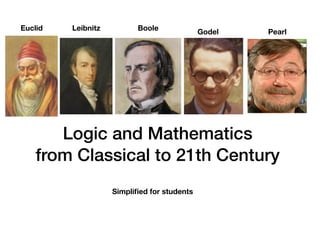
  • 1. Logic and Mathematics from Classical to 21th Century Euclid Leibnitz Godel Pearl Boole Simplified for students
  • 2. Contents Tools (WolframAlpha and Python) Classical Western Logic and Mathematics Non-Western Mathematics Rebirth of Western Mathematics Graphing Equations 20th and 21 Century Mathematics Logic, Sets, and Probability Causal Models and Reasoning Advanced Topics: Causal Reasoning and Deep Learning Continuous Probability Distributions This is mostly a basic presentation not requiring calculus A more advanced set of slides has been added at the end The simple topics in this presentation (e.g. logic,sets, probability, networks, algorithms number theory) would provide a more interesting math curriculuum than geometry, trigonometry, and algebraic manipulation.
  • 3. Tools Every student in high school should know WolframAlpha and Python. WolframAlpha to perform computations and Python to understand programming
  • 5. WolframAlpha Mathematics Elementary Math Algebra Calculus & Analysis Geometry Plotting & Graphics Differential Equations Numbers Trigonometry Linear Algebra Discrete Mathematics Number Theory Complex Analysis Applied Mathematics Logic & Set Theory Mathematical Definitions Continued Fractions Statistics Famous Math Problems Probability
  • 6. Python Programming Language Python is an easy to learn, powerful programming language. It has efficient high-level data structures and a simple but effective approach to object-oriented programming. Python’s elegant syntax and dynamic typing, together with its interpreted nature, make it an ideal language for scripting and rapid application development in many areas on most platforms. The Python interpreter and the extensive standard library are freely available in source or binary form for all major platforms from the Python Web site, https://www.python.org/, and may be freely distributed. The same site also contains distributions of and pointers to many free third party Python modules, programs and tools, and additional documentation. The Python interpreter is easily extended with new functions and data types implemented in C or C++ (or other languages callable from C). Python is also suitable as an extension language for customizable applications. This tutorial introduces the reader informally to the basic concepts and features of the Python language and system. It helps to have a Python interpreter handy for hands-on experience, but all examples are self-contained, so the tutorial can be read off-line as well. For a description of standard objects and modules, see The Python Standard Library. The Python Language Reference gives a more formal definition of the language. To write extensions in C or C++, read Extending and Embedding the Python Interpreter and Python/C API Reference Manual. There are also several books covering Python in depth. Tutorial Python is an easy to learn powerful programming language. There are many valuable libraries that provide much additional capabilities. The interpreter is an important tool for caatching errors.
  • 8. Classical Logic and Mathematics
  • 9. Aristotle’s Logic Aristotle All Dogs are Animals D -> A leonard is a Dog l is in D Conclusion Given leonard is a Animal l is in A Pictures Not Necessarily True: (Converse) All Animal are Dogs - (Inverse) Not a Dog means Not an Animal Always True: (Contrapositive) Not an Animal means Not a Dog Dogs Animals True: All Dogs are Animals Dogs Animals Not an Animal mean Not a Dog False: All Animals are Dogs cat Not a Dog means Not an Animal (cat is a Counterexample) Given: Guilty people always tell lies Test: Which sentence must be true? If he tell lies then he is guilty If he is not guilty he won’t tell lies If he is not telling lies then he is not guilty Given: Whatever doesn’t kill you makes you stronger Contrapositive is true: Whatever doesn’t make you stronger kills you What is wrong with this logic?
  • 10. Aquinas Proof of God’s Existence by St Thomas Aquinas St Thomas Aquinas was a follower of Aristotle in 1200 AD. He believed that the existence of God could be proved by logic rather than taken on faith. Below is the best of his 5 proofs. Proof from First Cause: (or what caused the Big Bang?) 1. In the world, we can see that things are caused. 2. But it is not possible for something to be the cause of itself because this would entail that it exists prior to itself, which is a contradiction. 3. If that by which it is caused is itself caused, then it too must have a cause. 4. But this cannot be an infinitely long chain, so, there must be a cause which is not itself caused by anything further. 5. This everyone understands to be God. Can you find a flaw in this logic? Mandala D C B A Which came first? Chicken or Egg? Wheel of Life Samsara
  • 11. Pathways to Knowledge Observation - This is the earliest pathway. The ancient civilizations studied the motion of the planets and could predict eclipses Theoretical - This pathway abstracts from observation and attempts to use logical or mathematical reasoning to understand the world. Aristotle’s work was based on observation and logic Experimental - This pathway explores the real world by initializing a system, controlling inputs, and measuring outputs. It is often based on a theoretical prediction. The combination of observation, theory, and experiment is the basis of the modern science Faith - This pathway believes in supernatural forces that explain everything. It dos not make predictions and can not be disproved by observation, theory, or experiment. Engineering - Combines focused theory, experiment, and design to create useful constructs. The Egyptian pyramid builders and the Romans were excellent engineers. Hero of Alexandria (50 AD) was a Greek who created a small steam engine. Unfortunately engineering advances most quickly in times of war. (planes, bombs) 20th Century Computational Science - Using computers to simulate systems 21th Century Big Data - Using computers to detect patterns in massive data sets
  • 12. Greek Mathematicians The four most famous Greek mathematicians are Euclid (400 BC), Pythagoras (500 BC), Diophantus (265 BC), and Archimedes (212 BC). Euclid invented geometric reasoning. Why are undefined terms like points necessary? Pythagoras proved a famous theorem, Diophantus described integer solutions to equations, and Archimedes calculated the area of the circle by approximations with triangles. a = 3 b = 4 c = 5 3^2 + 4^2 = 5^2 Undefined Terms Definitions Assumptions (Axioms) Theorems b b a a Circle Area = 𝛑* r^2 Triangle Area = 1/2 a*b Euclid Pythagoras Diophantus Archimedes Rectangle Area = a*b
  • 13. a a a a b b b b c c c c a b b a a a b b c c a a b b Pythagorean Theorem in Pictures 90 Triangle T Square 1 and Square 2 have the same sides (a + b) and thus the same area. Each square contains 4 copies of Triangle T. The area that is left when you take out the 4 copies of T must be equal. In Square 1, it is two squares with areas a^2 and b^2 with total area a^2 + b^2. In Square 2, it is 1 big square with area c^2. Since both areas are the same: a^2 + b^2 = c ^2 T T T T T T T T Square 1 Square 2 in Triangle T
  • 14. The Line (Euclid, Zeno, Plato) Euclid Euclidean Geometry: Line and point are undefined terms Assumption: Two points determine one line Assumption: Parallel lines never meet Non-Euclidean Geometry These assumptions seem obvious but they are not always true. On the earths surface, there are many north-south lines between the North and South Pole, all of them are heading in the same direction (south). Plato Plato taught that lines in the observed world are not truly straight or continuous . He believed that there was an “ideal line” that all the observed lines were imperfect copies. It sounds strange but this is not really a continuous line because all laptops are digital and use discrete pixels. Philosophers still argue whether humans discovered straight lines (and numbers) or invented them. Zeno One form of Zeno’s paradox 1 is the following question: How can a continuous line of length 1 be made up of points of length 0? This question was unsolved by mathematicians for over 2000 years. Even now there are issues in physics related to the meaning of points.
  • 15. Prime Numbers A prime number is an integer > 1 not divisible evenly by any smaller number except 1 Examples: 2, 3, 5, 7, 11, 13,17 are prime. 6 = 2 *3, 9 = 3*3, 30 = 2*3*5 and 12 = 2*2*3, are not. Every integer > 1 is either a prime or the product of primes (factors) Euclid Wolframalpha First 10 primes Eratosthenes Euclid proved that there are an infinite number of primes. Eratosthenes discovered a way to generate all the primes less than some number Wolframalpha Primes less than 1000 Wolframalpha Factor 90 There is no known fast way to factor very large numbers even with supercomputer This problem is very important for Internet security. It is hard to find very large primes even with supercomputers Primes have been studied for over 2000 years, but there are still many unanswered questions
  • 16. Factoring Numbers into Primes A prime number is an integer > 1 not divisible evenly by any smaller number except 1 Examples: 2, 3, 5, 7, 11, 13,17 are prime. 6 = 2 *3, 9 = 3*3, 30 = 2*3*5 and 12 = 2*2*3, are not. Every integer > 1 is either a prime or the product of primes (factors) Start with a list of primes in order. Example: 2, 3, 5, 7,11, 13,17,19, 23, 29 For any number N less than 29*29, it is possible to calculate the factors of N Start by checking to see if N can be divided evenly by 2 to give N/2. Keep dividing by 2 as much as possible Keep track of how many times you have divided by 2 Continue by checking to see if the result can be divided by 3. Keep dividing by 3 as much as possible Keep track of how many time you have divided by 3 Continue the same way through the list of primes. Stop if result =1 If result is not 1 then add it to the list of factors Example: Factor 84. 84/2 = 42, 42/2 = 21 (2,2). 21/3 = 7 (3), 5 doesn’t divide 7, 7/7 =1 (7). Result 84 = (2 * 2* 3 *7 ) Example: Factor 50. 50/2 = 25 (2). 3 doesn’t divide 25. 25/5 = 5, 5/5 = 1 (5,5) Result 50 =( 2* 5*5 ) Example: Factor 62. 62/2 = 31 (2). None of the other primes divide 31. Add 31 as a factor(31). Result = (2 * 31)
  • 17. Factoring Numbers into Primes Program Python Program for Factoring Output = [2, 2, 3, 7] def remainder (n, p): return (divmod (n,p)[1]) n = 84 factors = [] primelist = [2,3,5,7,11, 13,17,19,23,29] for p in primelist: while remainder (n,p) == 0: factors = factors + [p] n = n/p if n == 1: break if (n != 1): n = int(n) factors = factors + [n] print (factors) divmod is a built-in Python function divmod (n,p) = (quotient n/p, remainder) divmod(n,p)[0] = quotient n/p divmod(n,p)[1] = remainder from n/p Example: divmod(11, 2) = (5,1) Example: divmod (7, 3) = (2,1) Example: divmod (20, 5) = (4,0) Example: divmod ( 20, 7) = (2,6)
  • 18. Prime Numbers A prime number is an integer > 1 not divisible evenly by any smaller number except 1 Examples: 2, 3, 5, 7, 11, 13,17 are prime. 6 = 2 *3, 9 = 3*3, 30 = 2*3*5 and 12 = 2*2*3, are not. Every integer > 1 is either a prime or the product of primes (factors) Euclid proved that there is no largest prime ( same as proving the number of primes is infinite). Proof by contradiction from logic. Assume something is true and then prove that it is false Assume Earth is flat. Then if I travel in same direction, I never return to the starting point. Travel around the Earth and return to start. This proves that the Earth is not flat. Assume that L is the largest prime. Create a list of primes in order 2, 3, 5, 7, …., L Multiply all of the primes together and add 1 to get P = (2 *3*5**7 ………..*L) +1 Try to factor P. All of the primes on the list leave a remainder of 1 and can’t divide P Hence either P is a prime or is divisible by some prime not on the list. Therefore L can’t be the largest prime Example: if list is 2,3 then P =(2*3) +1 = 7 (2 and 3 leave remainder 1 when dividing 7) Example: If list is 2,3,5 then P = 2*3*5 = 30 +1 = 31 i (2,, 3, 5 leave remainder 1 when dividing 31) Example: If list is 2,3,5,7 then P= 2*3*5*7 = 210 +1 = 211 is a prime Example:If list is 2,3,5,7,11,13 then P +1 = 2*3*5*7*11*13 +1 = 30031 = 59 * 509 Euclid
  • 19. Finding Primes using Sieve of Eratosthenes Video of the Sieve of Eratosthenes Eratosthene Eratosthenes found a method for discovering all the primes below a given number N Let N = 30 as an example. Then the list of all numbers below N is 2,3,4,5,6,7,8,9,10,11,12,13,14,15,16,17,18,19,20,21,22,23,24,25,26,27,28,29,30 The smallest black number on the list is 2. It is a prime. Mark it in green 2,3,4,5,6,7,8,9,10,11,12,13,14,15,16,17,18,19,20,21,22,23,24,25,26,27,28,29,30 Find all the numbers that are divisible by 2 and mark them in red. They are not primes 2,3,4,5,6,7,8,9,10,11,12,13,14,15,16,17,18,19,20,21,22,23,24,25,26,27,28,29,30 The smallest black number on the list is 3. It is a prime. Mark it in green 2,3,4,5,6,7,8,9,10,11,12,13,14,15,16,17,18,19,20,21,22,23,24,25,26,27,28,29,30 Find all the numbers that are divisible by 3 and mark them in red. Some are already red. 2,3,4,5,6,7,8,9,10,11,12,13,14,15,16,17,18,19,20,21,22,23,24,25,26,27,28,29,30 The smallest black number the list is 5. It is a prime. Mark it in green 2,3,4,5,6,7,8,9,10,11,12,13,14,15,16,17,18,19,20,21,22,23,24,25,26,27,28,29,30 Find all the numbers that ar divisible by 5and mark them in red. Most are already red. 2,3,4,5,6,7,8,9,10,11,12,13,14,15,16,17,18,19,20,21,22,23,24,25,26,27,28,29,30 The smallest black number is 7. None of the remaining numbers in black are divisible by 7 Color them all green. 2,3,4,5,6,7,8,9,10,11,12,13,14,15,16,17,18,19,20,21,22,23,24,25,26,27,28,29,30 The primes are in green 2,3,5,7,11,13,17,19,23,29
  • 20. Python Program for the Sieve of Eratosthenes Video of the Sieve of Eratosthenes This program prints the primes up to 1000 using the Sieve of Eratosthenes Eratosthenes Output [2, 3, 5, 7, 11, 13, 17, 19, 23, 29, 31, 37, 41, 43, 47, 53, 59, 61, 67, 71, 73, 79, 83, 89, 97, 101, 103, 107, 109, 113, 127, 131, 137, 139, 149, 151, 157, 163, 167, 173, 179, 181, 191, 193, 197, 199, 211, 223, 227, 229, 233, 239, 241, 251, 257, 263, 269, 271, 277, 281, 283, 293, 307, 311, 313, 317, 331, 337, 347, 349, 353, 359, 367, 373, 379, 383, 389, 397, 401, 409, 419, 421, 431, 433, 439, 443, 449, 457, 461, 463, 467, 479, 487, 491, 499, 503, 509, 521, 523, 541, 547, 557, 563, 569, 571, 577, 587, 593, 599, 601, 607, 613, 617, 619, 631, 641, 643, 647, 653, 659, 661, 673, 677, 683, 691, 701, 709, 719, 727, 733, 739, 743, 751, 757, 761, 769, 773, 787, 797, 809, 811, 821, 823, 827, 829, 839, 853, 857, 859, 863, 877, 881, 883, 887, 907, 911, 919, 929, 937, 941, 947, 953, 967, 971, 977, 983, 991, 997] Wolframalpha Primes less than 1000 N = 1000 primeindex = [] for i in range (1, N): primeindex = primeindex + [1] numbers = [] for j in range (1, N - 1): numbers = numbers + [j + 1] index = 0 prime = numbers[index] primelist =[prime] while (index < N - 1): for k in range (index + prime, N - 1, prime): primeindex [k] = 0 m = index + 1 if (m < N -1): while primeindex [m] == 0: m = m + 1 if m == N - 1: break if m == N - 1: break index = m prime = numbers[index] primelist= primelist + [prime] print(primelist)
  • 21. Greatest Common Divisor using Primes A prime number is an integer > 1 not divisible evenly by any smaller number except 1 Examples: 2, 3, 5, 7, 11, 13,17 are prime. 6 = 2 *3, 9 = 3*3, 30 = 2*3*5 and 12 = 2*2*3, are not. Every integer > 1 is either a prime or the product of primes (factors) The greatest common divisor (gcd) of two integers is the largest integer that divides both Example : gcd (6,9) =3, gcd (12,30) = 6 , gcd (6,30) = 6 Wolframalpha for gcd(30, 12) In general, gcd = the product of prime factors found in both integers. Note that gcd (n, 0) = n To calculate the gcd (N. D) (greatest common divisor of two numbers N and D). Factor N into primes. Factor D into primes. Find the common primes that appear in both factors. gcd (N, M) is equal to the product of the common prime factors. Examples: gcd(6,9). 6=2*3 and 9 = 3*3 . Common factor is 3. Thus gcd(6,9) = 3 gcd (12,30) 12 = 2*2*3 and 30 = 2*3*5. Common factors are 2,3. Thus gcd(12,30) = 6` gcd (20,30) 20 = 2*2*5 and 30 = 2*3*5. Common factors are 2, 5. Thus gcd(20,30) = 10 The gcd is useful for simplifying fractions. Let g = gcd(N, D) The fraction N/D is equal to (N/g) / (D/g) Example 6/9 . 6/9 = (2*3)/(3*3) . The gcd is 3 and 6/9 = 2/3 Example 12/30. 12/30 = (2*2*3)/(2*3*5). The gcd is 2*3 =6 and 12/30 = 2/5 Example 20/30. 20/30 = (2*2*5)/(2*3*5) . The gcd is 2*5 =10 and 20/30 = 2/3 1/4 1/4 1/2 1/2 2/4 or Simplifying Fractions
  • 22. Greatest Common Divisor using Primes def remainder (n, p): return (divmod (n,p)[1]) n = 84 m = 98 commonfactors = [] primelist = [2,3,5,7,11, 13,17,19,23,29] for p in primelist: while remainder(n,p) == 0: n = n/p if remainder (n,p) == 0: m = m/p commonfactors = commonfactors + [p] if n == 1: break if n != 1: n = int(n) if remainder(m,n) == 0: commonfactors = commonfactors + [n] gcd = 1 for p in commonfactors: gcd = gcd * p print ("common factors =",commonfactors, "and gcd =", gcd) Python Program for gcd using Primes Output: common factors = [2,7] and gcd = 14
  • 23. Euclid’s Greatest Common Divisor Method For large integers, it is hard to find the prime factors. Euclid found a new way to compute gcd Let the 2 integers be called Large and Small with Large greater than or equal to Small. Divide Large/Small and keep Remainder. This is often written as Remainder = Large mod Small Examples 9/6 = 1 with Remainder 3 , 20/3 = 6 with Remainder 2, 30/5 = 6 with Remainder 0 Key ideas: gcd (Large, Small) = gcd (Small, Remainder). If Remainder = 0 then gcd = Small Examples gcd (9,6) = gcd (6,3) =gcd (3,0) =3 and gcd (17,6) = gcd (6, 5) = gcd (5,1) = gcd (1,0) =1 Why does gcd (Large, Small) = gcd (Small, Remainder)? Explanation: Large / Small = n with Remainder is the same as Large = n * Small + Remainder Let d = gcd (Large, Small) then Large/d =n * Small/d + Remainder/d Since d divides Large and Small, it must also divide the remainder. Euclid A prime number is an integer > 1 not divisible evenly by any smaller number except 1 Examples: 2, 3, 5, 7, 11, 13,17 are prime. 6 = 2 *3, 9 = 3*3, 30 = 2*3*5 and 12 = 2*2*3, are not. Every integer > 1 is either a prime or the product of primes (factors) The greatest common divisor (gcd) of two integers is the largest integer that divides both Example : gcd (6,9) =3, gcd (12,30) = 6 , gcd (6,30) = 6 In general, gcd = product of prime factors found in both integers. Exception gcd (n, 0) = n Using Wolframalpha for gcd(30, 12) Algorithm : Read 2 numbers a, b. If a> b then Large = a , Small = b else Large = b , Small = a Remainder = Large mod Small. Repeat until Remainder = 0. Large <- Small and Small <-Remainder. Remainder <- Large mod Small When Remainder = 0 then gcd = Small
  • 24. Python Program for Euclid’s GCD Method Sample Output for input 62 and 24 def remainder(n,p): return(divmod(n,p)[0]) def quotient (n,p): return (divmod (n,p) [1]) a= 62 b =24 print (" ") Large = max(a,b) Small = min(a,b) print("gcd(",Large, ",", Small,")") Remainder = remainder(Large, Small) Quotient = quotient(Large, Small) print ("Quotient =",Quotient,"Remainder=", Remainder) print(" ") while (Remainder >0) : Large = Small Small = Remainder print("gcd(",Large, ",", Small,")") Remainder = remainder(Large, Small) Quotient = quotient(Large, Small) print ("Quotient =",Quotient,"Remainder=", Remainder) print(" ") gcd = Small print ("gcd =", gcd) gcd( 62 , 24 ) Quotient = 2 Remainder= 14 gcd( 24 , 14 ) Quotient = 1 Remainder= 10 gcd( 14 , 10 ) Quotient = 1 Remainder= 4 gcd( 10 , 4 ) Quotient = 2 Remainder= 2 gcd( 4 , 2 ) Quotient = 2 Remainder= 0 gcd = 2
  • 25. Irrational Numbers Let x= Sqrt (2) or x*x = x^2 = 2. x can not be an integer. 1*1 = 1 (too small) and 2*2 =4 (too large) Proof by contradiction that x can’t be a fraction. Assume x is a fraction N/D. Factor N and D into primes. Example . N = p1 *p2 *p3 and D = p1 * p4 . x = (p1*p2*p3) /(p1 *p4) = (p2*p3)/(p4) Common prime factors can be eliminated by division to simplify N/D Since x is not an integer. D must contain a prime factor that is not in N Example: If N = 2*3*5 and D= 2 *3 * 7 then N/D = (2*3*5)/(2*3*7) = 5/7 If D did not have the factor 7, then N/D = (2*3*5)/(2*3) = 5/1 = 5 an integer Since x = N/D then x*x = 2 =( N/D) * (N/D) = (N*N)/(D*D) = N^2/D^2 The factor of N^2 are just the factors of N doubled. The same is true for D Example: If N = p1 *p2*p3 then N^2 = p1*p1*p2*p2*p3*p3 If N = 2 *3 the N^2 = (2*2)*(3*3) Since D contains a prime factor that is not in N, D^2 must contain a factor that is not in N^2 Thus simplifying the fraction x^2 = N^2/D^2 can not make the denominator 1 Hence x^2 can not be an integer and specifically can not be 2. Pythagoras Pythagoras believed that all numbers were fractions. He led a cult based on that belief. In legend, Hippasus proved that the Sqrt (2) was not a fraction (rational number) and was drowned by the gods in punishment. Hippasus (a/b) * (c/d) = (a *c)/(b*d) Example: 2/3 * 5/7 =10/21 Multiplying Fractions
  • 26. Diophantine Equations Diophantus Diophantine Equations are equations where solutions are restricted to integers . Example: 2 * x = 1 can’t be solved. Also 2 * x + 4 * y= 3 can’t be solved because 2 divides the left side of the equation evenly but not the right side. A simple example that always has solutions is p1 * x - p2 * y = r where p1 and p2 are primes and r can be any integer Simple: Example: 5 * x - 7 *y =1 or 5x -7y = 1. Here’s how to solve it: Add 7y to both sides of the equation to get 5x = 1 + 7y Start with y = 0 and 1 +7y =1 Try to solve 5x =1. 5 doesn’t divide 1 evenly Make y = 1 and then 1+ 7y = 8. Try to solve 5x = 8. 5 doesn’t divide 8 evenly Make y = 2 and then 1 + 7 *2= 15. Try to solve 5x=15. This works x = 3 if y = 2. A solution is x=3 and y=2. Check 5 *3 - 7 *2 = 1 This method works for any two primes p1 and p2 Another simple example is 7x -11y = 2 . Adding 11y to both sides gives 7x = 2 + 11y Start with y = 0 and 2 + 11y = 2. Try to solve 7x = 2. 7 doesn’t divide 2 evenly. Make y = 1 and 2 + 11y =2 + 11= 13. Try to solve 7x = 13. 7 doesn’t divide 13 evenly Make y = 2 and 2 + 11y= 2 +22 =24. Try to solve 7x = 24 . 7 doesn’t divide 24 evenly Make y = 3 and 2 + 11y = 2 + 33 =35 Try to solve 7x = 35. This works x= 5 if y = 3 A solution is x = 5 and y = 3. Check 7 * 5 - 11 *3 = 2
  • 27. Diophantus def remainder (n,p): return(divmod (n,p)[1]) def quotient (n,p): return(divmod (n,p)[0]) p1 = 23 p2 = 47 r0 = 2 r = r0 y = 0 #Solve p1 * x - p2 ^ y = r0 (Comment) while remainder (r,p1) != 0: y = y + 1 r = r + p2 x = quotient(r,p1) print ("x =", x) print ("y =",y) print (p1 ,"*" ,x ,"-", p2, "*", y, "=", p1 *x - p2*y) The Output is: x= 43 y= 21 23 * 43 - 47 * 21 = 2 Python Program for Simple Diophantine Equation Solving p1 * x - p2 *y = r
  • 28. Diophantus Famous Diophantine Equations From Pythagoras: In the right triangle below What are the integer solutions? Example a = 3, b = 4 , c = 5 3^2 + 4^2 = 9 + 16 = 25 = 5^2 There are infinite many solutions of the form a = t^2 -1 , b =2*t, c = t^2 +1 for any integer t >0 because (t^2 -1 )^2 + (2*t)^2 = (t^2 + 1) ^2 If t =2 then a = 2^2 -1 = 3, b= 2*2 =4, and c=2 ^2 +1 = 5 If t =3 then a= 3^2 -1 = 8 , b = 2*3 = 6 and c = 3^2 +1 =10 Check 8^2 +6^2 = 64 +36 = 100 = 10^2 From Fermat (1665): has no solution for x and y > 0 and n > 2 Fermat claimed to have a proof but no one could find one for over 300 years until Andrew Wiles (with Richard Taylor) proved that there were no solutions in 1995
  • 29. Bonus: Chinese Remainder Theorem Modular arithmetic: When integer N is divided by an integer p the result is an integer q + a remainder r. Examples: 13/5 = 2 + remainder 3. 20/3 = 6 + remainder 2. 5/7 = 0 with remainder 5. The remainder is sometimes written as N mod d. Examples 13 mod 5 = 3. 20 mod 3 = 2 Doing N mod 12 is sometimes called clock arithmetic. If it is 5 PM what is the time in 9 hours. 5 + 9 = 14. 14 mod 12 = 2. Time is 2 AM. The Chinese Remainder Theorem solves the problem Find N given that N mod p1 = r1 and N mod p2 = r2. In other words , find N if N/p1 has reminder r1 and N/p2 has remainder r2 The solution can be easily found if p1 and p2 are primes using Diophantine equations Find x and y such that p1 * x - p2 * y =1 Then N = r2 * p1 *x - r1 *p2*y . Example: We solved the equation 5x-7y=1 on the slide on Diophantine Equations The solution is x = 3 and y =2 . Check 5 *3 - 7*2 = 1 To solve N mod 5 = 2 and N mod 7 = 3. N = 3*5*3 - 2 * 7*2 = 45 -28 = 17 Check 17/5 = 3 + remainder 2 and 17/7 = 2 + remainder 3. Thus 17 mod 5 = 2 and 17 mod 7 = 3 This method was discovered by the Chinese mathematician Sun Tzu around 200 AD. It is added because it follows easily from s Diophantine equation Clue to why this works: (p1 * x) mod p2 =1 and (p2 *y) = -1 mod p1 Sun Tzu
  • 30. Secret Code with Chinese Remainder Theorem A B C D E F G H I J K L M N O P Q R S T U V W X Y Z 1 2 3 4 5 6 7 8 9 10 11 12 13 13 13 16 17 18 19 20 21 22 23 24 25 26 Choose 2 primes: for example 5 and 7 To code a letter, look at the corresponding number N Calculate N mod 5 and N mod 7, (Remainders when dividing N by 5 and 7 For example: to code Q. Find 17 mod 5 = 2 and 17 mod 7 = 3 The code for Q is (2,3). Only someone knowing the primes and the Chinese Remainder Theorem can decode the message The code for Kaya is: Coding K 11 mod 5 = 1 and 11 mod 7 = 4 (1,4) Coding A 1 mod 5 =1 and 1 mod 7 = 1 (1,1) Coding Y 25 mod 5 =0 and 25 mod 7 = 4 (0,4) Coding A 1 mod 5 =1 and 1 mod 7 = 1 (1,1) Kaya becomes (1,4), (1,1), (0,4) , (1,1) To decode (r1, r2) solve N mod 5 = r1 and N mod 7 = r2 Solution is N = r2 * 3 * 5 - r1 * 2*7. If N is less than 1 or greater than 26, it is possible to add or subtract 35 This is still a solution since 35 mod 5 = 0 and 35 mod 7 = 0 For example (1,4) gives N = 4*3*5 - 1*2*7 = 60 -14 = 46. Then 46 -35 = 11 (Letter = K)
  • 31. Python Program for Chinese Remainder Theorem def remainder (n,p): return (divmod (n,p) [1]) def quotient (n,p): return (divmod (n,p) [0]) p1 = 5 p2 = 7 Nmodp1 = 1 Nmodp2 = 4 r0 = 1 r= r0 y = 0 #Solve p1 * x - p2 ^ y = r (Comment) while remainder (r,p1)!= 0: y = y + 1 r = r + p2 x = quotient(r,p1) print ("x =", x) print ("y =",y) print (p1 ,"*" ,x ,"-", p2, "*", y, "=", p1 *x - p2*y) N = Nmodp2 * p1 * x - Nmodp1 * p2 *y while N >= (p1 * p2): N = N - (p1 *p2) while N < 0: N = N + (p1 * p2) print ("N =", N) Output is x = 3 y = 2 5 * 3 - 7 * 2 = 1 N = 11 Sun Tzu
  • 32. Famous Unsolved Problems with Prime Numbers Twin Primes: Twin primes are two primes whose difference is 2. Examples include (3,5) (5, 7) (11,13) (17, 19), (29,31)(41,43) (59,61) (71, 73) Primes less than 80: 2, 3, 5, 7, 11, 13, 17, 19, 23, 29, 31, 37, 41, 43, 47, 53, 59, 61, 67, 71, 73, 79 Are there an infinite number of twin primes? No one knows. Goldbachs’s Conjecture: Every even number (divisible by 2) greater than 2 is the sum of two primes Every even number tested so far is the sum of two primes. No one knows if this is always true. primelist = [2, 3, 5, 7, 11, 13, 17, 19, 23) for i in range (2,16): even = 2 * i for p in primelist: q = even - p if primelist.count (q) != 0: print ( even, "=", p, "+" , q) break Python program to check Goldbach’s Conjecture up to 30 4 = 2 + 2 6 = 3 + 3 8 = 3 + 5 10 = 3 + 7 12 = 5 + 7 14 = 3 + 11 16 = 3 + 13 18 = 5 + 13 20 = 3 + 17 22 = 3 + 19 24 = 5 + 19 26 = 3 + 23 28 = 5 + 23 30 = 7 + 23 Output Can you check Goldbach’s conjecture for 80?
  • 33. Roman Numerals Highest number used was MMMCMXCIX = 3999 but MMMCMDXCLIXVIII = 4557 Roman Numeral Converter Higher numbers: Line above multiples by 1000 . V = 5000 Box around multiplies by 100,000. V = 500,000 Addition and Multiplication are very difficult using Roman numerals What is IX * VII? Romans used abacuses
  • 34. Converting Roman Numerals to Base 10 Numbers The basic rules are simple for a correct Roman number. If a numeral’s value is less than its successor’s than subtract its value from the total else add its value to the total rnumber = "MMMCMXLIX" l = len(rnumber) result = 0 for i in range (0, l - 1): print (rnumber[i]) numeral =rnumber [i] n = value(numeral) successor = rnumber[i + 1] s= value(successor) if s > n: result = result - n else: result = result + n last = value (rnumber [l -1]) result = result + last print(result) def value (numeral): if numeral == "I": return (1) if numeral == "V": return (5) if numeral =="X": return (10) if numeral == "L": return (50) if numeral =="C": return (100) if numeral == "D": return (500) if numeral =="M": return (1000) return(0) Output = 3949 This program will give the correct output for legal Roma numbersand an output even for incorrect Roman numbers. The rules for correctness are complicated. The trick is to use the program on the next sllde to check the output by changing the output back to Roman numbers and comparing the result with the original. If they disagree the input was not a correct Roman number. Python Program
  • 35. Converting Base 10 Numbers to Roman Numerals The rules for this conversion are simple for numbers less than 4000. The conversion works correctly as long as the input is a number. It can be used to check conversions from Roman numbers to base 10 numbers. Roman input -> Base 10 -> Roman output. If Roman input doesn’t equal Roman output than Roman input has an error. def quotient(n, d): return (divmod(n,d)[0]) def remainder(n,d): return (divmod(n,d)[1]) n = 3949 rnumber = "" Ms = quotient (n , 1000) r = remainder(n, 1000) if Ms != 0: for i in range (1,Ms +1): rnumber = rnumber + "M" n = n - 1000 * Ms if r >= 400: if r >= 900: rnumber = rnumber +"CM" n = n - 900 elif r >= 500: rnumber = rnumber +"D" n = n- 500 else: rnumber = rnumber + "CD" n = n - 400 Python Program Cs = quotient (n , 100) r = remainder(n, 100) if Cs != 0: for i in range(1,Cs +1): rnumber = rnumber + "M" n = n - 100 * Cs if r >= 40: if r >= 90: rnumber = rnumber +"XC" n = n - 90 elif r >= 50: rnumber = rnumber +"L" n = n- 50 else: rnumber = rnumber + "XL" n = n - 40 Xs = quotient (n , 10) r = remainder(n, 10) if Xs != 0: for i in range (1,Xs +1): rnumber = rnumber + "X" n = n - 10 * Xs if r >= 4: if r >= 9: rnumber = rnumber +"IX" n = n - 9 elif r >= 5: rnumber = rnumber +"V" n = n- 5 else: rnumber = rnumber + "IV" n = n - 4 Is= n if Is != 0: for i in range( 1,Is +1): rnumber = rnumber + "I" n = n -Is print (rnumber) Output = MMMCMXLIX
  • 36. Bonus: Egyptian Mathematical Game From Math Playground Math Playground has many more games for all levels Egyptian Game: Mancala Can you beat computer?
  • 37. Non-Western Logic and Mathematics
  • 38. Ancient Chinese Mathematics and Science Hua Tuo Sun Tzu Zhang Heng Ten Computational Canons History of Chinese Science 4 Great Inventions: gunpowder, paper, printing, compass Shen Kuo Su Song Zu Chongzhi Chinese Mathematicians Chinese Mathematics Zhu Shijie History of Chinese Mathematics 10 Chinese Inventions Zhang Heng (100 AD) invented the seismoscope. Hua Tuo (170 AD) was the first surgeon to use general anesthesia. Liu Hui (250 AD) wrote a famous textbook on the Mathematical Art. Sun Tzu (350 AD) wrote the most famous Chinese mathematics book. Zu Chongzhi (450 AD) calculated Pi very accurately.Su Song (1050 AD) built a giant clocktower. Shen Kuo (1060 AD) invented the compass. Zhu Shijie (1303 AD) wrote an important algebra book. Liu Hui 
  • 39. z Indian Mathematicians Brahmagupta 650 AD Ramanujan 1910 Varadhan 1990 Aryabhata 500 AD and Scientists Raman 1930 Chandrashekar 1960
  • 40. z Islamic Mathematics Omar Khayyam 1100 Ibrahim Ibn Sinan 940 Sharaf al-Dīn 1200 Abu al-Assam 1000 AD
  • 42. z Rise of New Mathematics (1600 -1800) Descartes 1630 Fibonacci 1200 Pascal 1650 Fermat 1635 Euler 1740 Leibnitz 1670 Newton 1665 Bernoulli 1740
  • 43. z Fibonacci Sequence Fibonacci Fibonacci discovered a sequence of numbers with interesting properties and applications. The sequence starts with 0 and 1 and continues by adding the last 2 term to get the next term. See the steps below 0,1 next term is 0 +1 = 1 0,1,1 next term is 1 +1 = 2 0,1,1,2 next term is 1 + 2 = 3 0,1,1,2,3 next term is 2 + 3 = 5 0,1,1,2,3,5 next term is 3 + 5 = 8 0,1,1,2,3,5,8 next term is 5 + 8 = 13 fib =[0,1] n =20 for i in range(1,n): fib = fib + [fib[i-1] + fib[i]] print(fib) Python Program for first 21 terms Output [0, 1, 1, 2, 3, 5, 8, 13, 21, 34, 55, 89,144, 233, 377, 610, 987, 1597, 2584, 4181, 6765] Wolframalpha “First 20 Fibonacci Numbers” Surprisingly there is a formula for the nth Fibonacci number F(o) = 0 ( ( ) )
  • 44. z Decimal System (Base 10) The decimal system uses a positional structure based on digits 0,1,2,3,4,5,6,7,8,9 and powers of 10 to represent real numbers. Example 235= 2*10^2 +3^10 +5 *1 Parts of the system originated in China aand India and was transmitted to Europe through the Muslim world. Fibonacci introduced the decimal system to Italy from where it spread through Europe. Calculations are much easier using decimal notation than earlier systems (e.g. Roman numerals) Fractions can also be written using decimal notation. Recall that 10 ^ -n = 1/(10^n) Example 3/10 = .3 and 1/4 = 25/100 =2/10 + 5/100 = .25 (25 cents = 1/4 of 1 dollar) Fractions whose denominators are products of powers of 2 and 5 transform into finite decimals. Suprisingly all fractions transform into decimals that eventually repeat. To convert a repeating decimal to a fraction: Examples: Let x= .abababab… then 100 *x =ab.ababab….. 100 *x - x = 99 *x = ab.abab… - .ababab = ab. x =ab/99 Let y = .cdababab…. the y = cd/100 + .00abababab = ab/99 * 1/100 To convert a fraction n/d to a repeating decimal: By long division d n In each step there will be a remainder less than d. Sooner or later possibly after d steps there will be a repeated remainder that will start the repeating decimal.
  • 45. New Numbers As mathematicians tried to solve equations they had to invent new numbers. Everyone knew whole numbers (1,2,3,4,…..) from counting but these couldn’t solve all equations. To solve 2 * x = 1 they had to invent fractions x = 1/2 To solve x + 3 = 3, they had to invent zero x = 0 To solve x + 5 = 2, they had to invent negative numbers x = -3 To solve x ^ 2 = 2 they had to invent irrational numbers x = sqrt (2) (not a fraction) To solve x^2 = -1 they had to invent imaginary numbers x = sqrt (-1) = i (Philosophers argue whether these numbers are invented or already existed and then discovered) To simplify arithmetic, accountants and mathematicians adopted the base 10 system. Fractions can be be written as decimals. Examples (3/10 = .3) (67/100 = .67) (4/5 = .8) (3/4 =.75) Some fractions require infinitely long repeating decimals (1/3 =.33…) (1/6 = .166…) (7/99 =.0707…) Most decimals don’t end or repeat (irrational numbers. Example sqrt(2) = 1.41421356237….. The most famous equation and solution is the quadratic equation with solutions Note that because of the square root, the solutions could be irrational or imaginary. Using WolframAlpha at https://www.wolframalpha.com, it is possible to solve any quadratic by choosing a, b,c . For example if x^2 - 6*x + 5 = 0 then (a=1. b=-5, c = 6) The means one solution with + and another with - Solutions are x = 1 and x = 5 from formula on WolframAlpha
  • 46. Euler Paths 3 2 5 4 7 6 1 Euler Walk across every bridge once In general, on this walk every time you enter an island on a bridge, you must leave on a different bridge. To avoid getting trapped, there must be an even number of bridges on an island. There are two exceptions: the starting and ending islands. No solution. Too many odd islands 3 3 3 5 Removing a bridge Start on an island with odd number of bridges. Keep going and you will cross every bridge once and end on the other odd island 3 3 2 4 c a b e d f
  • 47. Euler and Hamiltonian Paths E I F D K G H C B A J Cross every Bridge once. Where should you start? Where will you end? Hamiltonian Paths: A related problem is to visit every island exactly once. This seems easier but no one knows the best method for solving this problem
  • 48. Euler Invariant For every connected network in the plane, the sum of Points + Regions - Edges = 2 (counting the outside region) This network has 11 Points, 18 Edges, 9 Regions and 11 + 9 - 18 = 2 Why does this formula work? Start with a point 1 9 8 7 6 5 4 3 2 then there is 1 point , 0 edges and 1 region. Thus 1 -0 +1 = 2 If you add a point, you must add an edge then the sum stays the same 3 points - 2 edges +1 region = 2 To create a new enclosed region, you must add an edge then the sum stays the same 3 points - 3 edges + 2 regions = 2
  • 49. z Counting Trees A tree is a connected network with no loops. N points, N -1 edges and 1 region Two trees are equivalent if they have the same shape There is only 1 tree with 2 points There is only 1 tree with 3 points There are 2 trees with 4 points There are 3 trees with 5 points How many trees are there with 6 points?
  • 50. z Counting Trees (cont) With 6 points and 5 edges, it is possible to form 6 trees with different shapes. Note that some trees may look different but have the same shape after transformations For example is the same as
  • 52. z Graphing Equations Graphing combines algebra and geometry One of the most important advance in mathematics Unified much of previous mathematics Invented in 1600’s by Descartes Descartes also revolutionized philosophy “I think therefore I am” is the basis of his view of reality Descartes
  • 53. z Graphing Points Basic idea: consider 2 unknowns: x and y Put x on a number line (x axis) from left to right Put y on a number line(y axis) from bottom to top Number lines meet at x=0 and y=0 Let x = 2 and y= 3 for example Plot (point x = 2 and y = 3 ) “Plot” is another word for graphing x=2 and y=3 or (2,3) Plotting can be done on https://www.wolframalpha.com/ x axis y axis
  • 54. z Graphing Points Plot point x=-2 and y = 4 (-2, 4) Note both number lines (axis) goes from negative to positives This is only a partial pictures Plotting can be done on https://www.wolframalpha.com/ x axis y axis ____________ | | x = -2 and y=4 (-2, 4)
  • 55. z Graphing Points Plot point (-3, -1) or x=-3 and y =- 1 Plotting can be done on https://www.wolframalpha.com/ x axis y axis (-3, -1)
  • 56. z Graphing Lines Key idea : An equation in two variables (x,y) can give many points to plot For example : x + y = 6 gives x =0, y= 6 or (0,6) and (1,5), (2,4), (3,3),(4,2), (5,1), (6,0) and also (7, -1), (-2, 8) and many more including fractions like x = 2 1/2 and y = 3 1/2 (2.5, 3.5). Decimals $2.50 + $3.50 = $6 Putting them all together on a graph gives the straight line below Plot x +y = 6 Plotting can be done on https://www.wolframalpha.com/ x axis y axis (0,6) (6,0) (3,3) (-1,7) (5,1) (1,5)
  • 57. z Graphing Two Lines Plotting can be done on https://www.wolframalpha.com/ It is possible to graph two equations at the same time. The points where the graphs intersect are solutions to the equations You can solve equations by algebra or geometry For example, Plot x + y =10 and x - y = 4 The two lines intersect at x=7 and y =3 (7,3) Note that the picture below starts at x=6 and y=2
  • 58. z Graphing Applied Equations Plotting can be done on https://www.wolframalpha.com/ d axis Distance = Speed * Time or d=s*t If you run at s = 5ft/sec for t = 4 sec, your distance traveled = 20 ft If your speed is always 5ft/sec then d = 5 * t This can be plotted as a straight line t axis
  • 59. z Graphing with Variables Squared Plotting can be done on https://www.wolframalpha.com/ x axis y axis The equation x^2 =y has a square It can be graphed but is not a line (called parabola) Some points are x= 0, y =0 (0,0) and x =2, y =4 (2,4) also (1,1),(3,9), (4, 16) Also x = -2 and y =4 (-2,4) since -2 * -2 = 4 and (-1,1),(-3,9),(-4,16) Plot y = x^2
  • 60. z Bonus: Useful Equation for Velocity (Gravity) nObjects fall down from gravity with distance = 16*time^2 or d= 16t^2 If you jump off a building 2000 ft high after 1 sec , you fall 16 *1 =16 ft, after 2 sec you fall 16 *4= 64 ft Faster after 3 sec you fall 16 *9 =144 ft after 10 sec you fall 16 *100 =1,600 ft. Plotting d= 2000 - 16 * t^2 Objects fall with distance = 16 * t^2 To find the average velocity between time t1 and t2, calculate the change in distance over the change in time (16 * t2 ^2 - 16* t1^2)/ (t2 -t1) Example: the average velocity between t1 = 2 and t2 = 3 is (16 *3^2 - 16 * 2^2) /(3-2) = 16 * 9 - 16 * 4 = 144 -64 = 80 ft /sec To approximate the velocity at time t1, calculate the average velocity between t1 and t1 + tsmall where tsmall is small For example, an approximate velocity at t = 3 with tsmall=.01 (16* 3.01^2 - 16 * 3^2) /(3.01 - 3) = (144.9616- 144) /.1= .9616/.1 = 96.16 This approximate velocity gets closer to the actually velocity as tsmall gets closer to 0. Isaac Newton invented calculus to find the limit.
 For gravity, thevelocity = 32 *t When t = 3 the velocity is 32*3 = 96
  • 61. z Useful Equation with Squares (Gravity) Plotting can be done on https://www.wolframalpha.com/ t axis d axis Objects fall down from gravity with distance = 16*time^2 or d= 16t^2 if you start on the ground and throw a ball with speed = s then the distance would d = s * t without gravity. With gravity it becomes d = s *t - 16 * t^2 Throw ball up with speed 80 ft per second, d = 80 *t - 16*t^2 = 80t-16t^2 Plotting this shows how high the ball will go and when it hits the ground
  • 62. z Graphing with Variables Squared Plotting can be done on https://www.wolframalpha.com/ x axis y axis The equations y = x^2 (parabola) and y = x (line) can be graphed Plot y = x^2 and y = x The parabola and the line meet in two points x = 0, y = 0 (0,0) and x=1, y=1 (1,1)
  • 63. z Graphing with Variables Squared Plotting can be done on https://www.wolframalpha.com/ x axis y axis The equation x^2 + y^2 =25 x = 3 and y = 4 (3,4) Check 3^2 + 4^2 9 + 16 =25 x = 0 and y = 5 (0,5) Check 0^2 + 5^2 =25 Plot x^2 + y^2 = 25. Result is a circle (3,4) (0,5)
  • 64. z Graphing with Cubic Powers Plotting can be done on https://www.wolframalpha.com/ x axis y axis Plot x^3 - x +2 =y gives a curve that has two bends Plotting y=2 gives a straight line The intersection of the line with the curve give three points (-1, 2), (0,2) and (1,2 Check x=1 and y=2 : Substitute in x^3 - x +2 =y gives 1^3 -1 +2 = 1-1 +2 = 2 (-1,2) (0,2) (+1,2)
  • 65. z Graphing with Three Variables Plotting can be done on https://www.wolframalpha.com/ It is possible to graph equations with three variables x,y,z For example, plot x^2 +y^2 +z^2 =9 Some solutions are (0,0,3) (1,2,2), (-2,-2, +1)
  • 67. Linear Algebra The Scalar Product ( ) of two vectors of the same dimension is the sum of the products of corresponding components. For example: (u1, u2, u3) (v1, v2,v3) = u1 *v1 + u2* v2 + u3 * v3 Example (4,1, 2) (2, -3,5) = 8 -3 + 10 =15 A Vector is a sequence of numbers. Example is v = (2,-3,5) The size of the sequence is the dimension of the vector .Dimension(v) =3 Two vectors of the same size can be added termwise Example is (2, -3, 5) + (4,1, 2) = (6,-2,7) A vector can be multiplied term-wise by an ordinary number(called a scalar) Example is 4 * (2, -3, 5) = (8, -12, 20) Vectors can be represented graphically. For example (1,2) beomes 0 1 2 2 1 (1,2) Length of a vactor v = sqrt (v v). Example length (1,2) = sqrt (1*1 + 2*2) = sqrt(5)
  • 68. Linear Algebra A Matrix is a 2 dimensional rectangular collection of numbers. For example M = ( 1 3 4) is a 2 by 3 matrix (2 0 5) An “n by k” matrix can multiply a “k by 1” matrix to give an “n by 1” matrix Note that a m by 1 matrix is just a sequence of numbers i.e. a vector For example: (1 3 4) (1) (1 *1 + 3*2 + 4*3) (19) (2 0 5) * (2) = (2 *1 + 0 *2 +5 *3) = (17) (3) In general, an “n by k” matrix A can multiply a “k by m” matrix B to give an “n by m” matrix C The (i,j)th term in C is the scalar product of the i row of A and the j column of B. For example, let A= [[1,2, 3], [2,0,5]] and B = [[4, 1],[5, 2] ,[6,3]] then C= A*B = [ [(1. 2,3) (4,5,6), (1,2,3) (1,2,3)][(2,0, 5) (4,5,6), (2,0,5) (1,2,3)]] C = [[32, 14)], [38,17]). See the tabular representation below. = C B A . =
  • 69. Matrix Multiplication def scalar(u, v): sum = 0 for i in range (0, len(u)): sum = sum + u[i] * v[i] return(sum) def row (i, matrix): r= matrix [i] return (r) def column(j, matrix): c=[] for i in range(0, len (matrix)): c = c + [matrix[i][j]] return(c) def matmult (mat1,mat2): mat3 =[] for i in range (0, len (mat1)): mat3row = [] for j in range (0, len (mat2[1])): s= scalar (row (i,mat1), column(j, mat2)) mat3row = mat3row + [s] mat3 = mat3 + [mat3row] return (mat3) m1 = [[1,2, 3], [2,0,5]] m2 = [[4, 1],[5, 2] ,[6,3]] m3 = matmult (m1, m2) print (m3) Python Output = [[32, 14], [38, 17]] WolframAlpha Additional analysis
  • 70. Geometric Algebra Comparison of Geometric and Vector Algebra Hestenes Another example (2*e1 + 3 * e2) * (4 * e1 + 5 * e2) = (2*4 +3 *5 + 0) + (2 *5 *e1 ∧ e2) - (3 *4 e1 ∧ e2) = 23 - 2 * e1 ∧ e2 Example: Let e1 and e2 be 2 vectors such that e1 e2 = 0 Then e1 * e2 = 0 + e1 ^ e2= e1^ e2. This is not a vector. Geometrically it is the 2 dimensional parallelogram generated by e1 and e2. The anti-symmetry gives an orientation tothe parallelogram Geometric Algebra is a system for doing linear algebra that provides many useful features and perspectives. It has a long history but had strong 20th century revival from David Hestenes The basic idea is to define a new vector product u * v Split u*v into symmetric and anti-symmetric parts u*v = 1/2 (uv +vu) +1/2 (uv-vu) When u and v are switched, symmetric part stays the same and anti- symmetric part reverses sign . The symmetric part is chosen to be u v. The anti-symmetic is written u ∧ v = - u ∧ v and called the wedge product Quarternions and Geometric Algebra
  • 71. 20th and 21th Century Mathematics
  • 72. Famous Mathematicians of the 20th Century The 20th Century was a golden age for mathematics inspired by physics, biology, and computer science. David Hilbert (German) presented 23 unsolved problems to mathematicians in 1900 that inspired much research. Henri Poincare (France) discovered much new mathematics including Chaos Theory. John von Neumann was one of the greatest mathematicians of all time. He invented Game Theory, Computer Architecture, and worked on the atom bomb. Kurt Godel solved one of Hilbert’s problems by showing that it was not possible to prove every true mathematical statement (Incompleteness Theorem). Andrew Wiles proved the most famous unsolved problem in mathematics called Fermat’s Last Theorem (there is no solution in integers for x,y,z in x^n + y^n = z^n if n >= 3. Shannon discovered Information Theory. Conway invented the Game of Life. Hilbert Poincare Von Neumann Godel Wiles Conway Shannon
  • 73. Collatz Conjecture In 1937, Lothar Collatz made the following conjecture: Start with any number N. If N is even divide it by 2 (N/2) or if if N is odd multiply it by 3 and add 1 (3*N + 1). Continue this procedure and eventually the result equals 1 and then repeats 1,4,2,1 This conjecture is satisfied by every number that been checked but no one knows if it is true for all numbers. An example is below. def remainder (N, d): return divmod(N, d) [1] def quotient (N, d): return divmod (N,d) [0] N = 7 while (N != 1): print(N) if remainder (N,2)== 0: N = quotient(N,2) else: N = 3 * N + 1 print(1) Python Program 7 22 11 34 17 52 26 13 40 20 10 5 16 8 4 2 1 Output 3 * 7 + 1 = 22/2 =
  • 74. Coloring Networks with 4 Colors Map makers discovered that they could color maps with only 4 colors such tha no two bordering states or countries had the same color. they asked if this was always true. It took 100 years and powerful computers for Haken and Appel prove it was. The map can be represented as a network where each point is a country and each edge is a border. Here are 4 countries that all border on each other. It is impossible for 5 countries to border on each other Haken+Appel
  • 75. Bonus: Ramsey Number Take one of the people P, she has edges going to the 5 others. At least 3 of the edges must have the same colors since there are only two colors. Say it is green going to P’s friends A,B,C. If any two of these friends know each , there is a green edge between them that will form a green triangle. If none of them know each other, then there is a triangle with all red edges and points A, B C. Frank Ramsey There are 6 people at a party. It is always true that there are 3 people who all know each other or 3 people who all don’t know each other. Form a network where the people are points, draw an edge between every two points with color green if the people know each other and red if they don’t. P A B C This problem can be generalized to how many people have to be at a party in order to have n people who all know each other or n people who all don’t know each other. The answer is known to be 18 for n = 4 but is not known for any higher n.
  • 76. Bonus: Shortest Distance in a Network 3 7 5 Start Finish 6 2 3 2 2 7 3 7 5 Start Finish 6 2 3 2 2 7 Begin at Start. At each step find the circle that is closest to Start among the circles with no distance entered. Enter the distance to Start into the circle. Continue these steps until you reach the Finish. See the example below. This algorithm was discovered by Edsger Dijkstra. 2 5 2 5 7 0 0 3 7 5 Start Finish 6 2 3 2 2 7 2 0 Edsger Dijkstra
  • 77. Shortest Distance in a Network (cont) 3 7 5 Start Finish 6 2 3 2 2 7 3 7 5 Start Finish 6 2 3 2 2 7 Continuing the example from the last slide. We find the Finish is 13 from the Start. 0 0 2 2 5 2 8 7 7 5 3 7 5 Start Finish 6 2 3 2 2 7 0 2 5 8 7 13 Edsger Dijkstra
  • 78. Bonus: Shortest Path 3 7 5 Start Finish 6 2 3 2 2 7 0 2 5 8 7 13 To find the shortest path given the shortest distance, work backwards from the Finish and use subtraction to find the path that was used to get thee shortest distance. For example, the first edge is between the node with 8 and the Finish since 13 - 5 = 8 while 13 - 7 does not equal 7 3 7 5 Start Finish 6 2 3 2 2 7 0 2 5 8 7 13 Here is the total shortest path This method for finding the shortest distance and path between any two circles is very quick. Surprisingly the problem of finding the shortest path that visits all of the circles (Traveling Salesman problem) is much more difficult. No one knows the best algorithm. Edsger Dijkstra
  • 79. Bonus: Minimum Spanning Tree in Network 1 7 5 6 2 3 2 2 7 Assume that the circles in the network are cities. Find the shortest collection of roads that will connect all the cities. The solution will have no loops (tree) since one of the roads is unnecessary The solution is to select at each step the smallest edge that can be added without forming a loop. Any choice when there is a tie. Stop when all circles are connected 1 7 5 6 2 3 2 2 7 1 7 5 6 2 3 2 2 7
  • 80. Bonus: Minimum Spanning Tree in Network (cont) 1 7 5 6 2 3 2 2 7 Assume that the circles in the network are cities. Find the shortest collection of roads that will connect all the cities. The solution will have no loops (tree) since one of the roads is unnecessary The solution is to select at each step the smallest edge that can be added without forming a loop. Any choice when there is a tie. Stop when all circles are connected 1 7 5 6 2 3 2 2 7 1 7 5 6 2 3 2 2 7 Can’t choose final length 2 edge because it will create a loop. Must choose length 3 edge Solution: Minimal length is 2 + 3 + 2 + 1 +5 = 13
  • 81. Bonus: Steiner Tree Problem The Steiner Tree problem is to find the shortest set of edges within a network that will link a collection of circles *with black dots). If the collection is all of the circles in the network, the ] solution is the minimal spanning tree. If the collection is just two circles, then the solution is the shortest distance If the collection is in between these two cases, no one knows the best algorithm • 6 1 7 5 3 2 2 7 2 • • 1 7 5 6 2 3 2 2 7 Solution: Minimal spanning tree length is 2 + 3 + 2 + 1 + 5 = 13 connecting to all circles • • • • • • Solution: Minimal distance length is 2 + 3 + 1 + 5 = 11 connecting to all circles 6 1 7 5 3 2 2 7 2 • • Solution: Minimal distance is 2 + 3 + 2 +1 = 8 connecting to all circles •
  • 82. Bonus: Steiner Tree Problem within a Network The Network Steiner Tree problem is to find the shortest set of edges within a network that will link a collection of circles. If the collection is all of the circles in the network, the solution is the minimal spanning tree. If the collection is just two circles, then the solution is the shortest distance If the collection is in between these two cases, no one knows the best algorithm • 6 1 7 5 3 2 2 7 2 • • 1 7 5 6 2 3 2 2 7 Solution: Minimal spanning tree length is 2 + 3 + 2 + 1 + 5 = 13 connecting to all circles • • • • • • Solution: Minimal distance length is 2 + 3 + 1 + 5 = 11 connecting to all circles 6 1 7 5 3 2 2 7 2 • • Solution: Minimal distance is 2 + 3 + 2 +1 = 8 connecting to all circles •
  • 83. Bonus: Steiner Tree Problem on the Plane The Plane Steiner Tree problem is to find the shortest set of edges on a plane that will link a collection of circles. The difference between this and the Network Steiner Tree problem is that it possible to add new nodes at strategic points to make the total length shorter. This makes the problem much harder. See example below. Connect the 4 circles on the boundary of a square with side = 1 Initial guess is 1+1 +1 = 3 However adding a circle in middle gives length to 2 times the length of the diagonal 1 1 1 1 • • • • The length of the diagonal = sqrt(2) = 1.41.. 1 1 1 1 • • • • 1 1 sqrt(2) Why? 2 * length of diagonal = 2 * 1.41.. = 2.82… which is less than 3 There is an even shorter solution by adding two new points
  • 84. Project Scheduling: Longest Path in Directed Acyclic Network A Directed Acyclic Network (DAG) has directed edges and no loops. It is a model for a project where the circles are checkpoints and the edges are tasks to be done. The length represents the time to complete the task. The direction of the arrow is starting the task to completing the task. In order to start a task from a checkpoint all the tasks leading in to the checkpoint must be completed. The time to complete a checkpoint will be the longest will be the longest path from Start to checkpoint 1 7 5 6 2 3 2 2 7 Start End Start by giving each circle a letter in the alphabet in order beginning g with A for the Start circle. No circle can get a letter until all of the circles with edges leading into it have letters. On example is Start B E 1 7 5 6 2 3 2 2 7 End A C D F For a general problem, there could be multiple ways to assign letters
  • 85. Project Scheduling: Longest Path in Directed Acyclic Network In alphabetical order, find the longest path to a circle. See steps below Start 1 7 5 6 2 3 2 2 7 End A C D F Start 1 7 5 6 2 3 2 2 7 End A C D F 0 2 0 2 Start 1 7 5 6 2 3 2 2 7 End A C D F 8 7 0 2 7
  • 86. Project Scheduling: Longest Path in Directed Acyclic Network In alphabetical order, find the longest path to a circle. See steps below The longest path can be found by working backwards from the end and seeing which circle + edge produced the longest distance. For the example above, the critical path is below. Any delay in the critical path will increase the completion data of the project. Other tasks will have some slack. For example, the length between A and B can be increased to 4 without increasing the the longest path D Start 1 7 5 6 2 3 2 2 7 End A C D F 8 7 0 2 10 B E Start 1 7 5 6 2 3 2 2 7 End A C F 8 7 0 2 10 17 B F Start 1 7 5 6 2 3 2 2 7 End A C F 8 7 0 2 10 17 B F
  • 88. z Propositional Logic Propositions are logical statements that are either True (T) or False (F) Simple propositions are often represented by lower case letters p,q,r Examples: 2 + 2 = 4, 3 + 3 = 5, Christmas is on December 25 Propositions can be combined in operations such as “or”, “and”, “not” p q p or q T T T T F T F T T F F F p q p and q T T T T F F F T F F F F p not p T F F T The result are compound statements like “p or q” , “p and q” , “not p” Truth tables can be used to evaluate compound statements (See below) All of the possibilities are listed in the rows with the results in the last column
  • 89. z Propositional Logic (continued) Truth tables can be used for more complex statements For example, (p or q) and r is below p q r p or q (p or q) and r and r T T T T T T F T T T F T T T T F F T F F T T F T F T F F T F F T F T F F F F F F Note that this is the same as [(p and r) or (q and r)]
  • 90. z Propositional Logic (continued) Truth tables can be used for more complex statements An important example is “p implies q” written as p -> q p q not p (not p) or q T T F T T F F F F T T T F F T T This is defined to be equal to “(not p) or q” In words, “if p is true then q is true” Note surprisingly the statement is True whenever p is False Note that p implies q does not mean that p causes q If David was born in 1980, then he was not alive in 1950 p -> q is the same as p is sufficient for q or that q is necessary for q If p -> q and q -> p then p and q are “equivalent”
  • 91. z Propositional Logic (continued) For larger more complex statements, truth tables become too large to be used Fortunately there are rules for combining simple propositions Some examples are below: (p or q) and r = (p and r) or (q and r) (p and q) or r = (p or r) and (q or r) not (not p) = p NAND not (p and q) = (not p) or (not q) not (p or q) = (not p) and (not q) These rules can be combined Examples: not (p and not q) = (not p) or not (not q ) = (not p) or q = p -> q p implies q = not p or q (not q) implies (not p) = not (not q) or not p = q or not p = p -> q p or q = q or p p and q = q and p
  • 92. z Propositional Logic (continued) Logical Operations can be built into Gates that be combined in a network Gates Not Or And p p p q q not p p or q p and q Example p Not not p And p q p and q Or not p or q Not p or (p and q) = (not p or p) and (not p or q) = T and (not p or q) = not p or q
  • 93. z Propositional Logic (continued) Logical Operations can be built into Gates that be combined in a network All of the other gates can be created from NAND (not and) gates NAND p not (p and q) q NAND p p not p NAND NAND p q not (p and q) not (p and q) p and q NAND NAND NAND p p q q not p not q p or q
  • 94. z Boolean Algebra Boole Boole discovered that logic could be converted into algebra Let True =1 and False = 0. Let simple propositions (p,q,r) be variables with one of these two values. Then (not p) can be replaced by 1 - p . Note that 1 - p = 0 if p =1 and 1-p =1 if p =0 “p and q” can be replaced p*q . Note that p*q only equals 1 if p=1 and q=1 “p or q” can be replaced by p + q - p*q. Note that p + q - p*q =1 if p or q or both =1 This algebra can handle more complicated expressions Example: NAND not ( p and q) = 1 - p*q Boolean expressions are polynomials in variables that take on values 0 or 1 These expressions are evaluated mod 2 (taking remainder after dividing by 2) This is done to make sure the resulting value is either 0 or 1 Simplification rules: p ^n =p because p is either 0 or 1 2 * p = 0 and 3 * p =1 and - p = p because of mod 2 evaluation Example p^2 + 3*q +2 *r -p*q = p + q + p*q mod 2
  • 95. z Boolean Gates Boole Not p 1 - p Or p q And p q p * q p + q - p * q In Boolean algebra, The outputs of standard gates are shown below p Not p 1 - p And False p* (1-p) = p - p^2 = p-p =0 Example: Two inputs to an And gate that are not independent
  • 96. z Fuzzy, Three Valued, and Modal Logic Fuzzy Logic lets the value assigned to proposition variables vary between 0 to 1. The value assigned to p is called the Possibility(p). If p and q are independent propositions (the values of p and q are independently assigned) then the rules below are true: Possibility (not p) = 1 - Possibility (p) Possibility (p and q) = Possibility (p) * Possibility (q) Possibility ( p or q) = Possibility (p) + Possibility (q) - Possibility (p) * Possibility(q) For any p and q : Possibility (p and q ) <= minimum (Possibility (p), Possibility (q)) Possibility (p or q) is >= maximum(Possibility (p), Possibility (q)) Possibility (p or q) = Possibility (p) + Possibility(q) - Possibility (p and q) If Possibility(p) = 1 then p is Required or Certain or True If Possibility(p) = 0 then p is Not Possible or Impossible or False If Possibility(p) > 0 then p is Possible If Possibility(p) < 1 then p is Not Required Three valued Logic: If 1 > Possibility(p) > 0 then the truth of p is unknown Modal transformations: Transformed-Property (p) =not (Property (not p)) Property(p) = not (Transformed-Property (not p)) Examples: Required (p) = not (Possible (not p)) and Possible (p)= not (Required (not p) Possibility (p) >= 1-a = not (Possibility (not p) >a) a = 0 gives 1st example Possibility (p) > 1- a = not (Possibility (not p > =a)) a =1 gives 2nd example True (p) = not True (not p)) and False (p) = not False (not p) in 2 valued logic
  • 97. z Temporal Logic Prior’s Tense Logic has 4 properties Let t0 be the current time P: “It has at some time been the case that …” F: “It will at some time be the case that …” H: “It has always been the case that …” G: “It will always be the case that …” not P: It has never been the case … not F: It will never be the case: not H: It has sometimes not been the case not G: It will sometimes not be the case Note that P and H are Modal transforms of each other: P(p) = not H (not p) and H(p) = not (P(not p)) Similarly F and G are Modal transforms of each other F(p) = not( G(not p)) and G(p) = not (H (not p)) There is a time t < t0… For all t time t > t0… There is a time t > t0… For all t time t < t0 … For no t time t < t0… For no t time t > t0 ,,, There is a t time t < t0 not the case … There is a t time t > t0 not the case… Sufficient p for q : if p is true at time t0 then q is true at some time t >t0 Necessary p for q: If not p is true for all t< t0 then not q is true for time t > t0 These conditions do not imply that p causes q or that not p causes not q Let p and q be propositions whose truth depends on time. Example: ‘Today is Monday” For discrete time steps: X: It will be the case at the next time step …
  • 98. z Temporal Multivalued Logic Temporal Logic can be combined with Multivalued Logic to give statements such as If p is true at t=t0 then q may possibly be true at some t1 > t0 or If p is true for all t <= t0 then (not q) may possibly be true for all t>t1 Recall the rules of Possibility Not (Possible p) = Required (not p) Not (Required p) = Possible ( not p) Not (Possible ( not p) ) = Required (p) Not (Required (not p)) = Possible ( p) Recall definitions based on Possibility If Possibility(p) = 1 then x is Required or Certain or True If Possibility(p) = 0 then x is Not Possible or Impossible or False If Possibility(p) > 0 then x is Possible If Possibility(p) < 1 then x is Not Required Possibility (1-p) = 1 - Possibility of p These statements from Temporal Multivalued Logic can be verified by finding examples through experimentation or analysis where the statement for p is true and the statement for q is also true
  • 99. z Causal Logic Examples There may be an r that causes p before t0 and then is sufficient to cause q after t0. . t0 ∙ r p q necessary to cause sufficient to cause ∙ ∙ t1 < t0 t2 > t0 not p -> not q : If not p is true for all t< t0 then not q is true for all time t > t0 This condition is logical and does not imply that not p causes not q. Since r may be the underlying cause. See the diagram below. t0 ∙ r (not p) (not q) necessary to cause sufficient to cause All t < t0 All t > t0 p -> q : if p is true at time t1 < t0 then q is true at some time t >t0 This condition is logical and does not imply that p is sufficient to cause q. For example, in the diagram below, if p is changed to not p at t1 and q is still true then p is not the only cause of q. On the other hand, if q is no longer true, then p is sufficient to cause q. Example: p = Parents have malaria, q = Children have malaria, r = mosquitoes
  • 100. Causal Logic Examples (cont) z For example, in the diagram below, if p is changed to not p at t1 and q is still possibly true then p is not a necessary to cause q. On the other hand, if q is no longer true, then p is necessary to cause q. Possibly is needed because p may not sufficient to cause q t0 ∙ p possibly q ∙ ∙ t1 < t0 t2 > t0 If (not p) is true for all t< t0 then (not q) is true for all time t > t0 This condition does not imply that (not p) causes (not q ) or that p is necessary for q. See the diagram below. If (not p) is changed to p and (possibly not q) is still true, then p is not a sufficient cause of q. If (possibly not q) becomes false, (q becomes true) then p is sufficient to cause q. Possibility is needed because p may not be necessary to cause q. if p is true at time t1 < t0 then q is true at some time t >t0 This condition does not imply that p is sufficient to cause q. Instead of passively observing p, it is possible to do controlled experiments chasing the state of p and observing the effect on q to determine causality using Temporal Multivalued Logic t0 ∙ All t < t0 All t > t0 not p possibly not q Note that multiple experiments may be necessary to evaluate Possibility (p)
  • 101. Causal Logic Examples (cont) Sufficient to Cause: Let p= it is raining and q = streets are wet. The diagram below states “If it is not raining then it is possible for the streets not to be wet”. Possibility is needed because there may be other reasons why the street is wet (cleaning). However if not p is changed to p (it starts raining) then q is Certain (the streets are wet). This shows that rain is sufficient to wet streets” t0 ∙ p possibly q ∙ ∙ t1 < t0 t2 > t0 t0 ∙ All t < t0 All t > t0 not p possibly not q Necessary to Cause: Let p = fire and q = smoke observed. The diagram below states that if there is a fire then possibly smoke is observed. Possibility is needed because smoke may not be observed. However is there is no fire than smoke is definitely not observed. This shows fire is necessary for smoke
  • 102. z Predicate Logic A proposition that depends on arguments is called a predicate. It is usually written with capitals. For example, Prime (5) is a True predicate. Predicates can take variable arguments. For example, P(x) if there is one variable argument x. For example, Even (x) if x is an integer. Even(x) is true if x=4 and false if x = 7. The usual rules apply when P and Q are independent; not P(x) = 1 - P(x) P(x) and Q(x) = P(x) * Q(x) P(x) or Q(x) = P(x) + Q(x) - P(x) * Q(x) Predicates can depend on more than one variable such as P(x,y) For example, Equal (x,y) and Greater (x, y) [the same as x>y] Predicates can contain constants and variables. Sum (x,y,6) [the same as x+y =6] ¬ ¬ All x:P(x) = Not (Some x: (Not (P(x))) Some x: P(x)) = Not (All x : Not(P(x))) It is possible to add quantifiers such as All, Some, No to predicates For All x: P(x). In short hand x: P(x). President: Male (President) is True For Some x: P(x). In short hand x: P(x). A A E E President: Clinton (President) is True For No x: P(x) = All x: Not (P(x)). For No President: Bald (President) is True Modal Transformations: All <-> Some Note that 1. All x: Some y: P(x,y) is not necessarily equal to 2. Some y: All x: P(x,y) Example: Let P(x,y) be x is mother of President y. 1. Says that every President has a mother 2. There is someone who is the mother of all the Presidents
  • 103. z Temporal Logic as Predicate Logic A proposition that depends on arguments is called a predicate. It is usually written with capitals. if the argument is t=time then predicate logic can express simple temporal logic. Let p be a proposition involving time associated with P(t). If p is true at t0 then P(t0) is true. If p is true for all t > t0 them P(t) is true for all t >t0. If p is true for some t >t0 then P(t) is true at some t > t0. Predicates make it easier to write temporal logic expressions. Some examples are below. Let p be associated with P(t) and q be associated with Q(t). All t: P(t) and Some t:Q(t) means p is always true and q is sometimes true P(t1) -> Q(t2) means if p is true at t1 then q is true at t2 All t: (P(t) or not Q(t)) means for all t either p is true or q is false More complicated expressions can be associated with predicates with multiple time values Let p be associated with P(t1, t2) then some examples are below All t1: Some t2 >t1: P(t1,t2) is true means that for every t1 there is a t2 > t1 when p is true . Some t1: All t2 >t1: P(t1,t2) is true means that for some t1, p is true for all t2 > t1. Some t1 and Some t2 >t1: P(t1,t2) is true means that for some t, p is true. All t1: All t2 >t1: P(t1,t2) is true means that for all t, p is true. All t1: (P(t1) -> Some t2 >t1: Q(t2) ) means if p is true at t1 then q is true at some t2 > t1 Temporal Logic gets more complicated when times are determined by predicates Assuming t>=t0, While P(t): Q(t) means Q(t) is true as long as P(t) is true After a “While condition” terminates “and then” determines the next condition Examples: While P(t): Q(t) and then for All t: not Q(t) means Q is true until P is false and then Q is false for all later times.
  • 104. z Simple Set Theory Sets are collections of elements. The exceptional Null Set has no elements. Element variables are usually written with lower case letters a, b, c Set names are usually written beginning with a capital letter A,B,C Sets can be defined in several ways: Extensive - List all the elements in the set such as A - {1,2,3} or Null Set - { } Constructive - Describe how to create the elements in the set such as Integers Intensive - The elements of the set are All x: P(x) is true for some predicate P Example P = Prime. The elements are all the prime numbers Union (A, B) = All elements in A or B, or both. Shorthand A∪B Intersection (A,B) = All elements in both A and B. Shorthand A∩B Complement of A in B = All elements in B but not in A. Shorthand B - A A∪B A B B - A A B A∩B A B Venn Diagrams illustrate operations A is a subset of B if every element of A is in B. Shorthand A B A B ⊂ A B
  • 105. z Simple Set Theory in Python List1 = [1,2,3.4] # After # are comments List2 = [2,3,4.5] # Lists are within [ … ] A = Set (List1) # A = Set of (1,2,3,4) B = Set (List2) # B = Set of (1,2,3,4) Union = A|B #Union = [1, 2, 3, 4, 5] Intersection = A & B #Intersection = [2.3.4] Difference = A - B #Difference = [1,4] SizeA = len(A) #Size = 4 IncludedAinB = if len(A - A&B) == 0: True else False: #IncludeAinB = False The Cartesian product of A and B is all Pairs (x,y) where x is in A and y is in B C =[ ] for a in A: for b in B: C = C + [ [a,b]] print(C) # Output is [[1, 4], [1, 5], [1, 6], [2, 4], # [2, 5], [2, 6], [3, 4], [3, 5], [3, 6]]
  • 106. Example: {a,b,c} and {x,y,z} with a <->x, b <->y, c <->z z Numbers from Sets Sets can be used to define whole numbers (numbers >= 0) Sets are equivalent if elements can be put in one to one correspondence A number can be associated with a collection of equivalent sets Example: 3 can be associated with all sets equivalent to {a,b,c} This is how humans first discovered numbers Note that 0 is associated with the Null Set It is possible to define addition using sets. Let N(A) be the number associated with set A. If A and B have no elements in common (disjoint) then N(A) + N(B) = N (Union of A and B) = N(A∪B) Example: A = {a, b, c} and B = {x,y}. N(A) = 3 and N(B) = 2 N(A∪B) = N {a,b,c,x,y) = 5 =3 +2 Cartesian product (X) is another operation for two sets A X B is the set of all pairs (s1, s2) where s1 is in A an s2 in B Example: {a,b,c} X {x,y} = {(a,x),(b,x),(c,x), (a,y), (b,y), (c,y) Cartesian product can be used to define multiplication of numbers N(A) * N(B) = N (A X B) In the example above 3 * 2 = 6
  • 107. z Finite Set Probability with Equally Likely Events Sets of possible events can be used to define probability Let U be the universal set of all possible Events. Assume all Events are equally likely, For one coin toss U = {Head(H), Tail(T)}. For 2 coin tosses U = {(H,H),(H,T), (T,H),(T,T}) Since all Events are equally likely: Probability of an Event being in set S written Prob (S) = N(S)/ N(U) Example: Prob (Getting 1 or 5 on a single die} = Prob ({1,5}) = 2/6 Example: Prob (Getting Head on a coin toss) = Prob (Head) = 1/2 For one die U = {1,2,3,4,5,6} For two dice U = {1,2,3,4,5,6} X {1,2,3,4,5,6} that is 36 pairs with the both members from 1 to 6 such as (2,5) ,(4,3), or (6,6) Example: Prob( {(H,H)} on two coins) = 1/4 Example: Prob ( Sum of 10 on 2 dice) = Prob ( {(4,6), (5,5), (6,4)} on 2 dice ) = 3/36 Operations with probabilities come from operations on sets say S1 and S2 Prob (Events not in S) = (N(U) - N(S) )/ N(U) = 1 - Prob (S) Prob (Events in S1 or S2) = Prob (S1∪S2) =( N(S1) + N(S2) - N (S1 ∩ S2)/N(U) = Prob (S1) + Prob(S2) - Prob (S1 and S2) Prob (Events in S1 and S2) = (N(S1 ∩S2) )/ N(U) Modal Transformation: Prob (S) < 1 = Not(Prob (U - S)) = 0 (Prob (S) =0 ) = Not Prob (U- S) <1 Prob (S) > 0 = Not(Prob (U - S)) = 1 (Prob (S) =1 ) = Not Prob (U- S) >0
  • 108. z Fuzzy Logic and Probability Zadeh Lofti Zadeh invented Fuzzy Logic in which Possibilities ranging from 0 to 1 are assigned to specific Events x or a set of Events E. This is equivalent to creating a random set R and defining Possibility (x) = Prob (x is in R) or Possibility(E) = Prob ( E R) Example: R is either Set of even numbers with Prob = 2/3 or Set of odd numbers with Probability = 1/3 . Possibility(4) = 2/3 and Possibility(3)= 1/3 Possibility {3,4} = 0 since {3, 4} is not a subset of even or odd numbers. An important example of this approach is Dempster-Shafer Logic. In this logic, the random set R is chosen from all of the subsets of a given set with equal probabilities. For example, let {a,b,c} be the set of suspects in a murder investigation. There are 8 possible subsets that could be guilty. {} = null set, {a}, {b}, {c}, {a, b}, {a,c}, ){b,c}, {a,b.c}. Assume that all subsets are equally likely with Prob = 1/8. (In general, different probabilities can be assigned to different subsets as long as they add up to 1). Possibility (a is guilty ) = 4/8 which is proportion of subsets containing “a” Possibility (a and b are both guilty) = 2/8 from {a,b} and {a,b,c} Possibility {Only a and b are guilty) = 1/8 from {a,b} Possibility (None of the suspects are guilty) = 1/8 from {} Dempster Shafer
  • 109. z Finite Set Probability with non-Equally Likely Events It is not necessary for all of the Events in the Universal Set U to be equally likely. For example, let U = {1,2,3,4,5,6} with the Events being pick a number call it x. Let Prob (x = 1) = p1, and so on until Prob (x =6) = p6. The probabilities p1 + p2 + p3 + p4 + p5 + p6 = 1 because Prob (U) = 1. If the Events were equally likely p1 = p2 = p3 = p4 = p5 = p6 = 1/5 but this is not necesary. For example, let p1 = 2/6 , p2 = 0, p3 =0, p4 = 1/6, p5 =0, p6 = 3/6 Graphically; It is possible to define statistics on Events Mode = most probable Event = 6 in example For Events like numbers that can be ordered: Median = Event with Prob (x >= Median) = .5 and Prob (x <= Median) = .5 (Median is middle) In the example, Median = 5 since Prob ( x> = 5) = 3/6 =1/2 and Prob (x <= 5) = 2/6 +1/6 = 3/6=1/2 Events Probability 2/6 1/6 3/6 1 5 4 3 2 6 For numerical events, there is three very important statistics. The Mean (average) is the Expected Value of x. The expected deviation from the Mean = 0. (+ and - cancel) Mean = Sum (x * Prob(x)) over all x in U. In the example, Mean = (1 * 2/6 + 2 *0 + 3* 0 +4 * 1/6 +5 *0 + 6 * 3/6) = 2/6 + 4/6 +18/6 = 24/6 =4 The Variance (mean square deviation) = Sum of (x- Mean) ^2 * Prob (x) over all x in U The squaring of the deviations makes all the terms positive. In the example: Variance = (1 - 4)^2 * 2/6 + (4 - 4) ^2 *1/6 + (6 - 4) ^2 * 3/6 = 9 *2/6 + 0 +4 * 3/6 = 30/6 = 5 The Standard Deviation = Square Root of Variance = Sqrt (5) = 2.236…. in this example
  • 110. z Well—Known Discrete Probability Distributions • The Bernoulli distribution, which takes value 1 with probability p and value 0 with probability q = 1 − p. • The Rademacher distribution, which takes value 1 with probability 1/2 and value −1 with probability 1/2. • The binomial distribution, which describes the number of successes in a series of independent Yes/No experiments all with the same probability of success. • The beta-binomial distribution, which describes the number of successes in a series of independent Yes/ No experiments with heterogeneity in the success probability. • The degenerate distribution at x0, where X is certain to take the value x0. This does not look random, but it satisfies the definition of random variable. This is useful because it puts deterministic variables and random variables in the same formalism. • The discrete uniform distribution, where all elements of a finite set are equally likely. This is the theoretical distribution model for a balanced coin, an unbiased die, a casino roulette, or the first card of a well-shuffled deck. • The hypergeometric distribution, which describes the number of successes in the first m of a series of n consecutive Yes/No experiments, if the total number of successes is known. This distribution arises when there is no replacement. • The negative hypergeometric distribution, a distribution which describes the number of attempts needed to get the nth success in a series of Yes/No experiments without replacement. • The Poisson binomial distribution, which describes the number of successes in a series of independent Yes/No experiments with different success probabilities. • Fisher's noncentral hypergeometric distribution • Wallenius' noncentral hypergeometric distribution • Benford's law, which describes the frequency of the first digit of many naturally occurring data. • The ideal and robust soliton distributions. • Zipf's law or the Zipf distribution. A discrete power-law distribution, the most famous example of which is the description of the frequency of words in the English language. • The Zipf–Mandelbrot law is a discrete power law distribution which is a generalization of the Zipf distribution.
  • 111. z Well—Known Discrete Probability Distributions • The Bernoulli distribution, which takes value 1 with probability p and value 0 with probability q = 1 − p. • The Rademacher distribution, which takes value 1 with probability 1/2 and value −1 with probability 1/2. • The binomial distribution, which describes the number of successes in a series of independent Yes/No experiments all with the same probability of success. • The beta-binomial distribution, which describes the number of successes in a series of independent Yes/ No experiments with heterogeneity in the success probability. • The degenerate distribution at x0, where X is certain to take the value x0. This does not look random, but it satisfies the definition of random variable. This is useful because it puts deterministic variables and random variables in the same formalism. • The discrete uniform distribution, where all elements of a finite set are equally likely. This is the theoretical distribution model for a balanced coin, an unbiased die, a casino roulette, or the first card of a well-shuffled deck. • The hypergeometric distribution, which describes the number of successes in the first m of a series of n consecutive Yes/No experiments, if the total number of successes is known. This distribution arises when there is no replacement. • The negative hypergeometric distribution, a distribution which describes the number of attempts needed to get the nth success in a series of Yes/No experiments without replacement. • The Poisson binomial distribution, which describes the number of successes in a series of independent Yes/No experiments with different success probabilities. • Fisher's noncentral hypergeometric distribution • Wallenius' noncentral hypergeometric distribution • Benford's law, which describes the frequency of the first digit of many naturally occurring data. • The ideal and robust soliton distributions. • Zipf's law or the Zipf distribution. A discrete power-law distribution, the most famous example of which is the description of the frequency of words in the English language. • The Zipf–Mandelbrot law is a discrete power law distribution which is a generalization of the Zipf distribution. With Finite Set of Values
  • 112. z Well—Known Discrete Probability Distributions With Unbounded Set of Values • The beta negative binomial distribution • The Boltzmann distribution, a discrete distribution important in statistical physics which describes the probabilities of the various discrete energy levels of a system in thermal equilibrium. It has a continuous analogue. Special cases include: ◦ The Gibbs distribution ◦ The Maxwell–Boltzmann distribution • The Borel distribution • The extended negative binomial distribution • The generalized log-series distribution • The geometric distribution, a discrete distribution which describes the number of attempts needed to get the first success in a series of independent Bernoulli trials, or alternatively only the number of losses before the first success (i.e. one less). • The logarithmic (series) distribution • The negative binomial distribution or Pascal distribution, a generalization of the geometric distribution to the nth success. • The discrete compound Poisson distribution • The parabolic fractal distribution • The Poisson distribution, which describes a very large number of individually unlikely events that happen in a certain time interval. Related to this distribution are a number of other distributions: the displaced Poisson, the hyper-Poisson, the general Poisson binomial and the Poisson type distributions. ◦ The Conway–Maxwell–Poisson distribution, a two-parameter extension of the Poisson distribution with an adjustable rate of decay. ◦ The Zero-truncated Poisson distribution, for processes in which zero counts are not observed • The Polya–Eggenberger distribution • The Skellam distribution, the distribution of the difference between two independent Poisson-distributed random variables. • The skew elliptical distribution • The Yule–Simon distribution • The zeta distribution has uses in applied statistics and statistical mechanics, and perhaps may be of interest to number theorists. It is the Zipf distribution for an infinite number of elements
  • 113. Pairs of Random Events Example: Let U1 = {1,2,3} and U2 = {1,2,3,4} Let A be a single number x picked at random from U1 not necessarily equally likely. Let B be a second number y picked at random from U2 not necessarily equally likely If x and y are independent (no relationship) then for a in U1 and b in U2: Prob(x =a | y = b) = Prob (x = a) and Prob (y = b | x =a) = Prob (y =b) Thus knowing the value of x doesn’t tell you anything about y and vice-versa Prob (x=a and y=b) = Prob(x=a) * Prob (y=b) In general, x and y are not independent and Prob (x =a and x =b) depends on a and b These probabilities can be put into a table contains all possibilities. The sum of all the probabilities must equal 1. Below is a example. Note the sum of all in the table is 1. Note Prob (y = 1) = 2/12, Prob(y =2) = 2/12, Prob (y=3)=0 and Prob (y = 4) =7/12. Prob (x = 2 and y =4 ) = 5/12 is not equal to Prob(x=2) * Prob(y=4)= 8/12 *7/12 = 56/144 y Prob (x=2) = 2/12 + 1/12 + 5/12 = 8/12 x 1/12 1/12 2/12 1/12 5/12 1/12 1/12 4 2 3 3 2 1 1 Prob (x=1) = 2/12 0 0 0 0 0 Prob (x= 3) = 1/12 =1/12 = 2/12 2/12 3/12 7/12 0
  • 114. Pairs of Random Events Expectation( X*Y) = 2 * 2/12 +2*1/12 + 4 *1/12 + 6 *1/12 +4*1/12 +8 * 5/12 +12*1/12= 40/12 Let U1 = {1,2,3}. Let U2 = {1,2,3,4} Let X be a single number x be picked at random from U1 not necessarily equally likely. Let Y be a single number y be picked from U. y can equal x. For example: Prob (x=2) = 2/12 + 1/12 + 5/12 = 8/12 x 1/12 1/12 2/12 1/12 5/12 1/12 1/12 4 2 3 3 2 1 1 Prob (x=1) = 2/12 0 0 0 0 0 Prob (x= 3) = 1/12 =1/12 = 2/12 2/12 3/12 7/12 0 y Prob (y =4 and x =2) = 5/12 Expected Value of X = Expectation (X) = 1 * 2/12 +2 * 8/12 + 3 *2/12 = 24/12 =2 Expected Value of Y = Expectation(Y)=1* 2/12 + 2* 3/12 + 3 *0/12 + 4 * 7/12 = 36/12 = 3 Variance of X = (1-2)^2 * 2/12+(2-2)^2 *8/12 + (3-2)^2 * 2/12 = 4/12 =1/3 Variance of Y = (1-3)^2 *2/12 + (2-3)^2 *3/12 + (0)^2 * 0/ 12 + (4-3)^2 *7/12 = 18/12 Prob (y =4 |x =2) = (5/12)/(2/12 +1/12 +5/12) = 5/8 Prob (y =4 and x =2) = Prob (y =4 |x =2) * Prob(x=2) Checking 5/12 =5/8 * 8/12 Expected Value of X = Expectation (X) = 1 * Prob(x =1)+ 2 * Prob (x = 2) +3 * Prob (x=3) Expectation( X + Y) = Expectation(X) + Expectation (Y) = 2 + 3 =5
  • 115. z Covariance The Covariance of X and Y written Covariance (X,Y) compares the variation X and Y Covariance (X ,Y) is defined as Expectation (X*Y) - Expectation(X) * Expectation(Y) Correlation (X,Y) is defined as Covariance(X,Y) /(variance(X) * variance(Y) ) In the example, Covariance (X,Y) = 40/12 - 3*2 = 40;12 - 6 = 40/12 -72/12 = - 32/12 Correlation(X,Y) = (-32/12)/ (18/12 * 4/12) = (-8/3)/( 1/2)= - 16/3 If X and Y are independent, then Covariance (X,Y) = 0 However the Covariance can equal 0 even if X and Y are not independent. If X and Y are dependent and increase in the same way, the covariance is positive If X and Y are dependent and increase in opposite ways, the covariance is negative Let U1 = {1,2,3}. Let U2 = {1,2,3,4} Let X be a single number x picked at random from U1 not necessarily equally likely. Let Y be a single number y picked from U2 not necessarily equally likely. For example: Prob (x=2) = 2/12 + 1/12 + 5/12 = 8/12 x 1/12 1/12 2/12 1/12 5/12 1/12 1/12 4 2 3 3 2 1 1 Prob (x=1) = 2/12 0 0 0 0 0 Prob (x= 3) = 1/12 =1/12 = 2/12 2/12 3/12 7/12 0 y
  • 116. z Conditional Finite Set Probability Conditional Probability is when Events are known to be in a set B then the Conditional Probability of A given B = Prob (A and B)/Prob(B) with Shorthand Prob (A|B). Example: Prob (5 and 5 on two dice) given Sum =10 (4,6 or 5,5 or 6,4) is 1/3 Note that P(A and B) = Prob (A|B) * Prob(B) Exchanging A and B gives Prob(A and B) = Prob (B| A) * Prob (A) If Prob (A | B) = 0 then A and B are “mutually exclusive” and Prob (B | A) = 0 If Prob (A| B) = Prob(A) then A and B are “independent” and Prob(A and B) = Prob (A) * Prob (B) Since Prob(A and B) = Prob(A|B) * Prob(B) = Prob (B|A) * Prob (A) Prob (A|B) = Prob(B|A) * Prob (A)/Prob(B) is called Bayes Rule Note that Prob (A|U) = Prob(A) and Prob (U|A) =1 If Prob(A|B) = 1 then B A and Prob (A and B) = Prob(B) This does not imply that B is a Cause of A. Prob (Male| Husband) = 1 does not mean that becoming a Husband makes you Male. Prob (A or B) | C) = Prob(A|C) + Prob (B|C) - Prob(A and B| C)
  • 117. z Conditional Temporal Finite Set Probability Prob(B|A) = 1 - Prob(not B| A) Prob (B|A) =1 means A is logically sufficient for B but may not be the cause of B Prob(B| not A)=0 means A is logically necessary for B but may not be a necessary cause Let A and B be temporal sets. Let A precede B. Let x and y be elements of sets This is similar to the propositional examples on Slide 77 Prob (B|A)= Prob (A|B) * Prob(B) /Prob(A) Prob (B| not A)= Prob (not A|B) * Prob(B) /Prob(not A) = [1 - Prob(A|B)] * Prob(B)/Prob(A) Example: Let U be the set of people alive at t0. Let A be smokers from t=t0 to t= t1 Let B be lung cancer victims after t1 Prob(A) = probability of being a smoker from t0 to t1 Prob (B) = probability of being a lung cancer victim after t1 Prob(A|B) = probability of being smoker from t0 to t1 given lung cancer victim after t1 Prob (B|A) = probability of lung cancer after t1 given smoker from t0 to t1 Prob (B|A)= Prob (A|B) * Prob(B) /Prob(A)
  • 118. z Discrete Markov Chains A Discrete Markov Chain is a sequence of events where the probability of future events is independent of the past given the present Prob (E at t=t1 > t0| history <= t0) = Prob(E at t=t1| state at t0) A simple example is when there are finite states and discrete time values. The initial value can be some probability distribution over the state. At each time change, the process moves to new states with a certain probability. The simplest example is when these probabilities are time independent For example, let there be states S1, S2, S3 with transition probabilities: Prob(S1|S1)=0 Prob(S2|S1) =1/2 Prob(S3|S1) =1/2 Prob(S1|S2) = 3/4 Prob(S2|S2)=0 Prob(S3|S2) = 1/4 Prob(S1|S3) = 3/10 Prob(S2|S3) = 4/10 Prob(S3|S3)=3/10 These probabilities can be illustrated graphically S1 S3 S2 1/4 1/2 3/10 3/10 4/10 1/2 3/4
  • 119. Limiting Distributions Markov Chains If every state of a Markov chain can be reached eventally from every other state, the probability of states on the chain will converge to a stationary distribution. This stationary distribution can be calculated by starting in any state and repeating the transitions on their probability to get a new probabilty distribution. The transitions can be done by repeated matrix multiplications of the vecotor of current probabilities For example, let there be states S1, S2, S3 with transition probabilities: Prob(S1|S1)=0 Prob(S1|S2) = 3/4 Prob(S1|S3) = 3/10 Prob(S2|S1) =1/2 Prob(S2|S2)=0 Prob(S2|S3) = 4/10 Prob(S3|S3)=3/10 Prob(S3|S2) = 1/4 Prob(S3|S1) =1/2 Starting in state 1 gives a probability vector v = [[1], [0], [0]] The transition matrix M is [[0, 3/10, 3/4], [1/2,0, 4/10] [3/10, 1/4, 1/2] Since M is a 3 by 3 matrix and v is is 3 by 1 matrix (column vector), the result will be a new column vector Repeatedly multiplying by M: .. M* M* M *(M*v) will converge to the stationary vector
  • 120. Limiting Distributions Markov Chains M = [[0, 3/10, 3/4], [1/2,0, 4/10], [3/10, 1/4, 1/2]] v = [[1],[0], [0]] print ("v = ", v) for i in range (1, 30): newv = matmult (M, v) # matmult is Matrix multiplication v = newv #newv is a list of lists w = [] for x in newv: w = w + x # w is a list flist = ["{:.3f}".format(y) for y in w] print (flist) Starting in state 1 gives a probability vector v = [[1], [0], [0]] The transition matrix M is [[0, 3/10, 3/4], [1/2,0, 4/10] [3/10, 1/4, 1/2] Since M is a 3 by 3 matrix and v is is 3 by 1 matrix (column vector), the result will be a new column vector Repeatedly multiplying by M: .. M* M* M *(M*v) will converge to the stationary vector Output Different Starting Poin
  • 121. Entropy Entropy is a measure of the randomness in a probability distribution. Alternatively, as defined by Claude Shannon, it is a measure of the information that can be derived from a random selection from the distribution. The simplest example is a probability distribution on two values (0,1 for example) with Prob(0) = Prob(1) = 1/2. In this case, it will be shown that the entropy = 1 and the information associated with a random selection is 1 bit. Math Background: To define entropy, it is necessary to understand logarithms. A logarithm is an exponent. In particular, the logarithm with base 2 (log) of a positive number y is the solution x of 2 ^ x = y. For example, log (2) =1 , log (4) =2, log 8 = 3, and log (2^n) = n. Note that log(y) is only defined for y > 0 Some important rules for logs are: log ( y1 * y2) = log (y1) + log(y2) because (2 ^x1) * (2^x2 ) = 2 ^ (x1 + x2) For example, log (8) = log ( 4 * 2 ) = log (4) + log (2) = 2 +1 =3 Using the above rule, (2 ^n) * (2 ^0) = 2* (n +0) = 2^n. Hence 2^0 =1 or log(1) = 0 Also ( 2^n) * (2^(-n)) = 2 ^ (n - n) = 2^0 =1. Hence 2 ^(-n) = 1/(2^n) or log (1/(2^n)) = -n For example, log (1/4) = -2 and log (1/8) = -3. log (y1/y2) = log (y1) - log(y2) Finally (2 ^ (1/2)) * (2 ^ (1/2 )) = 2 ^ (1/2 + 1/2) = 2 ^ 1 = 2 or 2^(1/2) = sqrt(2) and log (sqrt(2) ) =1/2. In general, log (dth root of 2^n)= n/d Claude Shannon
  • 122. Definition of Entropy Entropy is a measure of the randomness in a probability distribution. Alternatively it is a measure of the added information that can be derived from a random selection from the distribution. The simplest example is a probability distribution on two values (for example H,T on a fair coin) with Prob(H) = Prob(T) = 1/2. In this case, it will be shown that the entropy = 1 and the added information associated with a random selection is 1 bit. For a probability distribution P(x) = Prob(x) on a finite set X, the Entropy of P is the sum over all x in X of - Prob(x) * log (Prob(x)) or in mathematical notation where H(X) is the Entropy of P For the simplest coin example Entropy = - (Prob(H) * log (Prob(H)) + Prob(T) *log (Prob(T))) = - [1/2 * log (1/2) + 1/2 * log (1/2) ] = -[1/2 * (-1) + 1/2* (-1)] = -[-1/2 -1/2] = - [-1] = +1 For two fair coins, the possibilities are HH, HT,TH, TT each with Prob = 1/4. The entropy is - [(1/4) *log(1/4) + 1/4) *log(1/4) + 1/4) *log(1/4) + 1/4) *log(1/4) ] = -[1/4 * (-2) + 1/4 * (-2) + 1/4 * (-2) +1/4 * (-2)] = -[-2/4 - 2/4 - 2/4 - 2/4] = 2 A random selection provides 2 bits of information. The entropy of the distribution of n fair coins is equal to n. (This is the result of using logs) It is important to note that if the Prob(H) does not equal the Prob(T) in an unfair coin then the entropy is less than 1 because the result of a coin toss is less random. In the extreme case when Prob(H) =1 and Prob(T) = 0, the entropy=0 because the result is no longer random. = Expectation ( - log P(x)) . See slide 99
  • 123. Entropy Related Functions (2 sets with 1 distribution) Venn diagram showing additive and subtractive relationships various information measures associated with correlated variables and . The area contained by both circles is the joint entropy . The circle on the left (red and violet) is the individual entropy , with the red being the conditional entropy . The circle on the right (blue and violet) is , with the blue being . The violet is the mutual information . 3. Mutual Information Note that H(Y) = H(Y|X) + I(X,Y) = H(X,Y) - H(X|Y) since Expectation [- log (P(x,y) + log (P(x|y) ] = Expectation [- log ( P(x,y)/P(x|y )] = expectation [ -log (P(y)] 2. Joint Entropy H(X,Y) = - P(x,y)* log(P(x,y)) = Expectation [- log (P(x,y)] I(X,Y) = P (x,y) * log [P(x,y)/ (P(x) * P(y)] = Expectation (log [P(x,y) /(P(x) *P(y)) = Expectation [log (P(y|x)/ P(y)] = Expectation [log (P(x|y)/ P(x))] = H(X,Y) - H(X|Y) - H(Y|X) 1. Conditional Entropy = Note P(x,y)/P(y)= P(x|y) since P(x,y)=P(x|y) * P(y) and therefore H(X|Y) = Expectation [- log (P(x|y)] Note P(x,y) log(P(y)) H(Y|X) = - P(x,y) log (P(x,y)/P(x)) H(Y) = Expectation [- log P(y)] = - H(X|Y) = - P(x,y) log (P(x,y)/P(y)) Note that P(x) = P(x,y) and P(y) = P(x,y) Given 2 sets X and Y and probability distribution P(x,y) for x in X and y in Y
  • 124. Entropy Related Functions (2 sets with 1 distribution) Example: Let X = a fair coin toss P(X = H) = P (X = T) = 1/2 Let P(Y = Red} =1 if X = H and P(Y = Red) = P(Y= Black) = 1/2 if X =T Combining X and Y in a table of P(X,Y) X Y H T Red Black 1/4 1/4 1/2 0 P(H) = 1/2 + 0 = 1/2 P(T) = 1/4 + 1/4 = 1/2 P(Red) = 3/4 P(Black ) = 1/4 Note 0 * log(0) is set to 0 Joint Entropy Conditional Entropy = H(X,Y) = - P(x,y)* log(P(x,y)) H(Y|X) = -- P(x,y) log (P(x,y)/P(x)) - [1/2 * log (1/2) + 0 + 1/4 Log (1/4) + 1/4 =log (1/4)] = - [-1/2-1/2+ 0 -1/2] = 3/2 = - [1/2 (log(1/2 / 1/2) + 0 +1/4 log (1/4 / 1/2) +1/4 log (1/4 / 1/2) ] = - [ 1/2 (log 1) + 0 + 1/4 log(1/2) + 1/4 log(1/2)] = -[0 + 0 - 1/4 -1/4] = 1/2 Entropy H(X) = - P(x,y) log(P(x)) - -[1/2 log(1/2) + 1/2 log(1/2)] = - [ -1/2 -1/2] =1 -
  • 125. More Entropy Related Functions (1 set with 2 distributions) or = H[P] (Q) - H(P) 2. Kullback–Leibler divergence or relative entropy = Expectation with respect to P of log (P(x)/Q (x)) Note that (P || P) = H[P] (P) - H(P) = H(P) - H(P) = 0 1. Cross Entropy on X H[P] (Q) = - P(x) * log (Q(x)) = Expectation with respect to P of log (Q (x)) H[Q] (P) = - Q(x) * log (P(x)) = Expectation with respect to Q of log (P (x)) Note that H[P] (P) = H(P) Notation = Using H[P] (Q) rather than standard H(P,Q) to avoid confusion withJoint Entropy Given 1 set X with two probability distributions P(x) and Q(x) for x in X The Cross Entropy gives a measure of the difference between the two distributions Interesting relationships: Consider X ∪ Y as a set with probability distribution P(x,y) If Q(x,y) = P(x) = P(x,y) then = H(Y|X ) = Conditional Entropy If Q(x,y) = P(x ) * P(y) then = I(X,Y) = Mutual Information