HLEG thematic workshop on Measuring economic, social and environmental resilience, 25-26 November 2015, Rome, Italy, More information at: http://oe.cd/StrategicForum2015
4. 4
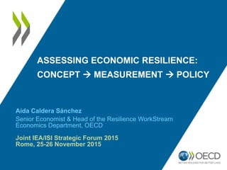
DEFINE
What’s a resilient economy?
How to minimise the costs of crises?
• Definition is general, supported by literature, and
operational for policy use
• Related OECD work:
• e.g. Ahrend and Goujard, 2012; Furceri et al. 2011
• e.g. de Serres and Drew, 2004; Duval et al. 2007
• 2014 OECD Ministerial Council Meeting
Can stop vulnerabilities
from building up
Can resist
adverse shocks
5. 5
FRAME
Which factors?
… increase vulnerability
to crises?
DIMENSION 1
… reduce the amplitude of
downturns?
… speed up recovery?
DIMENSION 2
• Price & wage flexibility
• Diversified production & export base
• High entry & exit
• Resource reallocation
• …
• Financial sector imbalances
• Asset market misalignments
• External sector imbalances
• Fiscal imbalances
• …
Economic structure, policies and institutions
6. • Reviewed early warning literature
– Röhn et al. (2015) discusses vulnerabilities preceding crises
• Shocks are difficult to predict and can arise from a
variety of sources
– Implication: Need to monitor vulnerabilities
• A new dataset of indicators
– Identify areas where vulnerabilities are building up
• Vulnerability indicators dashboard
– 34 OECD, BRIICS (Brazil, Russian Federation, India, Indonesia,
China, and South Africa), Colombia, Costa Rica, Latvia and
Lithuania.
– 1970 and 2014 or latest
– Publicly available sources (OECD, IMF, BIS)
– 6 areas 6
MEASURE
7. Vulnerabilities
Domestic side
Trade
channel
Financial sector
Leverage and risk taking
Liquidity and currency mismatches
Interconnectedness and common exposures
External sector
Unsustainable current account balances
Exchange rate misalignments
Public sector
Solvency risk
Long-term trends (e.g. ageing)
Fiscal uncertainty (e.g. contingent liabilities)
International
spillovers,
contagion and
global risks
Confidence channel
International side
Asset markets
Housing booms
Stock market booms
Non-financial sector
Excessive household debt
Excessive corporate debt
Data publicly available:
OECD Economic
Resilience Website
A bird’s eye view on 6 areas covered by dashboard of vulnerability indicators
Financial channel
8. Strong private credit growth
is a robust indicator of banking crises
8
-15
-10
-5
0
5
10
15
20
25
30
-40 -36 -32 -28 -24 -20 -16 -12 -8 -4 0 4 8 12 16 20 24 28 32 36 40
Private credit / GDP
Quarters since the start of the crisis
Point estimate 95% confidence interval
Note: The solid line shows the average percentage point change in private credit in per cent of GDP 10 years
before and 10 years after a banking crisis relative to normal times. The point estimate (solid line) and
confidence interval (dashed lines) are obtained by a difference in difference panel estimation controlling for
country and time fixed effects. Source: Röhn et al. (2015).
9. Real estate market downturns
are often associated with banking crises
9
-10
-5
0
5
10
15
20
-40 -36 -32 -28 -24 -20 -16 -12 -8 -4 0 4 8 12 16 20 24 28 32 36 40
Real houseprice index
Quarters sincethe start of the crisis
Point estimate 95% confidence interval
Note: The solid line shows the average percentage point change in real house prices 10 years before and 10 years after a
banking crisis relative to normal times. The point estimate (solid line) and confidence interval (dashed lines) are
obtained by a difference in difference panel estimation controlling for country and time fixed effects. Source: Röhn et al.
(2015).
10. Growing current account deficits
robust indicators of crises
10
-10
-5
0
5
10
15
20
-40 -36 -32 -28 -24 -20 -16 -12 -8 -4 0 4 8 12 16 20 24 28 32 36 40
Real houseprice index
Quarters sincethe start of the crisis
Point estimate 95% confidence interval
Note: The solid line shows the average percentage point change in the current account deficit in per cent of GDP 10 years
before and 10 years after a crisis (banking, sovereign debt or currency) relative to normal times. The point estimate
(solid line) and confidence interval (dashed lines) are obtained by a difference in difference panel estimation controlling
for country and time fixed effects. Source: Röhn et al. (2015).
11. EMPIRICAL ANALYSIS #1
Are the vulnerability indicators useful in
predicting severe recessions and crises?
11
12. • Testing if vulnerability indicators signal severe recessions and crises
– Severe recessions and banking, currency or sovereign debt crises in
OECD economies between 1970 and 2014 (Hermansen and Röhn,
2015)
– Based on well-known “signaling approach” (Kaminsky et al. 1998)
• Results
– Majority of indicators useful (in-sample and out- of-sample)
– Global risk indicators more useful than domestic indicators
– In domestic areas
• Indicators of asset market imbalances perform well (real house
and equity prices, house price-to-income, and house price-to-rent)
• Credit variables useful in signaling upcoming banking crises and
in predicting the Global Crisis (out-of-sample)
• Indicators of external imbalances (e.g. current-account
balances, official reserves) perform well in some specifications
Are vulnerability indicators useful?
12
13. • Vulnerability indicators valuable for monitoring country risks
• Need to be complemented with other tools
– In-depths assessments, expert judgment, etc.
• Vulnerabilities can interact and reinforce each other
• Difficulties to assess some vulnerabilities in real time
• Data gaps
– Financial market: interconnectedness of financial institutions, shadow
banking
– Non-financial sector: underwriting standards, micro-level data on
leverage households, firms’ balance sheets
– Asset markets: house price data, commercial real estate
– Public sector: government contingent liabilities
– Better measures of global risks, international spillovers and contagion
Conclusions
13
15. • Literature assessing drivers of deep downturns
• Acemoglu et al., 2014; Stiglitz, 2015
• We use quantile regression techniques to characterise the
likelihood of extraordinary negative GDP outcomes as a function of
observable macroeconomic and policy factors
• GDP-at-Risk: measure of macroeconomic risk.
GDP at risk: The approach
15
0
GDP-at-Risk
(max GDP loss with 95% prob.)
GDP
Tail
events
GDP at Risk
lower qth (e.g. the 5th)
quantile of the GDP
distribution
16. Standard approaches to measuring volatility
do not fully characterise the tails
16
=> GDP distributions have fat tails
Quantile-Quantile plots
17. • No need to rely on (ex-post) crises definition or to date booms
and recessions.
• Can focus on extreme output events.
• Can assess (within the same framework) if the drivers of
extreme negative output events similar to drivers of extreme
positive output events.
• Benefits compared to approaches assessing macro risks with
volatility:
– Volatility captures not only large, abrupt contractions, but also
frequent milder shocks
– Standard deviation (SD) is symmetric.
– Evidence of thick tails in the GDP distribution =>SD not such a
good measure of tail risks =>risk varies across economies with
similar SD.
Advantages
17
18. • Quantile regression techniques to link GDP-at-risk
with factors (Xt) that influence the GDP distribution.
𝑄 𝜏 𝑦𝑡+1|𝑋𝑡 = 𝑋𝑡 𝛽(𝜏)
𝛃 𝛕 : marginal change in the τth
quantile of y due to a marginal
change in X (e.g. for 𝜏 = 0.05 it gives the impact on the 5-percent
GDP-at-risk).
𝒚: GDP deviation from trend 4-, 8- and 12-quarters ahead.
𝑿: factors that can influence the GDP distribution (e.g. risk
factors or policies)
18
Methodology
Varies across
quantiles
19. 19
A different impact of risk factors across
quantiles of the GDP distribution
Beta(t)-coefficientonX
The betas vary across
quantiles
Estimates of the impact of private credit deviation
from trend on GDP deviation from trend
Note: the dotted lines (shaded areas) indicate the 95% confidence interval around the OLS (quantile)
coefficient. Data: 42 OECD and non-OECD countries, 1960Q1 where possible to 2014Q4.
OLS coefficient Quantile regression coefficient
20. Credit booms can increase
downside risks
20
Fitted quantile regression lines for the 5th, 50th and 95th
percentiles
As a credit boom intensifies,
higher probability of extreme
outcomes: higher GDP at risk
Note: This figure illustrates the conditional impact of a credit boom on the distribution of future quarterly GDP
deviations from trend. Dataset includes 42 OECD and non-OECD countries, 1960Q1 where possible to 2014Q4 .
21. Preliminary results
• Some risk factors (credit booms, housing booms, current
account imbalances) increase GDP-at-risk.
Next steps
• Refinements and robustness checks
– Control for GDP covariates; etc
• Role of structural policies: Which policy settings are
related to bad booms? How policy settings are related to
severity of bad outcome? Which policies to deal with a
bust?
Way forward…
21
22. Fill data gaps: Housing market policies, taxation, lending
standards, bankruptcy regulation ..
Which policy settings linked to bad booms? How policy settings
are related to severity of bad outcome? Which policies to deal
with a bust? ….
Policy lessons into OECD Economic Surveys, Economic
Outlook, Going for Growth…
Economic Resilience WorkStream:
What’s next?
22
MEASURE
ANALYSE
INTEGRATE
25. Housing booms can increase
downside risks
25
As a housing-boom intensifies, higher
probability of extreme outcomes:
higher GDP at risk
Fitted quantile regression lines for the 5th, 50th and 95th
percentiles
Note: This figure illustrates the conditional impact of a housing boom on the distribution of future quarterly GDP
deviations from trend. Dataset includes 42 OECD and non-OECD countries, 1960Q1 where possible to 2014Q4 .
26. Current account imbalances can
increase downside risks
26
Fitted quantile regression lines for the 5th, 50th and 95th
percentiles
As CA imbalances intensify, higher
probability of extreme outcomes: higher
GDP at risk
Note: This figure illustrates the conditional impact of an increasing CA imbalance on the distribution of future quarterly GDP
deviations from trend. Dataset includes 42 OECD and non-OECD countries, 1960Q1 where possible to 2014Q4 .
Editor's Notes
Develop a conceptual framework for assessing countries’ resilience to macroeconomic shocks.
Identify analytically robust indicators to measure vulnerabilities.
Analyse how differences in resilience are related to differences in policies and structural settings.
Deliver policy advise on strengthening countries’ resilience to macroeconomic shocks.
Resilience: typically understood as the capacity to absorb a shock and bounce back
Definition needs to be general, build on the body of available literature, allow for its operational use for policy.
Two aspects highlighted in previous OECD work:
Resilient economy, one with the capacity to contain vulnerabilities that can lead to costly crises (e.g. currency, banking, debt crisis) (e.g. Ahrend and Goujard, 2012; Furceri et al. 2011).
Resilient economy, one that withstands an adverse shock better and returns back faster to the pre-shock trend growth (e.g. de Serres and Drew, 2004; Duval et al. 2007).
Hermansen and Röhn (2015) test how useful indicators would have been in signaling in advance severe recessions and crises (banking, currency or sovereign debt crises) in OECD economies between 1970 and 2014.
Used a well-known methodology, “signaling approach” (Kaminsky et al. 1998).
Findings:
Majority of indicators useful in signaling severed recessions and crises (in-sample and out- of-sample).
Global risk indicators relatively more useful than domestic indicators in signaling severe recessions.
In the domestic areas, indicators of asset market imbalances (real house and equity prices, house price-to-income, and house price-to-rent), perform well.
Domestic credit variables useful in signaling upcoming banking crises and in predicting the Global Crisis out-of-sample.
Indicators of external imbalances (e.g. current-account balances, official reserves) perform well in certain specifications.