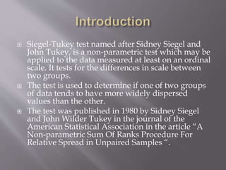
Siegel-Tukey test named after Sidney Siegel and John Tukey, is a non-parametric test which may be applied to the data measured at least on an ordinal scale. It tests for the differences in scale between two groups. The test is used to determine if one of two groups of data tends to have more widely dispersed values than the other. The test was published in 1980 by Sidney Siegel and John Wilder Tukey in the journal of the American Statistical Association in the article “A Non-parametric Sum Of Ranks Procedure For Relative Spread in Unpaired Samples “.

1.  Siegel-Tukey test named after Sidney Siegel and
John Tukey, is a non-parametric test which may be
applied to the data measured at least on an ordinal
scale. It tests for the differences in scale between
two groups.
 The test is used to determine if one of two groups
of data tends to have more widely dispersed
values than the other.
 The test was published in 1980 by Sidney Siegel
and John Wilder Tukey in the journal of the
American Statistical Association in the article “A
Non-parametric Sum Of Ranks Procedure For
Relative Spread in Unpaired Samples “.

2.  Each sample has been randomly selected from
the population.
 The two samples are independent of one
another.
 The level of measurement the data represent is
at least ordinal.
 The two populations from which the samples
are derived have equal medians.

3.  Null hypothesis
 H0 : δ2
A = δ
2
B
 When the sample sizes are equal , then sum of the
ranks also will be equal.
 ԐR1 = ԐR2
 Alternate hypothesis
 H1: δ2
A ≠ δ
2
B

4. 2) α=0.05
3) Test statistic
Siegel-Tukey test
4) Calculations
By combining the groups. The ranking is done by
alternate extremes (rank 1 is lowest, 2 and 3 are the
two highest, 4 and 5 are the two next lowest etc)
Sum the rank of first and second group, after this
procedure apply Mann-Whitney U test to find out
the U value.

5.  U1 = n1n2+n1(n1+1)/2‒ ԐR1
 U2 = n1n2+n2(n2+1)‒ԐR2
 U = Min( U1,U2)
5)Critical region
Ucal ˂ Utab ˂ Ucal
6) Conclusion
Accept or reject H0

6. Two plastics each produced by a different process
were tested for ultimate strength. The
measurement shown below represent breaking
load in units of 1000 pounds per square inch.
Plastic 1: 15.3, 18.7, 22.3, 17.6, 15.1, 14.8
Plastic 2: 21.2, 22.4, 18.3, 19.3, 17.1, 27.7
Use Siegel-Tukey test to test the hypothesis that
: δ2
1 = δ
2
2

7. 1) H0 : : δ2
1 = δ
2
2
H1: δ2
1 ≠ δ
2
2
2) α=0.05
3) Test statistic
Siegel-Tukey test
4) Calculations
Arrange combine samples in ascending
order,

8.  14.8, 15.1, 15.3, 17.1, 17.6, 18.3, 18.7, 19.3,
 1 4 5 8 9 12 11 10
 21.2, 22.3, 22.4, 27.7
 7 6 3 2
 R1 = 1+4+5+9+11+6 = 36
 R2 = 8+12+10+7+3+2 = 42
 U1 = n1n2+n1(n1+1)/2‒ ԐR1
 = 36+6( 6+1 ) /2 – 36
 =21

9.  U2 = n1n2- U1
 = 36 – 21
 U2 = 15
 U = min ( U1 , U2 )
 U = min ( 21 , 15 )
 U = 15
5) Critical region
If U cal lies between 5 and 31 we accept H0,
otherwise we will reject

10. 6) Conclusion
As the calculated value of U lies in the interval 5
and 31. So, we accept the null hypothesis.

11. X1 : 10, 10, 9, 1, 0, 0
X2 : 6, 6, 5, 5, 4, 4
SOLUTION:
1) H0 : : δ2
1 = δ
2
2
H1: δ2
1 ≠ δ
2
2
2) α=0.05
3) Test statistic
Siegel-Tukey test

12. 4) Calculations
Arrange combine samples in ascending order,
 Arrange data set 0, 0, 1, 4, 4, 5, 5, 6, 6, 9, 10, 10
 Ranks 1 4 5 8 9 12 11 10 7 6 3 2
 Tied adjusted rank 2.5, 2.5, 5, 8.5, 8.5, 11.5, 11.5, 8.5,
8.5, 6, 2.5, 2.5
 R1 = 2.5+2.5+6+5+2.5+2.5 = 21

13.  R2 = 8.5 +8.5+11.5+11.5+8.5+8.5 = 57
 U1 = n1n2+n1(n1+1)/2‒ ԐR1
 U1 = 36+6( 6+1)/2 – 21
 U1 = 36+21 – 21
 U1 = 36
 U2 = n1n2 – U1
 U2 = 36 – 36
 U2 = 0

14.  U = min ( U1,U2 )
 U = min (36,0)
 U = 0
5) Critical region
If U cal lies between 5 and 31 we will accept,
otherwise we will reject
6) Conclusion
As the calculated value of U does not lie in the
interval 5 and 31. So, we will reject the null
hypothesis.

15. If the sample size is greater than 8 and there are tied
ranks in the data. We will use the formula
𝑧 =
𝑢−𝑛1𝑛2
2
𝑛1𝑛2 𝑛1+𝑛2+1
12
−
𝑛1𝑛2 Σs 𝑡3−𝑡
12𝑛1𝑛2 𝑛1+𝑛2−1
Where s denotes the no of pair of ties
and t denotes no of tied ranks

16.  Group 1: 3.1, 5.3, 6.4, 6.2, 3.8, 7.5, 5.8, 4.3, 5.9, 4.9
 Group 2: 9, 5.6, 6.3, 8.5, 4.6, 7.1, 5.5, 7.9, 6.8, 5.7,
8.9
Solution:
1) H0 : : δ2
1 = δ
2
2
H1: δ2
1 ≠ δ
2
2
2) α=0.05
3) Test statistic
Siegel-Tukey test

17. 4) Calculations
Arrange combine samples in ascending order
 3.1, 3.8, 4.3, 4.6, 4.9, 5.3, 5.5, 5.6, 5.7, 5.8,
 1 4 5 8 9 12 13 16 17 20
 5.9, 6.2, 6.3, 6.4, 6,8, 7.1, 7.5, 7.9, 8.5, 8.9, 9.0
 21 19 18 15 14 11 10 7 6 3 2
R1 = 1+4+5+9+12+20+21+19+15+10 = 116

18. R2 = 8+13+16+17+18+14+11+7+6+3+2 = 115
U1 = n1n2+n1(n1+1)/2‒ ԐR1
U1 = 10(11)+10(10+1)/2 – 116
U1 = 149
U2 = n1n2+n2(n2+1)‒ԐR2
U2 = 10(11)+11(11+1)/2 – 115
U2 = 61

19.  U=min( U1,U2 )
 U=min( 149,61 )
 U=61
 𝑧 =
𝑢−
𝑛1𝑛2
2
𝑛1𝑛2 𝑛1+𝑛2+1
12
 𝑧 =
61−
10(11)
2
10(11) 10+11+1
12

20.  Z = 0.42
5) Critical region
If Zcal ≥ Ztab we reject our null hypothesis
6) Conclusion
Since calculated value is less than tabulated value. So,
we accept the null hypothesis.

21. THANK
YOU