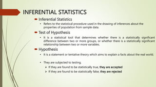
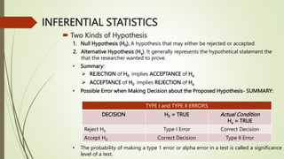
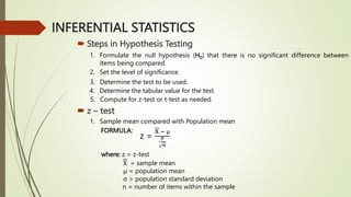
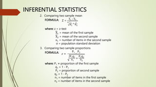
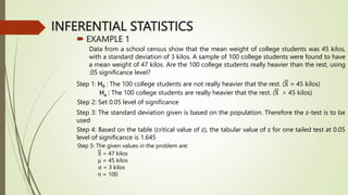
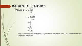
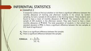
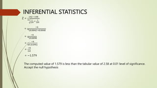
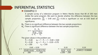
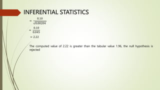
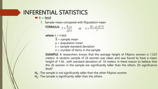
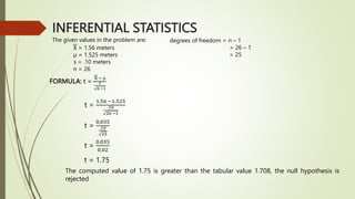
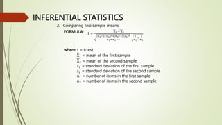
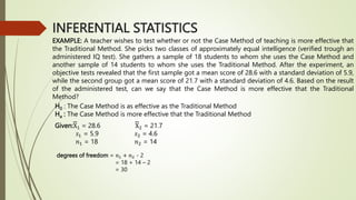
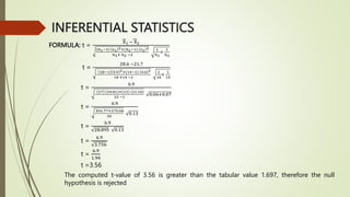
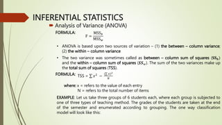
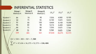
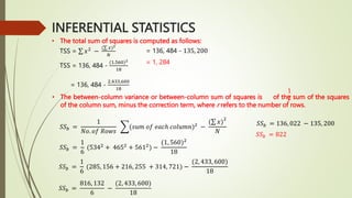
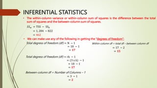
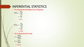
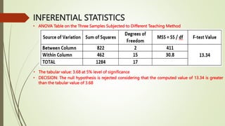
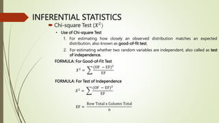
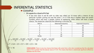
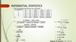
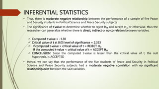
SlideShare a Scribd company logo
1 of 34
ADVANCE STATISTICS
Jemer M. Mabazza, LLB, PhD
Graduate School
Mallig Plains Colleges
INFERENTIAL STATISTICS
๏‚ด Inferential Statistics
โ€ข Refers to the statistical procedure used in the drawing of inferences about the
properties of population from sample data.
๏‚ด Test of Hypothesis
โ€ข It is a statistical tool that determines whether there is a statistically significant
difference between two or more groups, or whether there is a statistically significant
relationship between two or more variables.
๏‚ด Hypothesis
โ€ข It is a statement or tentative theory which aims to explain a facts about the real world.
โ€ข They are subjected to testing.
๏ƒ˜ If they are found to be statistically true, they are accepted
๏ƒ˜ If they are found to be statistically false, they are rejected
INFERENTIAL STATISTICS
๏‚ด Two Kinds of Hypothesis
1. Null Hypothesis (H0). A hypothesis that may either be rejected or accepted
2. Alternative Hypothesis (Ha). It generally represents the hypothetical statement the
that the researcher wanted to prove.
โ€ข Summary:
๏ƒ˜ REJECTION of H0 implies ACCEPTANCE of Ha
๏ƒ˜ ACCEPTANCE of H0 implies REJECTION of Ha
โ€ข Possible Error when Making Decision about the Proposed Hypothesis- SUMMARY:
TYPE I and TYPE II ERRORS
DECISION H0 = TRUE Actual Condition
Ha = TRUE
Reject H0 Type I Error Correct Decision
Accept H0 Correct Decision Type II Error
โ€ข The probability of making a type 1 error or alpha error in a test is called a significance
level of a test.
INFERENTIAL STATISTICS
๏‚ด Steps in Hypothesis Testing
1. Formulate the null hypothesis (H0) that there is no significant difference between
items being compared.
2. Set the level of significance.
3. Determine the test to be used.
4. Determine the tabular value for the test.
5. Compute for z-test or t-test as needed.
๏‚ด z โ€“ test
1. Sample mean compared with Population mean
FORMULA:
z =
X โˆ’ ยต
ฯƒ
๐‘›
where: z = z-test
X = sample mean
ยต = population mean
ฯƒ = population standard deviation
n = number of items within the sample
INFERENTIAL STATISTICS
2. Comparing two sample mean
FORMULA: Z =
X1 โˆ’ X2
ฯƒ 1
n1
+
1
n2
where: z = z-test
X1 = mean of the first sample
X2 = mean of the second sample
n1 = number of items in the second sample
ฯƒ = population standard deviation
3. Comparing two sample proportions
FORMULA:
where: P1 = proportion of the first sample
q1 = 1 - P1
P2 = proportion of second sample
q2 = 1 - P2
n1 = number of items in the first sample
n2 = number of items in the second sample
๐‘ง =
P1 โˆ’
P2
P1q1
n1
+
P2q2
n2
INFERENTIAL STATISTICS
๏‚ด EXAMPLE 1
Data from a school census show that the mean weight of college students was 45 kilos,
with a standard deviation of 3 kilos. A sample of 100 college students were found to have
a mean weight of 47 kilos. Are the 100 college students really heavier than the rest, using
.05 significance level?
Step 1: H0 : The 100 college students are not really heavier that the rest. (X = 45 kilos)
Ha : The 100 college students are really heavier that the rest. (X > 45 kilos)
Step 2: Set 0.05 level of significance
Step 3: The standard deviation given is based on the population. Therefore the z-test is to be
used
Step 4: Based on the table (critical value of z), the tabular value of z for one tailed test at 0.05
level of significance is 1.645
Step 5: The given values in the problem are:
X = 47 kilos
ยต = 45 kilos
ฯƒ = 3 kilos
n = 100
INFERENTIAL STATISTICS
FORMULA: z =
X โˆ’ ยต
ฯƒ
๐‘›
z =
47 โˆ’45
3
100
=
2
3
10
=
2
0.3
= 6.67
Step 6: The computed value of 6.67 is greater than the tabular value 1.645. Therefore, the null
hypothesis is rejected
INFERENTIAL STATISTICS
๏‚ด EXAMPLE 2
A researcher wishes to find out whether or not there is significant difference between the
monthly allowance of morning and afternoon students In his school. By random
sampling, he took a sample of 239 students in the morning session. These students were
found to have a mean of monthly allowance of โ‚ฑ142.00. The researcher also took a
sample of 209 students in the afternoon session. They were found to have a mean
monthly allowance of โ‚ฑ148.00. The total population of students in that school has a
standard deviation of โ‚ฑ40. Is there a significant difference between the two samples at
0.01 level of significance?
H0 : There is no significant difference between the samples
Ha : There is significant difference between the samples
FORMULA: Z =
X1 โˆ’ X2
ฯƒ 1
n1
+
1
n2
INFERENTIAL STATISTICS
Z =
142 โˆ’148
40 1
239
+
1
209
=
โˆ’6
40
0.0042 +0.0048
=
โˆ’6
40
0.0090
=
โˆ’6
40 (0.095)
=
โˆ’6
3.8
= โˆ’1.579
The computed value of 1.579 is less than the tabular value of 2.58 at 0.01 level of significance.
Accept the null hypothesis
INFERENTIAL STATISTICS
๏‚ด EXAMPLE 3
A sample survey of a television program in Metro Manila shows that 80 of 200 men
dislike the same program. We want to decide whether the difference between the two
sample proportion,
80
200
= 0.40 and
75
250
= 0.30, is significant or not at 0.05 level of
significance.
H0 : There is no significant difference between the two sample proportions
Ha : There is significant difference between the two sample proportions
The given values in the problem are:
P1 = 0.40 q1 = 1 - P1 = 1 โ€“ 0.40 = 0.60
P2 = 0.30 q2 = 1 - P2 = 1 โ€“ 0.30 = 0.70
n1 = 200 n2 = 250
๐‘ง =
P1 โˆ’
P2
P1q1
n1
+
P2q2
n2
๐‘ง =
0.40 โˆ’ 0.30
(0.40) (0.60)
200
+
(0.30) 0.70)
250
=
0.10
0.24
200
+
0.21
250
=
0.10
0.0012 + 0.00084
INFERENTIAL STATISTICS
=
0.10
0.00204
=
0.10
0.045
= 2.22
The computed value of 2.22 is greater than the tabular value 1.96, the null hypothesis is
rejected
INFERENTIAL STATISTICS
๏‚ด t โ€“ test
1. Sample mean compared with Population mean
FORMULA: t =
X โˆ’ ยต
๐‘ 
๐‘› โˆ’1
or t =
X โˆ’ ยต ๐‘› โˆ’1
๐‘ 
where: t = t-test
X = sample mean
ยต = population mean
s = sample standard deviation
n = number of items in the sample
EXAMPLE: A researchers knows that the average height of Filipino women is 1.525
meters. A random sample of 26 women was taken and was found to have a mean
height of 1.56 , with standard deviation of .10 meters. Is there reason to believe that
the 26 women in the sample are significantly taller than the others .05 significance
level?
H0 : The sample is not significantly taller than the other Filipino women
Ha : The sample is significantly taller than the others
INFERENTIAL STATISTICS
The given values in the problem are:
X = 1.56 meters
ยต = 1.525 meters
s = .10 meters
n = 26
degrees of freedom = n โ€“ 1
= 26 โ€“ 1
= 25
FORMULA: t =
X โˆ’ ยต
๐‘ 
๐‘› โˆ’1
t =
1.56 โˆ’1.525
.10
26 โˆ’1
t =
0.035
.10
25
t =
0.035
0.02
t = 1.75
The computed value of 1.75 is greater than the tabular value 1.708, the null hypothesis is
rejected
INFERENTIAL STATISTICS
2. Comparing two sample means
FORMULA: t =
X1 โˆ’ X2
(๐‘›1โˆ’1) ๐‘ 1
2+(๐‘›2โˆ’1) ๐‘ 2
2
๐‘›1+ ๐‘›2 โˆ’2
1
๐‘›1
+
1
๐‘›2
where: t = t-test
X1 = mean of the first sample
X2 = mean of the second sample
๐‘ 1 = standard deviation of the first sample
๐‘ 2 = standard deviation of the second sample
๐‘›1 = number of items in the first sample
๐‘›2 = number of items in the second sample
INFERENTIAL STATISTICS
EXAMPLE: A teacher wishes to test whether or not the Case Method of teaching is more effective that
the Traditional Method. She picks two classes of approximately equal intelligence (verified trough an
administered IQ test). She gathers a sample of 18 students to whom she uses the Case Method and
another sample of 14 students to whom she uses the Traditional Method. After the experiment, an
objective tests revealed that the first sample got a mean score of 28.6 with a standard deviation of 5.9,
while the second group got a mean score of 21.7 with a standard deviation of 4.6. Based on the result
of the administered test, can we say that the Case Method is more effective that the Traditional
Method?
H0 : The Case Method is as effective as the Traditional Method
Ha : The Case Method is more effective that the Traditional Method
Given:X1 = 28.6 X2 = 21.7
๐‘ 1 = 5.9 ๐‘ 2 = 4.6
๐‘›1 = 18 ๐‘›2 = 14
degrees of freedom = ๐‘›1 + ๐‘›2 - 2
= 18 + 14 โ€“ 2
= 30
INFERENTIAL STATISTICS
FORMULA: t =
X1 โˆ’ X2
(๐‘›1โˆ’1) ๐‘ 1
2+(๐‘›2โˆ’1) ๐‘ 2
2
๐‘›1+ ๐‘›2 โˆ’2
1
๐‘›1
+
1
๐‘›2
t =
28.6 โˆ’21.7
18โˆ’1 5.9 2+(14โˆ’1) 4.6 2
18 +14 โˆ’2
1
18
+
1
14
t =
6.9
17 (34.81)+(13) (21.16)
32 โˆ’2
0.06+0.07
t =
6.9
591.77+275.08
30
0.13
t =
6.9
28.895 0.13
t =
6.9
3.756
t =
6.9
1.94
t =3.56
The computed t-value of 3.56 is greater than the tabular value 1.697, therefore the null
hypothesis is rejected
INFERENTIAL STATISTICS
๏‚ด Analysis of Variance (ANOVA)
FORMULA:
F =
MSS๐‘
MSS๐‘ค
โ€ข ANOVA is based upon two sources of variation โ€“ (1) the between โ€“ column variance;
(2) the within โ€“ column variance
โ€ข The two variance was sometimes called as between โ€“ column sum of squares (๐’๐’๐’ƒ)
and the within โ€“ column sum of squares (๐‘บ๐‘บ๐‘ค). The sum of the two variances make up
the total sum of squares (TSS).
FORMULA: TSS = ๐‘ฅ2 โˆ’
( ๐‘ฅ)2
๐‘
where: x = refers to the value of each entry
N = refers to the total number of items
EXAMPLE: Let us take three groups of 6 students each, where each group is subjected to
one of three types of teaching method. The grades of the students are taken at the end
of the semester and enumerated according to grouping. The one way classification
model will look like this:
INFERENTIAL STATISTICS
Group I
Method A
Group II
Method B
Group III
Method C
Student 1
Student 2
Student 3
Student 4
Student 5
Student 6
84
90
92
96
84
88
70
75
90
80
75
75
90
95
100
98
88
90
(๐‘‹๐‘Ž)2 (๐‘‹๐‘)2
(๐‘‹๐‘)2
7,056
8,100
8,464
9,216
7,056
7,744
4,900
5,625
8,100
6,400
5,625
5,625
8,100
9,025
10,000
9,604
7,744
7,744
534 465 561 47,636 36,275 52,573
๐‘‹ = 534 + 465 + 561 = 1, 560
๐‘‹2 = 47, 636 + 36, 275 + 52, 573 = ๐Ÿ๐Ÿ‘๐Ÿ”, ๐Ÿ’๐Ÿ–๐Ÿ’
INFERENTIAL STATISTICS
โ€ข The total sum of squares is computed as follows:
TSS = 136, 484 -
(1,560)2
18
= 136, 484 -
2,433,600
18
= 136, 484 - 135, 200
= 1, 284
โ€ข The between-column variance or between-column sum of squares is of the sum of the squares
of the column sum, minus the correction term, where r refers to the number of rows.
1
๐‘Ÿ
๐‘†๐‘†๐‘ =
1
๐‘๐‘œ. ๐‘œ๐‘“ ๐‘…๐‘œ๐‘ค๐‘ 
(๐‘ ๐‘ข๐‘š ๐‘œ๐‘“ ๐‘’๐‘Ž๐‘โ„Ž ๐‘๐‘œ๐‘™๐‘ข๐‘š๐‘›)2
โˆ’
( ๐‘ฅ)
2
๐‘
๐‘†๐‘†๐‘ =
1
6
(5342
+ 4652
+ 5612
) โˆ’
(1, 560)2
18
๐‘†๐‘†๐‘ =
1
6
(285, 156 + 216, 255 + 314, 721) โˆ’
(2, 433, 600)
18
๐‘†๐‘†๐‘ =
816, 132
6
โˆ’
(2, 433, 600)
18
๐‘†๐‘†๐‘ = 136, 022 โˆ’ 135, 200
๐‘†๐‘†๐‘ = 822
TSS = ๐‘ฅ2
โˆ’
( ๐‘ฅ)2
๐‘
INFERENTIAL STATISTICS
โ€ข The within-column variance or within-column sum of squares is the difference between the total
sum of squares and the between-column sum of squares.
๐‘†๐‘†๐‘ค = TSS โˆ’ SS๐‘
= 1, 284 โˆ’ 822
= 462
โ€ข We can make use any of the following in getting the โ€œdegrees of freedomโ€:
Total degress of freedom (df) = N โˆ’ 1
= 18 โˆ’ 1
= ๐Ÿ๐Ÿ•
Total degress of freedom (df) = rk โˆ’ 1
= (3 x 6) โˆ’ 1
= 18 โˆ’ 1
= ๐Ÿ๐Ÿ•
Between-column df = Number of Columns โ€“ 1
= 3 โˆ’ 1
= ๐Ÿ
Within-column df = total df โ€“ between column df
= 17 โˆ’ 2
= ๐Ÿ๐Ÿ“
INFERENTIAL STATISTICS
โ€ข To compute for the Mean Sum of Squares
๐‘€๐‘†๐‘†๐‘ =
SS๐‘
df๐‘
=
822
2
= 411
๐‘€๐‘†๐‘†๐‘ค =
SS๐‘ค
df๐‘ค
=
462
15
= 30.8
โ€ข To compute for the F-test
F =
MSS๐‘
MSS๐‘ค
F =
411
30.8
= 13.34
INFERENTIAL STATISTICS
โ€ข ANOVA Table on the Three Samples Subjected to Different Teaching Method
โ€ข The tabular value: 3.68 at 5% level of significance
โ€ข DECISION: The null hypothesis is rejected considering that the computed value of 13.34 is greater
than the tabular value of 3.68
INFERENTIAL STATISTICS
๏‚ด Chi-square Test (๐‘ฟ๐Ÿ
)
โ€ข Use of Chi-square Test
1. For estimating how closely an observed distribution matches an expected
distribution, also known as good-of-fit test.
2. For estimating whether two random variables are independent, also called as test
of independence.
FORMULA: For Good-of-Fit Test
๐‘‹2
=
(OF โˆ’ EF)2
EF
FORMULA: For Test of Independence
๐‘‹2
=
(OF โˆ’ EF)2
EF
EF =
Row Total x Column Total
n
INFERENTIAL STATISTICS
๏‚ด EXAMPLE
โ€ข Chi-square for a Good-of-Fit Test
๏ƒผ A two dice (dice A and B) with six sides was rolled out 10 times with a chance of any
particular number coming out was the same: 1 in 6. If the dice is loaded, there are certain
numbers which will have a greater chance of appearing, while others will have a lower
chance. The researcher observed the following in one dice (A).
๐‘ฅ2
=
(18โˆ’10)2
10
+
(5โˆ’10)2
10
+
(9โˆ’10)2
10
+
(7โˆ’10)2
10
+
(5โˆ’10)2
10
+
(16โˆ’10)2
10
๐‘ฅ2 = 6.4 + 2.5 + 0.1 + 0.9 + 2.5 + 3.6
๐‘ฅ2 = 16 CONCLUSION: There is very low chance that these rolls came from a fair dice considering that the calculated
value of 16 is greater that the tabular value of 11.07. This means that there is statistically significant difference
between the two dices.
INFERENTIAL STATISTICS
โ€ข Chi-square Test for Independence
โ€ข Test the hypothesis that academic performance does not depend on IQ at 1% significance level.
โ€ข Degrees of Freedom (df) = (r โ€“ 1) (k โ€“ 1)
= (2 โ€“ 1) (3 โ€“ 1)
= 2
โ€ข COMPUTATION: Getting the ๐…๐’†
๏ƒผ Where ๐‘“๐‘œ = 31, ๐‘“๐‘’ =
32 x 80
100
= 25.6
๏ƒผ Where ๐‘“๐‘œ = 1, ๐‘“๐‘’ =
32 x 20
100
= 6.4
๏ƒผ Where ๐‘“๐‘œ = 45, ๐‘“๐‘’ =
49 x 80
100
= 39.20
๏ƒผ Where ๐‘“๐‘œ = 4, ๐‘“๐‘’ =
49 x 20
100
= 9.80
๏ƒผ Where ๐‘“๐‘œ = 4, ๐‘“๐‘’ =
19 x 80
100
= 15.2
๏ƒผ Where ๐‘“๐‘œ = 15, ๐‘“๐‘’ =
19 x 20
100
= 3.80
INFERENTIAL STATISTICS
โ€ข Replacing the above values into the chi-square formula, we shall have:
๐‘‹2 =
(OF โˆ’ EF)2
EF
๐‘‹2
=
(31 โˆ’25.6)2
25.6
+
(1 โˆ’6.4)2
6.4
+
(45 โˆ’39.2)2
39.2
+
(4 โˆ’9.80)2
9.80
+
(4 โˆ’15.2)2
15.2
+
(15 โˆ’3.80)2
3.80
๐‘‹2 =
29.16
25.6
+
29.16
6.4
+
33.64
39.2
+
33.64
9.80
+
125.44
15.2
+
125.44
3.80
๐‘‹2 = 1.139 + 4.556 + 0.858 + 3.433 + 8.253 + 33.011
๐‘‹2 = 51.25
โ€ข Since the computed Chi-square value of 51.25 is greater than the tabular value of 9.21, the null
hypothesis is rejected. For the 100 students, academic performance depends on IQ
INFERENTIAL STATISTICS
๏‚ด Simple Regression Analysis
โ€ข Regression analysis is concerned with the problem of estimation and forecasting.
๏ƒผ TYPES OF RELATIONSHIP
1. Direct Relationship. The slope of the line is positive because Y increases as X also
increases
2. Inverse Relationship. The slope of the line is negative because Y decreases as X also
increases
โ€ข Least Square Regression Line or LSRL is a statistical technique that analyses the
relationship between the independent and dependent variables.
๏ƒผ EQUATION:
Y = a + bX
๏ƒผ NORMAL EQUATIONS:
1. ฮฃY = aN + bฮฃX
2. ฮฃXY = aฮฃX + bฮฃ๐‘ฟ๐Ÿ
INFERENTIAL STATISTICS
WHERE: ฮฃY = sum of the values of Y, the dependent variable
N = the number of pairs of X and Y
ฮฃX = sum of the values of X, the independent variable
ฮฃXY = the sum of the column XY, which is derived by multiplying the paired values of X and Y
ฮฃ๐—๐Ÿ
= the sum of the column ๐—๐Ÿ
is derived by squaring the values of X
โ€ข Based on the given data of X and Y, we can determine all of the above which means
that the two normal equations now consist of a system of two linear equations with
two unknowns โ€“ a and b
โ€ข FORMULAS:
a=
๐šบ๐˜ ๐šบ๐—๐Ÿ โˆ’ ๐šบ๐— (๐œฎ๐‘ฟ๐’€)
๐ ๐œฎ๐—๐Ÿ โˆ’(๐œฎ๐—)๐Ÿ
b=
๐ ๐œฎ๐—๐˜ โˆ’ ๐œฎ๐— (๐œฎ๐˜)
๐ ๐œฎ๐—๐Ÿ โˆ’ (๐œฎ๐—)๐Ÿ
INFERENTIAL STATISTICS
โ€ข EXAMPLE:
X Y XY X2
1
3
4
6
8
9
11
14
56
1
2
4
4
5
7
8
8
40
1
6
16
24
40
63
88
126
1
9
16
36
64
81
121
196
364 524
a=
40 524 โˆ’ 56 (364)
8 524 โˆ’(56)2
a=
20960โˆ’20384
4192 โˆ’3136
a=
576
1056
= ๐ŸŽ. ๐Ÿ“๐Ÿ’
b=
8 364 โˆ’ 56 (40)
8 524 โˆ’ (56)2
b=
2912โˆ’2240
4192 โˆ’3136
b=
672
1056
= ๐ŸŽ. ๐Ÿ”๐Ÿ’
Y = 0.54 + 0.64 (16)
= 0.54 + 10.24
= 10.78
INFERENTIAL STATISTICS
๏‚ด Simple Correlation Analysis
โ€ข Correlation analysis concerned with the relationship in the changes of such variables.
โ€ข Degrees of correlation or relationship between two variables
1. Perfect correlation (negative and positive)
2. Some degrees of correlation (negative and positive)
3. No correlation
โ€ข The concept of correlation in terms of computed value is called correlation coefficient.
The value of the correlation coefficient ranges from -1 to +1.
โ€ข Pearson r test. The Pearson Product-Moment Coefficient of Correlation, otherwise
known as Pearson r is the most commonly used correlation coefficient.
โ€ข Pearson r, as the most widely used measure of correlation has two basic assumptions,
to wit:
1. The existence of linear relationship; and
2. The level of measurement of the data for the two variables are either in interval or
ratio scale.
INFERENTIAL STATISTICS
โ€ข The value of r (degree of linear relationship) can be interpreted according to the use of
range of values for the Pearson Product Moment of Correlation Coefficient, as follows:
โ€ข Notably, Pearson r is not a measure of causality. The significant of the obtained
correlation coefficient can be determined through the use of t-test for testing the
significance of r.
๐ญ = ๐ซ
๐ง โˆ’ ๐Ÿ
๐Ÿ โˆ’ ๐ซ๐Ÿ
WHERE: t = t-test
r = obtained Pearson r value
n = paired sample size
FORMULA:
Degree of freedom = n โ€“ 2
INFERENTIAL STATISTICS
FORMULA for Pearson r:
๐’“ =
๐ ๐šบ๐—๐˜ โˆ’ ๐šบ๐— (๐šบ๐˜)
๐ ๐œฎ๐—๐Ÿ โˆ’ (๐œฎ๐—)๐Ÿ ๐ ๐œฎ๐˜๐Ÿ โˆ’ (๐œฎ๐˜)๐Ÿ
Where: r = correlation coefficient
N = total number of pair variables
X = the first variable under study
Y = the second variable under study
EXAMPLE:
A researcher wants to find out about the relationship between the performance of a sample
of five Peace and Security students in Political Science and Peace Security subjects:
INFERENTIAL STATISTICS
โ€ข The computational solutions are as follows:
๐’“ =
๐Ÿ“ (๐Ÿ‘๐Ÿ—๐Ÿ—๐Ÿ’๐Ÿ’) โˆ’ ๐Ÿ’๐Ÿ๐Ÿ“ (๐Ÿ’๐Ÿ•๐ŸŽ)
๐Ÿ“ ๐Ÿ‘๐Ÿ”๐Ÿ๐Ÿ‘๐Ÿ“ โˆ’ (๐Ÿ’๐Ÿ๐Ÿ“)๐Ÿ ๐Ÿ“ ๐Ÿ’๐Ÿ’๐Ÿ๐Ÿ—๐ŸŽ โˆ’ (๐Ÿ’๐Ÿ•๐ŸŽ)๐Ÿ
=
๐Ÿ๐Ÿ—๐Ÿ—๐Ÿ•๐Ÿ๐ŸŽ โˆ’ ๐Ÿ๐Ÿ—๐Ÿ—๐Ÿ•๐Ÿ“๐ŸŽ
๐Ÿ๐Ÿ–๐ŸŽ๐Ÿ”๐Ÿ•๐Ÿ“ โˆ’ ๐Ÿ๐Ÿ–๐ŸŽ๐Ÿ”๐Ÿ๐Ÿ“ ๐Ÿ๐Ÿ๐ŸŽ๐Ÿ—๐Ÿ“๐ŸŽ โˆ’ ๐Ÿ๐Ÿ๐ŸŽ๐Ÿ—๐ŸŽ๐ŸŽ
=
โˆ’๐Ÿ‘๐ŸŽ
๐Ÿ“๐ŸŽ ๐Ÿ“๐ŸŽ
=
โˆ’๐Ÿ‘๐ŸŽ
๐Ÿ๐Ÿ“๐ŸŽ๐ŸŽ
=
โˆ’๐Ÿ‘๐ŸŽ
๐Ÿ“๐ŸŽ
= โˆ’๐ŸŽ. ๐Ÿ”๐ŸŽ
๐ญ = โˆ’๐ŸŽ. ๐Ÿ”๐ŸŽ
๐Ÿ“ โˆ’ ๐Ÿ
๐Ÿ โˆ’ (โˆ’๐ŸŽ. ๐Ÿ”๐ŸŽ)๐Ÿ
= โˆ’๐ŸŽ. ๐Ÿ”๐ŸŽ
๐Ÿ‘
๐Ÿ โˆ’ ๐ŸŽ. ๐Ÿ‘๐Ÿ”
= โˆ’๐ŸŽ. ๐Ÿ”๐ŸŽ
๐Ÿ‘
๐ŸŽ. ๐Ÿ”๐Ÿ’
= โˆ’๐ŸŽ. ๐Ÿ”๐ŸŽ ๐Ÿ’. ๐Ÿ”๐Ÿ–๐Ÿ•๐Ÿ“
= โˆ’๐ŸŽ. ๐Ÿ”๐ŸŽ (2.165)
= โˆ’๐Ÿ. ๐Ÿ๐Ÿ—๐Ÿ—
Degree of freedom = 5 โ€“ 2 = 3
INFERENTIAL STATISTICS
โ€ข Thus, there is moderate negative relationship between the performance of a sample of five Peace
and Security students in Political Science and Peace Security subjects
โ€ข The significance of t-value to determine whether to reject ๐‡๐Ž and accept ๐‡๐š or otherwise, thus the
researcher can generalize whether there is direct, indirect or no correlation between variables.
๏ƒผ Computed t value = -1.30
๏ƒผ Critical value of t at 0.05 level of significance = 2.353
๏ƒผ If computed t-value > critical value of t = REJECT ๐‡๐Ž
If the computed t-value < critical value of t = ACCEPT ๐‡๐Ž
๏ƒผ CONCLUSION: Since the computed t-value is lesser than the critical value of t, the null
hypothesis, is ACCEPTED
โ€ข Hence, we can say that the performance of the five students of Peace and Security in Political
Science and Peace Security subjects had a moderate negative correlation with no significant
relationship exist between the said variables.

More Related Content

What's hot

PEARSON'CORRELATION
PEARSON'CORRELATION PEARSON'CORRELATION
PEARSON'CORRELATION Kasi Valaparla
ย 
Difference between grouped and ungrouped data
Difference between grouped and ungrouped dataDifference between grouped and ungrouped data
Difference between grouped and ungrouped dataAtiq Rehman
ย 
frequency distribution table
frequency distribution tablefrequency distribution table
frequency distribution tableMonie Ali
ย 
CABT SHS Statistics & Probability - Estimation of Parameters (intro)
CABT SHS Statistics & Probability -  Estimation of Parameters (intro)CABT SHS Statistics & Probability -  Estimation of Parameters (intro)
CABT SHS Statistics & Probability - Estimation of Parameters (intro)Gilbert Joseph Abueg
ย 
Slovin's formula
Slovin's formulaSlovin's formula
Slovin's formulaschool
ย 
G7 Math Q4-Week 1- Uses of Statistics.ppt
G7 Math Q4-Week 1- Uses of Statistics.pptG7 Math Q4-Week 1- Uses of Statistics.ppt
G7 Math Q4-Week 1- Uses of Statistics.pptArnoldMillones4
ย 
Mean, Median, Mode: Measures of Central Tendency
Mean, Median, Mode: Measures of Central Tendency Mean, Median, Mode: Measures of Central Tendency
Mean, Median, Mode: Measures of Central Tendency Jan Nah
ย 
Measures of central tendency (ungrouped data)
Measures of central tendency (ungrouped data)Measures of central tendency (ungrouped data)
Measures of central tendency (ungrouped data)LilianneSoriano
ย 
Measures of variability
Measures of variabilityMeasures of variability
Measures of variabilityjennytuazon01630
ย 
QUARTILES, DECILES AND PERCENTILES
QUARTILES, DECILES  AND PERCENTILESQUARTILES, DECILES  AND PERCENTILES
QUARTILES, DECILES AND PERCENTILESMARIA KATRINA MACAPAZ
ย 
parametric test of difference z test f test one-way_two-way_anova
parametric test of difference z test f test one-way_two-way_anova parametric test of difference z test f test one-way_two-way_anova
parametric test of difference z test f test one-way_two-way_anova Tess Anoza
ย 
1.1 mean, variance and standard deviation
1.1 mean, variance and standard deviation1.1 mean, variance and standard deviation
1.1 mean, variance and standard deviationONE Virtual Services
ย 
Data gathering
Data gatheringData gathering
Data gatheringChie Pegollo
ย 
Correlational research
Correlational researchCorrelational research
Correlational researchJijo G John
ย 
statistical estimation
statistical estimationstatistical estimation
statistical estimationAmish Akbar
ย 
Probability and statistics
Probability and statisticsProbability and statistics
Probability and statisticsFatima Bianca Gueco
ย 
The nature of probability and statistics
The nature of probability and statisticsThe nature of probability and statistics
The nature of probability and statisticsSan Benito CISD
ย 
Module 1 statistics
Module 1   statisticsModule 1   statistics
Module 1 statisticsdionesioable
ย 

What's hot (20)

PEARSON'CORRELATION
PEARSON'CORRELATION PEARSON'CORRELATION
PEARSON'CORRELATION
ย 
Difference between grouped and ungrouped data
Difference between grouped and ungrouped dataDifference between grouped and ungrouped data
Difference between grouped and ungrouped data
ย 
frequency distribution table
frequency distribution tablefrequency distribution table
frequency distribution table
ย 
CABT SHS Statistics & Probability - Estimation of Parameters (intro)
CABT SHS Statistics & Probability -  Estimation of Parameters (intro)CABT SHS Statistics & Probability -  Estimation of Parameters (intro)
CABT SHS Statistics & Probability - Estimation of Parameters (intro)
ย 
Slovin's formula
Slovin's formulaSlovin's formula
Slovin's formula
ย 
Mean for Grouped Data
Mean for Grouped DataMean for Grouped Data
Mean for Grouped Data
ย 
G7 Math Q4-Week 1- Uses of Statistics.ppt
G7 Math Q4-Week 1- Uses of Statistics.pptG7 Math Q4-Week 1- Uses of Statistics.ppt
G7 Math Q4-Week 1- Uses of Statistics.ppt
ย 
Mean, Median, Mode: Measures of Central Tendency
Mean, Median, Mode: Measures of Central Tendency Mean, Median, Mode: Measures of Central Tendency
Mean, Median, Mode: Measures of Central Tendency
ย 
Measures of central tendency (ungrouped data)
Measures of central tendency (ungrouped data)Measures of central tendency (ungrouped data)
Measures of central tendency (ungrouped data)
ย 
Measures of variability
Measures of variabilityMeasures of variability
Measures of variability
ย 
QUARTILES, DECILES AND PERCENTILES
QUARTILES, DECILES  AND PERCENTILESQUARTILES, DECILES  AND PERCENTILES
QUARTILES, DECILES AND PERCENTILES
ย 
Chapter 9-METHODS OF DATA COLLECTION
Chapter 9-METHODS OF DATA COLLECTIONChapter 9-METHODS OF DATA COLLECTION
Chapter 9-METHODS OF DATA COLLECTION
ย 
parametric test of difference z test f test one-way_two-way_anova
parametric test of difference z test f test one-way_two-way_anova parametric test of difference z test f test one-way_two-way_anova
parametric test of difference z test f test one-way_two-way_anova
ย 
1.1 mean, variance and standard deviation
1.1 mean, variance and standard deviation1.1 mean, variance and standard deviation
1.1 mean, variance and standard deviation
ย 
Data gathering
Data gatheringData gathering
Data gathering
ย 
Correlational research
Correlational researchCorrelational research
Correlational research
ย 
statistical estimation
statistical estimationstatistical estimation
statistical estimation
ย 
Probability and statistics
Probability and statisticsProbability and statistics
Probability and statistics
ย 
The nature of probability and statistics
The nature of probability and statisticsThe nature of probability and statistics
The nature of probability and statistics
ย 
Module 1 statistics
Module 1   statisticsModule 1   statistics
Module 1 statistics
ย 

Similar to Advance Statistics Techniques for Data Analysis

Statistical analysis.pptx
Statistical analysis.pptxStatistical analysis.pptx
Statistical analysis.pptxChinna Chadayan
ย 
Analysis of variance (ANOVA)
Analysis of variance (ANOVA)Analysis of variance (ANOVA)
Analysis of variance (ANOVA)Sneh Kumari
ย 
inferentialstatistics-210411214248.pdf
inferentialstatistics-210411214248.pdfinferentialstatistics-210411214248.pdf
inferentialstatistics-210411214248.pdfChenPalaruan
ย 
Inferential statistics
Inferential statisticsInferential statistics
Inferential statisticsDalia El-Shafei
ย 
Lecture 11 Paired t test.pptx
Lecture 11 Paired t test.pptxLecture 11 Paired t test.pptx
Lecture 11 Paired t test.pptxshakirRahman10
ย 
Chapter 7Hypothesis Testing ProceduresLearning.docx
Chapter 7Hypothesis Testing ProceduresLearning.docxChapter 7Hypothesis Testing ProceduresLearning.docx
Chapter 7Hypothesis Testing ProceduresLearning.docxmccormicknadine86
ย 
Non parametrics tests
Non parametrics testsNon parametrics tests
Non parametrics testsrodrick koome
ย 
Statistical analysis
Statistical  analysisStatistical  analysis
Statistical analysisPrincy Francis M
ย 
Test of significance
Test of significanceTest of significance
Test of significanceDr. Imran Zaheer
ย 
Sampling distribution.pptx
Sampling distribution.pptxSampling distribution.pptx
Sampling distribution.pptxssusera0e0e9
ย 
Central Tendency & Dispersion
Central Tendency & DispersionCentral Tendency & Dispersion
Central Tendency & DispersionBirinder Singh Gulati
ย 
Str t-test1
Str   t-test1Str   t-test1
Str t-test1iamkim
ย 
NON-PARAMETRIC TESTS.pptx
NON-PARAMETRIC TESTS.pptxNON-PARAMETRIC TESTS.pptx
NON-PARAMETRIC TESTS.pptxDrLasya
ย 
In a left-tailed test comparing two means with variances unknown b.docx
In a left-tailed test comparing two means with variances unknown b.docxIn a left-tailed test comparing two means with variances unknown b.docx
In a left-tailed test comparing two means with variances unknown b.docxbradburgess22840
ย 
Hypothesis_testing,regarding software engineering
Hypothesis_testing,regarding software engineeringHypothesis_testing,regarding software engineering
Hypothesis_testing,regarding software engineeringTallapelliSharanya01
ย 
UNIT 5.pdf
UNIT 5.pdfUNIT 5.pdf
UNIT 5.pdfRajaRokkala
ย 
Test of significance in Statistics
Test of significance in StatisticsTest of significance in Statistics
Test of significance in StatisticsVikash Keshri
ย 

Similar to Advance Statistics Techniques for Data Analysis (20)

Statistical analysis.pptx
Statistical analysis.pptxStatistical analysis.pptx
Statistical analysis.pptx
ย 
Analysis of variance (ANOVA)
Analysis of variance (ANOVA)Analysis of variance (ANOVA)
Analysis of variance (ANOVA)
ย 
inferentialstatistics-210411214248.pdf
inferentialstatistics-210411214248.pdfinferentialstatistics-210411214248.pdf
inferentialstatistics-210411214248.pdf
ย 
Inferential statistics
Inferential statisticsInferential statistics
Inferential statistics
ย 
Lecture 11 Paired t test.pptx
Lecture 11 Paired t test.pptxLecture 11 Paired t test.pptx
Lecture 11 Paired t test.pptx
ย 
Chapter 7Hypothesis Testing ProceduresLearning.docx
Chapter 7Hypothesis Testing ProceduresLearning.docxChapter 7Hypothesis Testing ProceduresLearning.docx
Chapter 7Hypothesis Testing ProceduresLearning.docx
ย 
Non parametrics tests
Non parametrics testsNon parametrics tests
Non parametrics tests
ย 
Statistical analysis
Statistical  analysisStatistical  analysis
Statistical analysis
ย 
Test of significance
Test of significanceTest of significance
Test of significance
ย 
Sampling distribution.pptx
Sampling distribution.pptxSampling distribution.pptx
Sampling distribution.pptx
ย 
Statistical analysis by iswar
Statistical analysis by iswarStatistical analysis by iswar
Statistical analysis by iswar
ย 
Central Tendency & Dispersion
Central Tendency & DispersionCentral Tendency & Dispersion
Central Tendency & Dispersion
ย 
Parametric tests
Parametric testsParametric tests
Parametric tests
ย 
Str t-test1
Str   t-test1Str   t-test1
Str t-test1
ย 
NON-PARAMETRIC TESTS.pptx
NON-PARAMETRIC TESTS.pptxNON-PARAMETRIC TESTS.pptx
NON-PARAMETRIC TESTS.pptx
ย 
In a left-tailed test comparing two means with variances unknown b.docx
In a left-tailed test comparing two means with variances unknown b.docxIn a left-tailed test comparing two means with variances unknown b.docx
In a left-tailed test comparing two means with variances unknown b.docx
ย 
Hypothesis_testing,regarding software engineering
Hypothesis_testing,regarding software engineeringHypothesis_testing,regarding software engineering
Hypothesis_testing,regarding software engineering
ย 
UNIT 5.pdf
UNIT 5.pdfUNIT 5.pdf
UNIT 5.pdf
ย 
Test of significance in Statistics
Test of significance in StatisticsTest of significance in Statistics
Test of significance in Statistics
ย 
Swayam
SwayamSwayam
Swayam
ย 

Recently uploaded

Saket, (-DELHI )+91-9654467111-(=)CHEAP Call Girls in Escorts Service Saket C...
Saket, (-DELHI )+91-9654467111-(=)CHEAP Call Girls in Escorts Service Saket C...Saket, (-DELHI )+91-9654467111-(=)CHEAP Call Girls in Escorts Service Saket C...
Saket, (-DELHI )+91-9654467111-(=)CHEAP Call Girls in Escorts Service Saket C...Sapana Sha
ย 
Call Girls In Noida City Center Metro 24/7โœก๏ธ9711147426โœก๏ธ Escorts Service
Call Girls In Noida City Center Metro 24/7โœก๏ธ9711147426โœก๏ธ Escorts ServiceCall Girls In Noida City Center Metro 24/7โœก๏ธ9711147426โœก๏ธ Escorts Service
Call Girls In Noida City Center Metro 24/7โœก๏ธ9711147426โœก๏ธ Escorts Servicejennyeacort
ย 
Call Girls In Mahipalpur O9654467111 Escorts Service
Call Girls In Mahipalpur O9654467111  Escorts ServiceCall Girls In Mahipalpur O9654467111  Escorts Service
Call Girls In Mahipalpur O9654467111 Escorts ServiceSapana Sha
ย 
Call Girls in Defence Colony Delhi ๐Ÿ’ฏCall Us ๐Ÿ”8264348440๐Ÿ”
Call Girls in Defence Colony Delhi ๐Ÿ’ฏCall Us ๐Ÿ”8264348440๐Ÿ”Call Girls in Defence Colony Delhi ๐Ÿ’ฏCall Us ๐Ÿ”8264348440๐Ÿ”
Call Girls in Defence Colony Delhi ๐Ÿ’ฏCall Us ๐Ÿ”8264348440๐Ÿ”soniya singh
ย 
VIP High Profile Call Girls Amravati Aarushi 8250192130 Independent Escort Se...
VIP High Profile Call Girls Amravati Aarushi 8250192130 Independent Escort Se...VIP High Profile Call Girls Amravati Aarushi 8250192130 Independent Escort Se...
VIP High Profile Call Girls Amravati Aarushi 8250192130 Independent Escort Se...Suhani Kapoor
ย 
VIP High Class Call Girls Jamshedpur Anushka 8250192130 Independent Escort Se...
VIP High Class Call Girls Jamshedpur Anushka 8250192130 Independent Escort Se...VIP High Class Call Girls Jamshedpur Anushka 8250192130 Independent Escort Se...
VIP High Class Call Girls Jamshedpur Anushka 8250192130 Independent Escort Se...Suhani Kapoor
ย 
๊งโค Aerocity Call Girls Service Aerocity Delhi โค๊ง‚ 9999965857 โ˜Ž๏ธ Hard And Sexy ...
๊งโค Aerocity Call Girls Service Aerocity Delhi โค๊ง‚ 9999965857 โ˜Ž๏ธ Hard And Sexy ...๊งโค Aerocity Call Girls Service Aerocity Delhi โค๊ง‚ 9999965857 โ˜Ž๏ธ Hard And Sexy ...
๊งโค Aerocity Call Girls Service Aerocity Delhi โค๊ง‚ 9999965857 โ˜Ž๏ธ Hard And Sexy ...Call Girls In Delhi Whatsup 9873940964 Enjoy Unlimited Pleasure
ย 
Kantar AI Summit- Under Embargo till Wednesday, 24th April 2024, 4 PM, IST.pdf
Kantar AI Summit- Under Embargo till Wednesday, 24th April 2024, 4 PM, IST.pdfKantar AI Summit- Under Embargo till Wednesday, 24th April 2024, 4 PM, IST.pdf
Kantar AI Summit- Under Embargo till Wednesday, 24th April 2024, 4 PM, IST.pdfSocial Samosa
ย 
Low Rate Call Girls Bhilai Anika 8250192130 Independent Escort Service Bhilai
Low Rate Call Girls Bhilai Anika 8250192130 Independent Escort Service BhilaiLow Rate Call Girls Bhilai Anika 8250192130 Independent Escort Service Bhilai
Low Rate Call Girls Bhilai Anika 8250192130 Independent Escort Service BhilaiSuhani Kapoor
ย 
Dubai Call Girls Wifey O52&786472 Call Girls Dubai
Dubai Call Girls Wifey O52&786472 Call Girls DubaiDubai Call Girls Wifey O52&786472 Call Girls Dubai
Dubai Call Girls Wifey O52&786472 Call Girls Dubaihf8803863
ย 
Data Science Jobs and Salaries Analysis.pptx
Data Science Jobs and Salaries Analysis.pptxData Science Jobs and Salaries Analysis.pptx
Data Science Jobs and Salaries Analysis.pptxFurkanTasci3
ย 
Beautiful Sapna Vip Call Girls Hauz Khas 9711199012 Call /Whatsapps
Beautiful Sapna Vip  Call Girls Hauz Khas 9711199012 Call /WhatsappsBeautiful Sapna Vip  Call Girls Hauz Khas 9711199012 Call /Whatsapps
Beautiful Sapna Vip Call Girls Hauz Khas 9711199012 Call /Whatsappssapnasaifi408
ย 
Data Science Project: Advancements in Fetal Health Classification
Data Science Project: Advancements in Fetal Health ClassificationData Science Project: Advancements in Fetal Health Classification
Data Science Project: Advancements in Fetal Health ClassificationBoston Institute of Analytics
ย 
Industrialised data - the key to AI success.pdf
Industrialised data - the key to AI success.pdfIndustrialised data - the key to AI success.pdf
Industrialised data - the key to AI success.pdfLars Albertsson
ย 
Customer Service Analytics - Make Sense of All Your Data.pptx
Customer Service Analytics - Make Sense of All Your Data.pptxCustomer Service Analytics - Make Sense of All Your Data.pptx
Customer Service Analytics - Make Sense of All Your Data.pptxEmmanuel Dauda
ย 
VIP High Class Call Girls Bikaner Anushka 8250192130 Independent Escort Servi...
VIP High Class Call Girls Bikaner Anushka 8250192130 Independent Escort Servi...VIP High Class Call Girls Bikaner Anushka 8250192130 Independent Escort Servi...
VIP High Class Call Girls Bikaner Anushka 8250192130 Independent Escort Servi...Suhani Kapoor
ย 
100-Concepts-of-AI by Anupama Kate .pptx
100-Concepts-of-AI by Anupama Kate .pptx100-Concepts-of-AI by Anupama Kate .pptx
100-Concepts-of-AI by Anupama Kate .pptxAnupama Kate
ย 
Ukraine War presentation: KNOW THE BASICS
Ukraine War presentation: KNOW THE BASICSUkraine War presentation: KNOW THE BASICS
Ukraine War presentation: KNOW THE BASICSAishani27
ย 

Recently uploaded (20)

Saket, (-DELHI )+91-9654467111-(=)CHEAP Call Girls in Escorts Service Saket C...
Saket, (-DELHI )+91-9654467111-(=)CHEAP Call Girls in Escorts Service Saket C...Saket, (-DELHI )+91-9654467111-(=)CHEAP Call Girls in Escorts Service Saket C...
Saket, (-DELHI )+91-9654467111-(=)CHEAP Call Girls in Escorts Service Saket C...
ย 
Call Girls In Noida City Center Metro 24/7โœก๏ธ9711147426โœก๏ธ Escorts Service
Call Girls In Noida City Center Metro 24/7โœก๏ธ9711147426โœก๏ธ Escorts ServiceCall Girls In Noida City Center Metro 24/7โœก๏ธ9711147426โœก๏ธ Escorts Service
Call Girls In Noida City Center Metro 24/7โœก๏ธ9711147426โœก๏ธ Escorts Service
ย 
Delhi 99530 vip 56974 Genuine Escort Service Call Girls in Kishangarh
Delhi 99530 vip 56974 Genuine Escort Service Call Girls in  KishangarhDelhi 99530 vip 56974 Genuine Escort Service Call Girls in  Kishangarh
Delhi 99530 vip 56974 Genuine Escort Service Call Girls in Kishangarh
ย 
Call Girls In Mahipalpur O9654467111 Escorts Service
Call Girls In Mahipalpur O9654467111  Escorts ServiceCall Girls In Mahipalpur O9654467111  Escorts Service
Call Girls In Mahipalpur O9654467111 Escorts Service
ย 
Call Girls in Defence Colony Delhi ๐Ÿ’ฏCall Us ๐Ÿ”8264348440๐Ÿ”
Call Girls in Defence Colony Delhi ๐Ÿ’ฏCall Us ๐Ÿ”8264348440๐Ÿ”Call Girls in Defence Colony Delhi ๐Ÿ’ฏCall Us ๐Ÿ”8264348440๐Ÿ”
Call Girls in Defence Colony Delhi ๐Ÿ’ฏCall Us ๐Ÿ”8264348440๐Ÿ”
ย 
VIP High Profile Call Girls Amravati Aarushi 8250192130 Independent Escort Se...
VIP High Profile Call Girls Amravati Aarushi 8250192130 Independent Escort Se...VIP High Profile Call Girls Amravati Aarushi 8250192130 Independent Escort Se...
VIP High Profile Call Girls Amravati Aarushi 8250192130 Independent Escort Se...
ย 
VIP High Class Call Girls Jamshedpur Anushka 8250192130 Independent Escort Se...
VIP High Class Call Girls Jamshedpur Anushka 8250192130 Independent Escort Se...VIP High Class Call Girls Jamshedpur Anushka 8250192130 Independent Escort Se...
VIP High Class Call Girls Jamshedpur Anushka 8250192130 Independent Escort Se...
ย 
๊งโค Aerocity Call Girls Service Aerocity Delhi โค๊ง‚ 9999965857 โ˜Ž๏ธ Hard And Sexy ...
๊งโค Aerocity Call Girls Service Aerocity Delhi โค๊ง‚ 9999965857 โ˜Ž๏ธ Hard And Sexy ...๊งโค Aerocity Call Girls Service Aerocity Delhi โค๊ง‚ 9999965857 โ˜Ž๏ธ Hard And Sexy ...
๊งโค Aerocity Call Girls Service Aerocity Delhi โค๊ง‚ 9999965857 โ˜Ž๏ธ Hard And Sexy ...
ย 
Kantar AI Summit- Under Embargo till Wednesday, 24th April 2024, 4 PM, IST.pdf
Kantar AI Summit- Under Embargo till Wednesday, 24th April 2024, 4 PM, IST.pdfKantar AI Summit- Under Embargo till Wednesday, 24th April 2024, 4 PM, IST.pdf
Kantar AI Summit- Under Embargo till Wednesday, 24th April 2024, 4 PM, IST.pdf
ย 
Low Rate Call Girls Bhilai Anika 8250192130 Independent Escort Service Bhilai
Low Rate Call Girls Bhilai Anika 8250192130 Independent Escort Service BhilaiLow Rate Call Girls Bhilai Anika 8250192130 Independent Escort Service Bhilai
Low Rate Call Girls Bhilai Anika 8250192130 Independent Escort Service Bhilai
ย 
Dubai Call Girls Wifey O52&786472 Call Girls Dubai
Dubai Call Girls Wifey O52&786472 Call Girls DubaiDubai Call Girls Wifey O52&786472 Call Girls Dubai
Dubai Call Girls Wifey O52&786472 Call Girls Dubai
ย 
Deep Generative Learning for All - The Gen AI Hype (Spring 2024)
Deep Generative Learning for All - The Gen AI Hype (Spring 2024)Deep Generative Learning for All - The Gen AI Hype (Spring 2024)
Deep Generative Learning for All - The Gen AI Hype (Spring 2024)
ย 
Data Science Jobs and Salaries Analysis.pptx
Data Science Jobs and Salaries Analysis.pptxData Science Jobs and Salaries Analysis.pptx
Data Science Jobs and Salaries Analysis.pptx
ย 
Beautiful Sapna Vip Call Girls Hauz Khas 9711199012 Call /Whatsapps
Beautiful Sapna Vip  Call Girls Hauz Khas 9711199012 Call /WhatsappsBeautiful Sapna Vip  Call Girls Hauz Khas 9711199012 Call /Whatsapps
Beautiful Sapna Vip Call Girls Hauz Khas 9711199012 Call /Whatsapps
ย 
Data Science Project: Advancements in Fetal Health Classification
Data Science Project: Advancements in Fetal Health ClassificationData Science Project: Advancements in Fetal Health Classification
Data Science Project: Advancements in Fetal Health Classification
ย 
Industrialised data - the key to AI success.pdf
Industrialised data - the key to AI success.pdfIndustrialised data - the key to AI success.pdf
Industrialised data - the key to AI success.pdf
ย 
Customer Service Analytics - Make Sense of All Your Data.pptx
Customer Service Analytics - Make Sense of All Your Data.pptxCustomer Service Analytics - Make Sense of All Your Data.pptx
Customer Service Analytics - Make Sense of All Your Data.pptx
ย 
VIP High Class Call Girls Bikaner Anushka 8250192130 Independent Escort Servi...
VIP High Class Call Girls Bikaner Anushka 8250192130 Independent Escort Servi...VIP High Class Call Girls Bikaner Anushka 8250192130 Independent Escort Servi...
VIP High Class Call Girls Bikaner Anushka 8250192130 Independent Escort Servi...
ย 
100-Concepts-of-AI by Anupama Kate .pptx
100-Concepts-of-AI by Anupama Kate .pptx100-Concepts-of-AI by Anupama Kate .pptx
100-Concepts-of-AI by Anupama Kate .pptx
ย 
Ukraine War presentation: KNOW THE BASICS
Ukraine War presentation: KNOW THE BASICSUkraine War presentation: KNOW THE BASICS
Ukraine War presentation: KNOW THE BASICS
ย 

Advance Statistics Techniques for Data Analysis

  • 1. ADVANCE STATISTICS Jemer M. Mabazza, LLB, PhD Graduate School Mallig Plains Colleges
  • 2. INFERENTIAL STATISTICS ๏‚ด Inferential Statistics โ€ข Refers to the statistical procedure used in the drawing of inferences about the properties of population from sample data. ๏‚ด Test of Hypothesis โ€ข It is a statistical tool that determines whether there is a statistically significant difference between two or more groups, or whether there is a statistically significant relationship between two or more variables. ๏‚ด Hypothesis โ€ข It is a statement or tentative theory which aims to explain a facts about the real world. โ€ข They are subjected to testing. ๏ƒ˜ If they are found to be statistically true, they are accepted ๏ƒ˜ If they are found to be statistically false, they are rejected
  • 3. INFERENTIAL STATISTICS ๏‚ด Two Kinds of Hypothesis 1. Null Hypothesis (H0). A hypothesis that may either be rejected or accepted 2. Alternative Hypothesis (Ha). It generally represents the hypothetical statement the that the researcher wanted to prove. โ€ข Summary: ๏ƒ˜ REJECTION of H0 implies ACCEPTANCE of Ha ๏ƒ˜ ACCEPTANCE of H0 implies REJECTION of Ha โ€ข Possible Error when Making Decision about the Proposed Hypothesis- SUMMARY: TYPE I and TYPE II ERRORS DECISION H0 = TRUE Actual Condition Ha = TRUE Reject H0 Type I Error Correct Decision Accept H0 Correct Decision Type II Error โ€ข The probability of making a type 1 error or alpha error in a test is called a significance level of a test.
  • 4. INFERENTIAL STATISTICS ๏‚ด Steps in Hypothesis Testing 1. Formulate the null hypothesis (H0) that there is no significant difference between items being compared. 2. Set the level of significance. 3. Determine the test to be used. 4. Determine the tabular value for the test. 5. Compute for z-test or t-test as needed. ๏‚ด z โ€“ test 1. Sample mean compared with Population mean FORMULA: z = X โˆ’ ยต ฯƒ ๐‘› where: z = z-test X = sample mean ยต = population mean ฯƒ = population standard deviation n = number of items within the sample
  • 5. INFERENTIAL STATISTICS 2. Comparing two sample mean FORMULA: Z = X1 โˆ’ X2 ฯƒ 1 n1 + 1 n2 where: z = z-test X1 = mean of the first sample X2 = mean of the second sample n1 = number of items in the second sample ฯƒ = population standard deviation 3. Comparing two sample proportions FORMULA: where: P1 = proportion of the first sample q1 = 1 - P1 P2 = proportion of second sample q2 = 1 - P2 n1 = number of items in the first sample n2 = number of items in the second sample ๐‘ง = P1 โˆ’ P2 P1q1 n1 + P2q2 n2
  • 6. INFERENTIAL STATISTICS ๏‚ด EXAMPLE 1 Data from a school census show that the mean weight of college students was 45 kilos, with a standard deviation of 3 kilos. A sample of 100 college students were found to have a mean weight of 47 kilos. Are the 100 college students really heavier than the rest, using .05 significance level? Step 1: H0 : The 100 college students are not really heavier that the rest. (X = 45 kilos) Ha : The 100 college students are really heavier that the rest. (X > 45 kilos) Step 2: Set 0.05 level of significance Step 3: The standard deviation given is based on the population. Therefore the z-test is to be used Step 4: Based on the table (critical value of z), the tabular value of z for one tailed test at 0.05 level of significance is 1.645 Step 5: The given values in the problem are: X = 47 kilos ยต = 45 kilos ฯƒ = 3 kilos n = 100
  • 7. INFERENTIAL STATISTICS FORMULA: z = X โˆ’ ยต ฯƒ ๐‘› z = 47 โˆ’45 3 100 = 2 3 10 = 2 0.3 = 6.67 Step 6: The computed value of 6.67 is greater than the tabular value 1.645. Therefore, the null hypothesis is rejected
  • 8. INFERENTIAL STATISTICS ๏‚ด EXAMPLE 2 A researcher wishes to find out whether or not there is significant difference between the monthly allowance of morning and afternoon students In his school. By random sampling, he took a sample of 239 students in the morning session. These students were found to have a mean of monthly allowance of โ‚ฑ142.00. The researcher also took a sample of 209 students in the afternoon session. They were found to have a mean monthly allowance of โ‚ฑ148.00. The total population of students in that school has a standard deviation of โ‚ฑ40. Is there a significant difference between the two samples at 0.01 level of significance? H0 : There is no significant difference between the samples Ha : There is significant difference between the samples FORMULA: Z = X1 โˆ’ X2 ฯƒ 1 n1 + 1 n2
  • 9. INFERENTIAL STATISTICS Z = 142 โˆ’148 40 1 239 + 1 209 = โˆ’6 40 0.0042 +0.0048 = โˆ’6 40 0.0090 = โˆ’6 40 (0.095) = โˆ’6 3.8 = โˆ’1.579 The computed value of 1.579 is less than the tabular value of 2.58 at 0.01 level of significance. Accept the null hypothesis
  • 10. INFERENTIAL STATISTICS ๏‚ด EXAMPLE 3 A sample survey of a television program in Metro Manila shows that 80 of 200 men dislike the same program. We want to decide whether the difference between the two sample proportion, 80 200 = 0.40 and 75 250 = 0.30, is significant or not at 0.05 level of significance. H0 : There is no significant difference between the two sample proportions Ha : There is significant difference between the two sample proportions The given values in the problem are: P1 = 0.40 q1 = 1 - P1 = 1 โ€“ 0.40 = 0.60 P2 = 0.30 q2 = 1 - P2 = 1 โ€“ 0.30 = 0.70 n1 = 200 n2 = 250 ๐‘ง = P1 โˆ’ P2 P1q1 n1 + P2q2 n2 ๐‘ง = 0.40 โˆ’ 0.30 (0.40) (0.60) 200 + (0.30) 0.70) 250 = 0.10 0.24 200 + 0.21 250 = 0.10 0.0012 + 0.00084
  • 11. INFERENTIAL STATISTICS = 0.10 0.00204 = 0.10 0.045 = 2.22 The computed value of 2.22 is greater than the tabular value 1.96, the null hypothesis is rejected
  • 12. INFERENTIAL STATISTICS ๏‚ด t โ€“ test 1. Sample mean compared with Population mean FORMULA: t = X โˆ’ ยต ๐‘  ๐‘› โˆ’1 or t = X โˆ’ ยต ๐‘› โˆ’1 ๐‘  where: t = t-test X = sample mean ยต = population mean s = sample standard deviation n = number of items in the sample EXAMPLE: A researchers knows that the average height of Filipino women is 1.525 meters. A random sample of 26 women was taken and was found to have a mean height of 1.56 , with standard deviation of .10 meters. Is there reason to believe that the 26 women in the sample are significantly taller than the others .05 significance level? H0 : The sample is not significantly taller than the other Filipino women Ha : The sample is significantly taller than the others
  • 13. INFERENTIAL STATISTICS The given values in the problem are: X = 1.56 meters ยต = 1.525 meters s = .10 meters n = 26 degrees of freedom = n โ€“ 1 = 26 โ€“ 1 = 25 FORMULA: t = X โˆ’ ยต ๐‘  ๐‘› โˆ’1 t = 1.56 โˆ’1.525 .10 26 โˆ’1 t = 0.035 .10 25 t = 0.035 0.02 t = 1.75 The computed value of 1.75 is greater than the tabular value 1.708, the null hypothesis is rejected
  • 14. INFERENTIAL STATISTICS 2. Comparing two sample means FORMULA: t = X1 โˆ’ X2 (๐‘›1โˆ’1) ๐‘ 1 2+(๐‘›2โˆ’1) ๐‘ 2 2 ๐‘›1+ ๐‘›2 โˆ’2 1 ๐‘›1 + 1 ๐‘›2 where: t = t-test X1 = mean of the first sample X2 = mean of the second sample ๐‘ 1 = standard deviation of the first sample ๐‘ 2 = standard deviation of the second sample ๐‘›1 = number of items in the first sample ๐‘›2 = number of items in the second sample
  • 15. INFERENTIAL STATISTICS EXAMPLE: A teacher wishes to test whether or not the Case Method of teaching is more effective that the Traditional Method. She picks two classes of approximately equal intelligence (verified trough an administered IQ test). She gathers a sample of 18 students to whom she uses the Case Method and another sample of 14 students to whom she uses the Traditional Method. After the experiment, an objective tests revealed that the first sample got a mean score of 28.6 with a standard deviation of 5.9, while the second group got a mean score of 21.7 with a standard deviation of 4.6. Based on the result of the administered test, can we say that the Case Method is more effective that the Traditional Method? H0 : The Case Method is as effective as the Traditional Method Ha : The Case Method is more effective that the Traditional Method Given:X1 = 28.6 X2 = 21.7 ๐‘ 1 = 5.9 ๐‘ 2 = 4.6 ๐‘›1 = 18 ๐‘›2 = 14 degrees of freedom = ๐‘›1 + ๐‘›2 - 2 = 18 + 14 โ€“ 2 = 30
  • 16. INFERENTIAL STATISTICS FORMULA: t = X1 โˆ’ X2 (๐‘›1โˆ’1) ๐‘ 1 2+(๐‘›2โˆ’1) ๐‘ 2 2 ๐‘›1+ ๐‘›2 โˆ’2 1 ๐‘›1 + 1 ๐‘›2 t = 28.6 โˆ’21.7 18โˆ’1 5.9 2+(14โˆ’1) 4.6 2 18 +14 โˆ’2 1 18 + 1 14 t = 6.9 17 (34.81)+(13) (21.16) 32 โˆ’2 0.06+0.07 t = 6.9 591.77+275.08 30 0.13 t = 6.9 28.895 0.13 t = 6.9 3.756 t = 6.9 1.94 t =3.56 The computed t-value of 3.56 is greater than the tabular value 1.697, therefore the null hypothesis is rejected
  • 17. INFERENTIAL STATISTICS ๏‚ด Analysis of Variance (ANOVA) FORMULA: F = MSS๐‘ MSS๐‘ค โ€ข ANOVA is based upon two sources of variation โ€“ (1) the between โ€“ column variance; (2) the within โ€“ column variance โ€ข The two variance was sometimes called as between โ€“ column sum of squares (๐’๐’๐’ƒ) and the within โ€“ column sum of squares (๐‘บ๐‘บ๐‘ค). The sum of the two variances make up the total sum of squares (TSS). FORMULA: TSS = ๐‘ฅ2 โˆ’ ( ๐‘ฅ)2 ๐‘ where: x = refers to the value of each entry N = refers to the total number of items EXAMPLE: Let us take three groups of 6 students each, where each group is subjected to one of three types of teaching method. The grades of the students are taken at the end of the semester and enumerated according to grouping. The one way classification model will look like this:
  • 18. INFERENTIAL STATISTICS Group I Method A Group II Method B Group III Method C Student 1 Student 2 Student 3 Student 4 Student 5 Student 6 84 90 92 96 84 88 70 75 90 80 75 75 90 95 100 98 88 90 (๐‘‹๐‘Ž)2 (๐‘‹๐‘)2 (๐‘‹๐‘)2 7,056 8,100 8,464 9,216 7,056 7,744 4,900 5,625 8,100 6,400 5,625 5,625 8,100 9,025 10,000 9,604 7,744 7,744 534 465 561 47,636 36,275 52,573 ๐‘‹ = 534 + 465 + 561 = 1, 560 ๐‘‹2 = 47, 636 + 36, 275 + 52, 573 = ๐Ÿ๐Ÿ‘๐Ÿ”, ๐Ÿ’๐Ÿ–๐Ÿ’
  • 19. INFERENTIAL STATISTICS โ€ข The total sum of squares is computed as follows: TSS = 136, 484 - (1,560)2 18 = 136, 484 - 2,433,600 18 = 136, 484 - 135, 200 = 1, 284 โ€ข The between-column variance or between-column sum of squares is of the sum of the squares of the column sum, minus the correction term, where r refers to the number of rows. 1 ๐‘Ÿ ๐‘†๐‘†๐‘ = 1 ๐‘๐‘œ. ๐‘œ๐‘“ ๐‘…๐‘œ๐‘ค๐‘  (๐‘ ๐‘ข๐‘š ๐‘œ๐‘“ ๐‘’๐‘Ž๐‘โ„Ž ๐‘๐‘œ๐‘™๐‘ข๐‘š๐‘›)2 โˆ’ ( ๐‘ฅ) 2 ๐‘ ๐‘†๐‘†๐‘ = 1 6 (5342 + 4652 + 5612 ) โˆ’ (1, 560)2 18 ๐‘†๐‘†๐‘ = 1 6 (285, 156 + 216, 255 + 314, 721) โˆ’ (2, 433, 600) 18 ๐‘†๐‘†๐‘ = 816, 132 6 โˆ’ (2, 433, 600) 18 ๐‘†๐‘†๐‘ = 136, 022 โˆ’ 135, 200 ๐‘†๐‘†๐‘ = 822 TSS = ๐‘ฅ2 โˆ’ ( ๐‘ฅ)2 ๐‘
  • 20. INFERENTIAL STATISTICS โ€ข The within-column variance or within-column sum of squares is the difference between the total sum of squares and the between-column sum of squares. ๐‘†๐‘†๐‘ค = TSS โˆ’ SS๐‘ = 1, 284 โˆ’ 822 = 462 โ€ข We can make use any of the following in getting the โ€œdegrees of freedomโ€: Total degress of freedom (df) = N โˆ’ 1 = 18 โˆ’ 1 = ๐Ÿ๐Ÿ• Total degress of freedom (df) = rk โˆ’ 1 = (3 x 6) โˆ’ 1 = 18 โˆ’ 1 = ๐Ÿ๐Ÿ• Between-column df = Number of Columns โ€“ 1 = 3 โˆ’ 1 = ๐Ÿ Within-column df = total df โ€“ between column df = 17 โˆ’ 2 = ๐Ÿ๐Ÿ“
  • 21. INFERENTIAL STATISTICS โ€ข To compute for the Mean Sum of Squares ๐‘€๐‘†๐‘†๐‘ = SS๐‘ df๐‘ = 822 2 = 411 ๐‘€๐‘†๐‘†๐‘ค = SS๐‘ค df๐‘ค = 462 15 = 30.8 โ€ข To compute for the F-test F = MSS๐‘ MSS๐‘ค F = 411 30.8 = 13.34
  • 22. INFERENTIAL STATISTICS โ€ข ANOVA Table on the Three Samples Subjected to Different Teaching Method โ€ข The tabular value: 3.68 at 5% level of significance โ€ข DECISION: The null hypothesis is rejected considering that the computed value of 13.34 is greater than the tabular value of 3.68
  • 23. INFERENTIAL STATISTICS ๏‚ด Chi-square Test (๐‘ฟ๐Ÿ ) โ€ข Use of Chi-square Test 1. For estimating how closely an observed distribution matches an expected distribution, also known as good-of-fit test. 2. For estimating whether two random variables are independent, also called as test of independence. FORMULA: For Good-of-Fit Test ๐‘‹2 = (OF โˆ’ EF)2 EF FORMULA: For Test of Independence ๐‘‹2 = (OF โˆ’ EF)2 EF EF = Row Total x Column Total n
  • 24. INFERENTIAL STATISTICS ๏‚ด EXAMPLE โ€ข Chi-square for a Good-of-Fit Test ๏ƒผ A two dice (dice A and B) with six sides was rolled out 10 times with a chance of any particular number coming out was the same: 1 in 6. If the dice is loaded, there are certain numbers which will have a greater chance of appearing, while others will have a lower chance. The researcher observed the following in one dice (A). ๐‘ฅ2 = (18โˆ’10)2 10 + (5โˆ’10)2 10 + (9โˆ’10)2 10 + (7โˆ’10)2 10 + (5โˆ’10)2 10 + (16โˆ’10)2 10 ๐‘ฅ2 = 6.4 + 2.5 + 0.1 + 0.9 + 2.5 + 3.6 ๐‘ฅ2 = 16 CONCLUSION: There is very low chance that these rolls came from a fair dice considering that the calculated value of 16 is greater that the tabular value of 11.07. This means that there is statistically significant difference between the two dices.
  • 25. INFERENTIAL STATISTICS โ€ข Chi-square Test for Independence โ€ข Test the hypothesis that academic performance does not depend on IQ at 1% significance level. โ€ข Degrees of Freedom (df) = (r โ€“ 1) (k โ€“ 1) = (2 โ€“ 1) (3 โ€“ 1) = 2 โ€ข COMPUTATION: Getting the ๐…๐’† ๏ƒผ Where ๐‘“๐‘œ = 31, ๐‘“๐‘’ = 32 x 80 100 = 25.6 ๏ƒผ Where ๐‘“๐‘œ = 1, ๐‘“๐‘’ = 32 x 20 100 = 6.4 ๏ƒผ Where ๐‘“๐‘œ = 45, ๐‘“๐‘’ = 49 x 80 100 = 39.20 ๏ƒผ Where ๐‘“๐‘œ = 4, ๐‘“๐‘’ = 49 x 20 100 = 9.80 ๏ƒผ Where ๐‘“๐‘œ = 4, ๐‘“๐‘’ = 19 x 80 100 = 15.2 ๏ƒผ Where ๐‘“๐‘œ = 15, ๐‘“๐‘’ = 19 x 20 100 = 3.80
  • 26. INFERENTIAL STATISTICS โ€ข Replacing the above values into the chi-square formula, we shall have: ๐‘‹2 = (OF โˆ’ EF)2 EF ๐‘‹2 = (31 โˆ’25.6)2 25.6 + (1 โˆ’6.4)2 6.4 + (45 โˆ’39.2)2 39.2 + (4 โˆ’9.80)2 9.80 + (4 โˆ’15.2)2 15.2 + (15 โˆ’3.80)2 3.80 ๐‘‹2 = 29.16 25.6 + 29.16 6.4 + 33.64 39.2 + 33.64 9.80 + 125.44 15.2 + 125.44 3.80 ๐‘‹2 = 1.139 + 4.556 + 0.858 + 3.433 + 8.253 + 33.011 ๐‘‹2 = 51.25 โ€ข Since the computed Chi-square value of 51.25 is greater than the tabular value of 9.21, the null hypothesis is rejected. For the 100 students, academic performance depends on IQ
  • 27. INFERENTIAL STATISTICS ๏‚ด Simple Regression Analysis โ€ข Regression analysis is concerned with the problem of estimation and forecasting. ๏ƒผ TYPES OF RELATIONSHIP 1. Direct Relationship. The slope of the line is positive because Y increases as X also increases 2. Inverse Relationship. The slope of the line is negative because Y decreases as X also increases โ€ข Least Square Regression Line or LSRL is a statistical technique that analyses the relationship between the independent and dependent variables. ๏ƒผ EQUATION: Y = a + bX ๏ƒผ NORMAL EQUATIONS: 1. ฮฃY = aN + bฮฃX 2. ฮฃXY = aฮฃX + bฮฃ๐‘ฟ๐Ÿ
  • 28. INFERENTIAL STATISTICS WHERE: ฮฃY = sum of the values of Y, the dependent variable N = the number of pairs of X and Y ฮฃX = sum of the values of X, the independent variable ฮฃXY = the sum of the column XY, which is derived by multiplying the paired values of X and Y ฮฃ๐—๐Ÿ = the sum of the column ๐—๐Ÿ is derived by squaring the values of X โ€ข Based on the given data of X and Y, we can determine all of the above which means that the two normal equations now consist of a system of two linear equations with two unknowns โ€“ a and b โ€ข FORMULAS: a= ๐šบ๐˜ ๐šบ๐—๐Ÿ โˆ’ ๐šบ๐— (๐œฎ๐‘ฟ๐’€) ๐ ๐œฎ๐—๐Ÿ โˆ’(๐œฎ๐—)๐Ÿ b= ๐ ๐œฎ๐—๐˜ โˆ’ ๐œฎ๐— (๐œฎ๐˜) ๐ ๐œฎ๐—๐Ÿ โˆ’ (๐œฎ๐—)๐Ÿ
  • 29. INFERENTIAL STATISTICS โ€ข EXAMPLE: X Y XY X2 1 3 4 6 8 9 11 14 56 1 2 4 4 5 7 8 8 40 1 6 16 24 40 63 88 126 1 9 16 36 64 81 121 196 364 524 a= 40 524 โˆ’ 56 (364) 8 524 โˆ’(56)2 a= 20960โˆ’20384 4192 โˆ’3136 a= 576 1056 = ๐ŸŽ. ๐Ÿ“๐Ÿ’ b= 8 364 โˆ’ 56 (40) 8 524 โˆ’ (56)2 b= 2912โˆ’2240 4192 โˆ’3136 b= 672 1056 = ๐ŸŽ. ๐Ÿ”๐Ÿ’ Y = 0.54 + 0.64 (16) = 0.54 + 10.24 = 10.78
  • 30. INFERENTIAL STATISTICS ๏‚ด Simple Correlation Analysis โ€ข Correlation analysis concerned with the relationship in the changes of such variables. โ€ข Degrees of correlation or relationship between two variables 1. Perfect correlation (negative and positive) 2. Some degrees of correlation (negative and positive) 3. No correlation โ€ข The concept of correlation in terms of computed value is called correlation coefficient. The value of the correlation coefficient ranges from -1 to +1. โ€ข Pearson r test. The Pearson Product-Moment Coefficient of Correlation, otherwise known as Pearson r is the most commonly used correlation coefficient. โ€ข Pearson r, as the most widely used measure of correlation has two basic assumptions, to wit: 1. The existence of linear relationship; and 2. The level of measurement of the data for the two variables are either in interval or ratio scale.
  • 31. INFERENTIAL STATISTICS โ€ข The value of r (degree of linear relationship) can be interpreted according to the use of range of values for the Pearson Product Moment of Correlation Coefficient, as follows: โ€ข Notably, Pearson r is not a measure of causality. The significant of the obtained correlation coefficient can be determined through the use of t-test for testing the significance of r. ๐ญ = ๐ซ ๐ง โˆ’ ๐Ÿ ๐Ÿ โˆ’ ๐ซ๐Ÿ WHERE: t = t-test r = obtained Pearson r value n = paired sample size FORMULA: Degree of freedom = n โ€“ 2
  • 32. INFERENTIAL STATISTICS FORMULA for Pearson r: ๐’“ = ๐ ๐šบ๐—๐˜ โˆ’ ๐šบ๐— (๐šบ๐˜) ๐ ๐œฎ๐—๐Ÿ โˆ’ (๐œฎ๐—)๐Ÿ ๐ ๐œฎ๐˜๐Ÿ โˆ’ (๐œฎ๐˜)๐Ÿ Where: r = correlation coefficient N = total number of pair variables X = the first variable under study Y = the second variable under study EXAMPLE: A researcher wants to find out about the relationship between the performance of a sample of five Peace and Security students in Political Science and Peace Security subjects:
  • 33. INFERENTIAL STATISTICS โ€ข The computational solutions are as follows: ๐’“ = ๐Ÿ“ (๐Ÿ‘๐Ÿ—๐Ÿ—๐Ÿ’๐Ÿ’) โˆ’ ๐Ÿ’๐Ÿ๐Ÿ“ (๐Ÿ’๐Ÿ•๐ŸŽ) ๐Ÿ“ ๐Ÿ‘๐Ÿ”๐Ÿ๐Ÿ‘๐Ÿ“ โˆ’ (๐Ÿ’๐Ÿ๐Ÿ“)๐Ÿ ๐Ÿ“ ๐Ÿ’๐Ÿ’๐Ÿ๐Ÿ—๐ŸŽ โˆ’ (๐Ÿ’๐Ÿ•๐ŸŽ)๐Ÿ = ๐Ÿ๐Ÿ—๐Ÿ—๐Ÿ•๐Ÿ๐ŸŽ โˆ’ ๐Ÿ๐Ÿ—๐Ÿ—๐Ÿ•๐Ÿ“๐ŸŽ ๐Ÿ๐Ÿ–๐ŸŽ๐Ÿ”๐Ÿ•๐Ÿ“ โˆ’ ๐Ÿ๐Ÿ–๐ŸŽ๐Ÿ”๐Ÿ๐Ÿ“ ๐Ÿ๐Ÿ๐ŸŽ๐Ÿ—๐Ÿ“๐ŸŽ โˆ’ ๐Ÿ๐Ÿ๐ŸŽ๐Ÿ—๐ŸŽ๐ŸŽ = โˆ’๐Ÿ‘๐ŸŽ ๐Ÿ“๐ŸŽ ๐Ÿ“๐ŸŽ = โˆ’๐Ÿ‘๐ŸŽ ๐Ÿ๐Ÿ“๐ŸŽ๐ŸŽ = โˆ’๐Ÿ‘๐ŸŽ ๐Ÿ“๐ŸŽ = โˆ’๐ŸŽ. ๐Ÿ”๐ŸŽ ๐ญ = โˆ’๐ŸŽ. ๐Ÿ”๐ŸŽ ๐Ÿ“ โˆ’ ๐Ÿ ๐Ÿ โˆ’ (โˆ’๐ŸŽ. ๐Ÿ”๐ŸŽ)๐Ÿ = โˆ’๐ŸŽ. ๐Ÿ”๐ŸŽ ๐Ÿ‘ ๐Ÿ โˆ’ ๐ŸŽ. ๐Ÿ‘๐Ÿ” = โˆ’๐ŸŽ. ๐Ÿ”๐ŸŽ ๐Ÿ‘ ๐ŸŽ. ๐Ÿ”๐Ÿ’ = โˆ’๐ŸŽ. ๐Ÿ”๐ŸŽ ๐Ÿ’. ๐Ÿ”๐Ÿ–๐Ÿ•๐Ÿ“ = โˆ’๐ŸŽ. ๐Ÿ”๐ŸŽ (2.165) = โˆ’๐Ÿ. ๐Ÿ๐Ÿ—๐Ÿ— Degree of freedom = 5 โ€“ 2 = 3
  • 34. INFERENTIAL STATISTICS โ€ข Thus, there is moderate negative relationship between the performance of a sample of five Peace and Security students in Political Science and Peace Security subjects โ€ข The significance of t-value to determine whether to reject ๐‡๐Ž and accept ๐‡๐š or otherwise, thus the researcher can generalize whether there is direct, indirect or no correlation between variables. ๏ƒผ Computed t value = -1.30 ๏ƒผ Critical value of t at 0.05 level of significance = 2.353 ๏ƒผ If computed t-value > critical value of t = REJECT ๐‡๐Ž If the computed t-value < critical value of t = ACCEPT ๐‡๐Ž ๏ƒผ CONCLUSION: Since the computed t-value is lesser than the critical value of t, the null hypothesis, is ACCEPTED โ€ข Hence, we can say that the performance of the five students of Peace and Security in Political Science and Peace Security subjects had a moderate negative correlation with no significant relationship exist between the said variables.

Editor's Notes

  1. NOTE 1: (Definition of Inferential). Inferential statistics demands a higher order of critical judgment and mathematical methods. It aims to give information about large groups of data without dealing with each and every element of these groups. It uses only a small portion of the total set of data in order to draw conclusions or judgments regarding the entire set. NOTE 2: (Test of Hypothesis). It is a procedure used to substantiate or invalidate a claim which is stated as a null hypothesi.s
  2. NOTE 1 (NULL HYPOTHESIS). The hypothesis is ACCEPTED when the difference or relationship found are due to chance variations. This means that the independent variable had no effect on dependent variable or that the two means are not statistically different. NOTE 2 (NULL HYPOTHESIS). The hypothesis is REJECTED when the difference or relationship is too large to have occurred due to chance. It means that there exists a real relationship or difference between two variables in the populations. NOTE (TYPE 1 AND TYPE II ERROR). Type I error (alpa-error) โ€“ when we reject the null hypothesis (action) when in fact the null hypothesis or H0 is true (actual condition) and therefore the alternative hypothesis or Ha is false. Type II error (beta-error) - when we accept the null hypothesis (action) when in fact the null hypothesis is false (actual condition) and therefore the alternative hypothesis or Ha is true.
  3. NOTE ON ITEM NO. 3. Use z-test if population standard deviation is given, and t-test if the standard deviation given is from the samples NOTE ON ITEM NO. 4. For z-test use the table of the critical values of z based on the area of the normal curve. For t-test, one must first compute for the degrees of freedom, then look for the tabular value from the table of t-distribution. In getting the degrees of freedom is, for a single sample, df = number of items โ€“ 1 (df = n โ€“ 1). For two samples the formula is df = n1 + n2
  4. NOTE 1 (ANOVA): Is a technique in inferential statistics designed to test whether or not more than two samples are significantly different from each other.
  5. NOTE 1: (CHI-SQUARE TEST): Chi-square is a versatile statistical test named after the chi-square distribution which is derived under the assumption of normality of the population. It is used to compare the observed proportion of observations falling into different categories (observed frequencies) with the proportion that would occur by chance (expected frequencies)
  6. NOTE: With the distribution, it appears that 1โ€™s and 6โ€™s came out more than they are expected to come out. The other came out fewer than expected. Thus, the differences occurred by chance. Using the Chi-square test, the researcher can estimate the likelihood that the values observed in said Dice A occurred by chance. The idea of the chi-square for good-of-fit test is to compare the observed and expected values. There were six terms in the above table. The number of the degrees of freedom is five (number of terms minus one).
  7. NOTE1: To make forecasting, one must rely on the relationship between what is already known and what is to be estimated. NOTE2: Regression analysis determine both the nature and strength of a relationship between two variables. The known variables is called independent variable (denoted as X) and the dependent variable (denoted as Y) NOTE3: LSRA is a statistical tool that analyses the relationship between the independent and dependent variables. NOTE4: LSRL: The term โ€œLeast Squareโ€ means that the most accurate trend line that may be drawn is one where the sum of the squares of the vertical distances of the points from the line is least or minimum. All other lines will yield a higher result. This is the same as saying that the sum of the vertical distances of the points above the line should be equal to the sum of the vertical distances of the points below the line. When these sums (above and below) are not equal, then the sum of the squares of the vertical distances of all points from the line is not minimum.Type equation here. NOTE5: (EQUATION): Therefore, if we kow the a and b in the equation, we can solve for Y for any given value of X. The method using the LSRL is reduced to finding the equation of the trend line which in turn is found by solving for a and b in the equation. The formulas for a and b are derived from what are referred to as โ€œNORMAL EQUATIONSโ€.
  8. NOTE1: (BASED ON..): From Algebra, we known that under such a system we can solve for the values of the two unknowns (a and b) by employing any of the following methods: 1. Substitution; 2. Elimination; and 3. Determinants NOTE2: In both formulas, we all need to know ๐šบ๐˜, N, ๐šบ๐—, ๐šบ๐—๐˜, and ๐œฎ๐— ๐Ÿ
  9. NOTE1: Positive Correlation relates two variables whose values are both increasing while Negative Correlation describes a situation where as one variable increases, the other variable decreases. NOTE2: -1 signifies perfect negative correlation while +1 indicates perfect positive correlation. These in-between values, except zero, indicate some degree of correlation, whether positive or negative. A correlation coefficient of 0 indicates no correlation at all. NOTE3: PEARSON r. It is used to describe or measure the closeness of the relationship between the two variable.