3D color

1. Texture Classification of 3D MR Color
Images using 3D Diagonal Rank Filters
Arun Kumar A
Department of Computer Science
University of Mysore, Manasa Gangotri
Mysore, Karnataka, India
arun.arigala@gmail.com
E. G. Rajan
Director, Rajiv Gandhi International School Of
Information Technology, MG-MIRSA
Approved Research Centre of Mysore University
rajaneg@yahoo.co.in
.
Abstract— The term ‘texture’ refers to patterns
arranged in an order in a line or a curve. Textures
allow one to make a meaningful interpretation of
certain geometric regularity of spatially repeated
patterns. In addition, texture also exhibits useful
information about spatial distribution of color or gray
intensities in an image. Correct interpretation of
latent textures of various tissues in a body is an
important requirement for a surgeon as a preoperative
measure. Mostly, extraction of directional textures in
an MR scanned 3D image is carried out in all three
orthogonal axes of 3D geometry. Alternatively, this
paper proposes a novel technique for extracting
directional textures of a 3D MR image in all six
diagonal axes separately.
Keywords— 3D Color Images, Superficial and
Volumetric Features, Texture Classification
I. INTRODUCTION
This paper demonstrates a computationally efficient
technique to detect various texture characteristics as
directional features in a given 3D digital image in six
diagonal axes. The computational tool used for this
purpose is ‘3D Diagonal Rank Filters’, which are
essentially directional filters. These filters cause radical
changes in the original content of a given image but
precisely extract various textures. Any given 3D MR
image consists of texture features of tissues
corresponding to muscle fibers in almost all directions
such as three orthogonal axes and six diagonal axes.
One can visualize major muscle fibers of a body
component with naked eye. But most of the finer
textures cannot be visualized even by an expert, in
which case machine vision support system becomes
quite handy. The algorithms presented in this paper
could be used to detect texture patterns in al the six
diagonal axes of a 3D rectangular discrete coordinate
system in which 3D digital image is displayed. Fig. 1
shows planes in these three orthogonal axes.
A 3D MR image would exhibit texture features of
tissues corresponding to muscle fibers in almost all
directions especially in three orthogonal axes and six
diagonal axes. Fig. 1 shows the three orthogonal planes
x-y plane, y-z plane and z-x plane in a 3D geometry. In
geometrical terms, these three orthogonal planes are
called “superficial features”.
Fig. 1: Three orthogonal planes in a 3D geometry
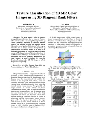
Fig. 2 shows the six diagonal x-y-z planes in a 3D
geometry.
YR YL ZR ZL XL XR
Fig. 2: Six diagonal planes in a 3D geometry
Table 1: Various diagonal planes
27-neighborhood
window
Diagonal
Planes
Vertices
of Planes
XL Plane
1,10,19,
5,14,23,
9,18,27
XR Plane
3,12,21,
5,14,23,
7,16,25
YL Plane
1,11,21,
4,14,24,
7,17,27
YR Plane
3,11,19,
6,14,22,
9,17,25
ZL Plane
1,2,3,
13,14,15,
25,26,27
ZR Plane
19,20,21,
13,14,15,
7,8,9

2. This paper introduces a technique for detecting
textures in all six x-y-z diagonal planes. In geometrical
terms, these diagonal planes are called “volumetric
features”.
II. PROPOSED METHOD
Apart from detecting latent textures in a given
image, one can also artificially create texture images.
Fig. 3 shows 3D texture images, which are artificially
generated using cellular automata rules.
(a) Image 1 (b) Image 2
Fig. 3: Texture images due to cellular automata rules
Texture detection in six diagonal x-y-z planes
To begin with, the directional texture detection
concept is explained with the help of planes
perpendicular to X, Y and Z axes. The given 3-D image
is plane-wise raster-scanned by the 27-neighborhood
window shown in Fig. 4. Now, the 3-D linear textures
are extracted along a desired axis with a directional
twist by choosing the plane which is perpendicular to
that axis and its associated rank of a particular
directional twist. Rank is decided by the reading
pattern. For instance, the Y-Z plane is perpendicular to
the X-axis and rank1 of zero directional twist denoted
by X1 is obtained by reading the values of the cells of
2,11,20,23,26,17,8,5 in the Y-Z central plane. Fig. 4
shows the Y-Z planes and their cell numbering.
Left plane Central plane Right plane
Fig. 4: Y-Z Planes perpendicular to X-axis
with cell numbering in 3x3x3 neighborhood
Processing is carried out using the values in the cells
and computed value placed in the central cell, that is, in
the 14th
cell. Texture detection algorithm is used for the
processing. Table 2 shows the reading patterns for
various ranks in terms of cell sequences
Table 2: Cell sequences for ranks in X, Y and Z axes
Axes Ranks Cell sequences
X
X1 2,11,20,23,26,17,8,5
X2 11,20,23,26,17,8,5,2
X3 20,23,26,17,8,5,2,11
X4 23,26,17,8,5,2,11,20
Y
Y1 4,5,6,15,24,23,22,13
Y2 5,6,15,24,23,22,13,4
Y3 6,15,24,23,22,13,4,5
Y4 15,24,23,22,13,4,5,6
Z
Z1 10,11,12,15,18,17,16,13
Z2 11,12,15,18,17,16,13,10
Z3 12,15,18,17,16,13,10,11
Z4 15,18,17,16,13,10,11,12
The Algorithm
On every move, sub image enclosed by the 3X3X3
window is inspected and the boundary values are stored
in an array according to the chosen cell sequence, that
is, the rank. For example, consider the reading sequence
2,11,20,23,26,17,8,5 corresponding to the X1 rank
filter. The configuration of rank X1 is denoted as the
number sequence c2,c11,c20,c23,c26,c17,c8,c5. The central
cell value is denoted as c14. Now all boundary cell
values ci (i=2,11,20,23,26,17,8,5) are compared with
c14. If ci c14 then the value of ci is made 1, else 0. Now
the computed configuration c2,c11,c20,c23,c26,c17,c8,c5 is a
binary valued string. The decimal equivalent of this
string is calculated and the resulting decimal value is
assigned to the central cell c14. This procedure is
repeated until entire image is scanned. The overall
effect is that all textures present in the given image in
the chosen axis are detected. There are a total of 36
rank filters, 12 in the X, Y, Z axes and 24 in XL, XR,
YL, YR, ZL and ZR axes. Table 3 presents 24 rank
filter cell sequences in XL, XR, YL, YR, ZL, ZR axes.
Table 3: Cell sequences in six diagonal axes
Axes Ranks Cell sequences
XL
XL1 1,10,19,23,27,18,9,5
XL2 10,19,23,27,18,9,5,1
XL3 19,23,27,18,9,5,1,10
XL4 23,27,18,9,5,1,10,19
XR
XR1 3,12,21,23,25,16,7,5
XR2 12,21,23,25,16,7,5,3
XR3 21,23,25,16,7,5,3,12
XR4 23,25,16,7,5,3,12,21
YL
YL1 1,11,21,24,27,17,7,4
YL2 11,21,24,27,17,7,4,1
YL3 21,24,27,17,7,4,1,11
YL4 24,27,17,7,4,1,11,21
YR
YR1 3,11,19,22,25,17,9,6
YR2 11,19,22,25,17,9,6,3
YR3 19,22,25,17,9,6,3,11
YR4 22,25,17,9,6,3,11,19
ZL ZL1 1,13,25,26,27,15,3,2

3. ZL2 13,25,26,27,15,3,2,1
ZL3 25,26,27,15,3,2,1,13
ZL4 26,27,15,3,2,1,13,25
ZR
ZR1 7,13,19,20,21,15,9,8
ZR2 13,19,20,21,15,9,8,7
ZR3 19,20,21,15,9,8,7,13
ZR4 20,21,15,9,8,7,13,19
The Pseudocode [ ]
3-D Directional Texture Detection
Input: 3-D image, threshold
Output: 3-D Direction Textures
Steps:
• Step 1: Read 3-D data and place voxel
values in input_array.
• Step 2: Copy contents of input_array to
another output_array
• Step 3: Repeat sliding the chosen plane
over the image; read values (input_array)
{
Step 3(a): If Pi >=P9 then Pi=1 else
Pi=0
Step 3(b): Place decimal equivalent
(boundary values of central voxel)
of binary values in the central
voxel(write in output_array)
}
Until the structuring element periods
whole of the image
• Step 4: Pass the output_array to
VolumeRenderer() method
As an example, consider XL plane and rank XL1. The
values in the cells 1,10,19,23,27,18,9,5 are read. Apply
the algorithm and evaluate the decimal value
corresponding to the texture and place the decimal
value in central cell 14. The XL refers to the left cut
plane which is oblique to X axis by 45 degrees. Fig. 5
shows the planar view of this surface.
Fig. 5: XL plane perpendicular to X-axis
and tilted by 45 degrees
XL2 allows the reading sequence 10,19,23,27,18,9,5,1
as shown in Fig. 5. After having chosen XL plane and
rank XL2, the 3-D image is scanned by the 3X3X3
window. As outlined earlier, sub image scanned by the
XL plane is inspected and the boundary values are
stored in an array according to the cell sequence
10,19,23,27,18,9,5,1, that is, the rank XL2. The texture
value is computed as per the algorithm and assigned to
the central cell 14. Fig. 6 shows texture patterns
extracted from image 2 using XL1 and XR1 rank filters.
Fig. 6 shows texture patterns extracted from image 2
using XL1 and XR1 rank filters. Fig. 7 shows texture
patterns extracted from image 2 using YL1 and YR1
rank filters. Fig. 8 shows texture patterns extracted from
image 2 using ZL1 and ZR1 rank filters.
Textures obtained using XL1 rank filter Textures obtained using XR1 rank filter
Fig. 6: Textures along XL and XR planes
Textures obtained using YL1 rank filter Textures obtained using YR1 rank filter
Fig. 7: Textures along YL and YR planes
Textures obtained using ZL1 rank filter Textures obtained using ZR1 rank filter
Fig. 8: Textures along ZL and ZR planes
The reading patterns for all 24 rank filters are given
in Figs. 9 to 20.
XL1=1,10,19,23,27,18,9,5 XL2=10,19,23,27,18,9,5,1
Fig. 9: Reading patterns for XL1 and XL2

4. XL3=19,23,27,18,9,5,1,10 XL4=23,27,18,9,5,1,10,19
Fig. 10: Reading patterns for XL3 and XL4
XR1=3,12,21,23,25,16,7,5 XR2=12,21,23,25,16,7,5,3
Fig. 11: Reading patterns for XR1 and XR2
XR3=21,23,25,16,7,5,3,12 XR4=23,25,16,7,5,3,12,21
Fig. 12: Reading patterns for XR3 and XR4
YL1=1,11,21,24,27,17,7,4 YL2=11,21,24,27,17,7,4,1
Fig. 13: Reading patterns for YL1 and YL2
YL3=21,24,27,17,7,4,1,11 YL4=24,27,17,7,4,1,11,21
Fig. 14: Reading patterns for YL3 and YL4
YR1=3,11,19,22,25,17,9,6 YR2=11,19,22,25,17,9,6,3
Fig. 15: Reading patterns for YR1 and YR2
YR3=19,22,25,17,9,6,3,11 YR4=22,25,17,9,6,3,11,19
Fig. 16: Reading patterns for YR3 and YR4
ZL1=1,13,25,26,27,15,3,2 ZL2=13,25,26,27,15,3,2,1
Fig. 17: Reading patterns for ZL1 and ZL2
ZL3=25,26,27,15,3,2,1,13 ZL4=26,27,15,3,2,1,13,25
Fig. 18: Reading patterns for ZL3 and ZL4
ZR1=7,13,19,20,21,15,9,8 ZR2=13,19,20,21,15,9,8,7
Fig. 19: Reading patterns for ZR1 and ZR2
ZR3=19,20,21,15,9,8,7,13 ZR4=20,21,15,9,8,7,13,19
Fig. 20: Reading patterns for ZR3 and ZR4

5. III. CASE STUDY
A sample MR image set called ‘toutaix” is
considered here for the case study. This image
corresponds to a human heart and is taken from the
website https://www.osirix-viewer.com/. MR images
are by default gray images. A coloring scheme has been
used to convert 3D gray images into 3D color images.
Details about this image are given in table 4
Table 4: Details of MR image ‘toutatix ‘
Website Details of the image Remarks
http://pubimage.
hcuge.ch:8080/
File name: Toutatix
Image type: MRI
Width = 256
Height = 256
Depth = 256
Max Gray level: 256
Reconstructed
from a set of
2-D slices
Fig. 21 shows MR image ‘toutatix’ and its colored
version. The color image voxels are depicted by R, G
and B values and the maximum value of a color
component is 255. Figs. 22 to 33 show the texture
detected versions of the color image ‘toutatix’ using all
24 rank filters.
All these 24 rank filters are defined in a
27-neighborhood structure shown on the
right. ATI Radeon HD R5970 Graphics
card has been used to process 3D images.
Fig. 21: Sample MRI image and its colored version
XL1 rank filtered XL2 rank filtered
Fig. 22: XL1 and XL2 rank filtered images
XL3 rank filtered XL4 rank filtered
Fig. 23: XL3 and XL4 rank filtered images
XR1 rank filtered XR2 rank filtered
Fig. 24: XR1 and XR2 rank filtered images
XR3 rank filtered XR4 rank filtered
Fig. 25: XR3 and XR4 rank filtered images
YL1 rank filtered YL2 rank filtered
Fig. 26: YL1 and YL2 rank filtered images
YL3 rank filtered YL4 rank filtered
Fig. 27: YL3 and YL4 rank filtered images
YR1 rank filtered YR2 rank filtered
Fig. 28: YR1 and YR2 rank filtered images
YR3 rank filtered YR4 rank filtered
Fig. 29: YR3 and YR4 rank filtered images

6. ZL1 rank filtered ZL2 rank filtered
Fig. 30: ZL1 and ZL2 rank filtered images
ZL3 rank filtered ZL4 rank filtered
Fig. 31: ZL3 and ZL4 rank filtered images
ZR1 rank filtered ZR2 rank filtered
Fig. 32: ZR1 and ZR2 rank filtered images
ZR3 rank filtered ZR4 rank filtered
Fig. 33: ZR3 and ZR4 rank filtered images
Observations
1. The rank filters XL1, XL2, XR1, XR2, YR3,
YR4, ZL1 and ZL2 extract texture regions
where the blood vessels are embedded.
2. The structure and form of the blood vessels
could be clearly seen in such filtered images.
IV. CONCLUSION
All 24 texture versions of the image obtained
using diagonal rank filters could be seen to provide a
concrete visual proof of the fact that textures in an
image are direction sensitive and so they could be used
for image segmentation purposes.
ACKNOWLEDGMENT
The authors thank the administration of Avatar
MedVision US LLC, NC, USA and Pentagram
Research Centre Private Limited, Hyderabad, India
various hospitals both in India and USA for providing
actual MR Images for the intended study. Technical
support from Mr. Srikanth Maddikunta and Mr. Rahul
Sharma of Pentagram Research Centre Pvt Ltd,
Hyderabad, India, is duly acknowledged. Further, we
acknowledge the permission given to us by the
management of Pentagram Research Centre Pvt. Ltd.,
to use the software “Logical 3D Image Processing
System (L3DIPS)” to implement some of our programs.
As a mark of our appreciation and gratitude, we show
below the screenshot image of the front-end of the
software L3DIPS.
REFERENCES
[1] Rajan E.G., “Symbolic computing: signal and image
processing”, Anshan Publications, Kent, United Kingdom,
2003.
[2] Rajan E. G., “Cellular logic array processing for high
through put image processing systems”, Sadhana, Vol. 18,
issue 2, pp. 279-300, Springer.
[3] Rajan E. G., “Fast algorithm for detecting volumetric and
superficial features in 3-D images”, International
Conference on Biomedical Engineering, Osmania
University, Hyderabad, 1994.
[4] Rajan E. G., “Medical imaging in the framework of
cellular logic array processing”, in Proc. 15th Annu. Conf.
Biomedical Society of India, Coimbatore Institute of
Technology, 1996.
[5] G. Ramesh Chandra, Towheed Sultana, G. Sathya,
“Algorithms for Generating Convex Polyhedrons In A
Three Dimensional Rectangular Array Of Cells”,
International Journal of Systemics, Cybernetics and
Informatics, April, 2011, pp 24-34.
[6] G. Ramesh Chandra, and E. G. Rajan, “Generation of Three
Dimensional Structuring elements over 3x3x3 Rectangular
Grid”, CIIT International Journal of Digital Image Proc.
Vol. 4, No.2, February 2012, pp.80-89.
[7] G. Ramesh Chandra and E. G. Rajan, “Algorithms for
generating convex polyhedrons over three dimensional
rectangular grid”; Signal & Image Processing : An
International Journal (SIPIJ), Vol.3, No.2, April 2012, pp.
197-206
[8] G. Ramesh Chandra and E. G. Rajan, “Algorithm for
Constructing Complete Distributive Lattice of Polyhedrons
Defined over Three Dimensional Rectangular Grid- Part II”;
CCSIT Conference, Bangalore, proceedings are published
by LNICST, Springer, pp. 202-208.