PSY325 Week 2 Scenario and Data Set 4 Source Adapted fr.docx

PSY325 Week 2 Scenario and Data Set 4
Source: Adapted from Tanner (2016, p. 320)
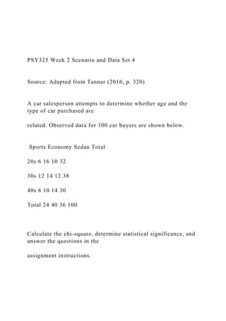
A car salesperson attempts to determine whether age and the
type of car purchased are
related. Observed data for 100 car buyers are shown below.
Sports Economy Sedan Total
20s 6 16 10 32
30s 12 14 12 38
40s 6 10 14 30
Total 24 40 36 100
Calculate the chi-square, determine statistical significance, and
answer the questions in the
assignment instructions.

Method Note
The Chi-Square Test:
Often Used and More Often
Misinterpreted
Todd Michael Franke
1
, Timothy Ho
2
, and
Christina A. Christie
3
Abstract
The examination of cross-classified category data is common in
evaluation and research, with Karl
Pearson’s family of chi-square tests representing one of the
most utilized statistical analyses for
answering questions about the association or difference between
categorical variables. Unfortu-
nately, these tests are also among the more commonly
misinterpreted statistical tests in the field.
The problem is not that researchers and evaluators misapply the
results of chi-square tests, but
rather they tend to over interpret or incorrectly interpret the
results, leading to statements that
may have limited or no statistical support based on the analyses
preformed.
This paper attempts to clarify any confusion about the uses and

interpretations of the family of
chi-square tests developed by Pearson, focusing primarily on
the chi-square tests of independence
and homogeneity of variance (identity of distributions). A brief
survey of the recent evaluation lit-
erature is presented to illustrate the prevalence of the chi-square
test and to offer examples of how
these tests are misinterpreted. While the omnibus form of all
three tests in the Karl Pearson family
of chi-square tests—independence, homogeneity, and goodness-
of-fit,—use essentially the same
formula, each of these three tests is, in fact, distinct with
specific hypotheses, sampling approaches,
interpretations, and options following rejection of the null
hypothesis. Finally, a little known option,
the use and interpretation of post hoc comparisons based on
Goodman’s procedure (Goodman,
1963) following the rejection of the chi-square test of
homogeneity, is described in detail.
Keywords
chi-square test, quantitative methods, methods use, using chi-
square test
1 Department of Social Welfare, Meyer and Rene Luskin School
of Public Affairs, University of California, Los Angeles, CA,
USA
2
Department of Education, Graduate School of Education and
Information Sciences, University of California, Los Angeles,
CA, USA
3
Department of Education, Social Research Methods Division,

Graduate School of Education and Information Sciences,
University of California, Los Angeles, CA, USA
Corresponding Author:
Todd Michael Franke, Department of Social Welfare, Meyer and
Rene Luskin School of Public Affairs, University of California,
Box 951656, Los Angeles, CA, 90095, USA
Email: [email protected]
American Journal of Evaluation
33(3) 448-458
ª The Author(s) 2012
Reprints and permission:
sagepub.com/journalsPermissions.nav
DOI: 10.1177/1098214011426594
http://aje.sagepub.com
Karl Pearson initially developed the chi-square test in 1900 and
applied it to test the goodness of fit
for frequency curves. Later, in 1904, he extended it to
contingency tables to test for independence
between rows and columns (Stigler, 1999). Since then, the
Pearson family of chi-square tests has
become one of the most common sets of statistical analyses in
evaluation and social science
research. Unfortunately, these tests are also among the more
commonly misinterpreted statistical

tests in the field. The problem is not that researchers and
evaluators misapply the results of chi-
square tests, but rather they tend to over interpret or incorrectly
interpret the results, leading them
to make statements that may have limited or no statistical
support based on the analyses preformed.
In this article, we will attempt to clarify any confusion about
the uses and interpretations of the
family of chi-square tests developed by Pearson, focusing
primarily on the chi-square tests of inde-
pendence and homogeneity of variance (identity of
distributions). First, the family of chi-square sta-
tistics will be presented, including distinguishing features of
and appropriate uses for each specific
test. Next, a brief survey of the recent evaluation literature will
be presented to illustrate the preva-
lence of the chi-square test and to offer examples of how these
tests are misinterpreted. Finally, a
little known option, the use of post hoc comparisons based on
Goodman’s procedure (Goodman,
1963) following the rejection of the chi-square test of
homogeneity, will be described.
The Karl Pearson Family of Chi-Square Tests

The chi-square test is computationally simple. It is used to
examine independence across
two categorical variables or to assess how well a sample fits the
distribution of a known population
(goodness of fit). The chi-square tests in the Karl Pearson
family are not to be confused with others
such as the Yates chi-square test (correction for continuity), the
Mantel–Haenszel chi-square or the
Maxwell–Stuart tests of correlated proportions. Each of these
has its own applications, though they
all utilize the chi-square distribution as the reference
distribution. In fact, many tests that assess
model fit use the chi-square distribution as the reference
distribution. For example, many covar-
iance structure analyses, including factor analysis and structural
equation modeling, assess model
fit by comparing the sample covariances to those derived from
the model. Again, while they are
based on the same chi-square distribution, these tests are similar
to the Karl Pearson family of tests
only in that they compare an observed set of data to what is
expected.
The omnibus form of all three tests in the Karl Pearson family
of chi-square tests—goodness of

fit, independence, homogeneity—use essentially the same
formula. Each of these three tests is, in
fact, distinct with specific hypotheses, interpretations, and
options following rejection of the null
hypothesis. The formula for computing the test statistic is as
follows:
w2 ¼
Xn
i¼1
ðOi � EiÞ2
Ei
;
where n is the number of cells in the table. The obtained test
statistic is compared against a critical
value from the chi-square distribution with (r � 1)(c � 1)
degrees of freedom.
The main difference across each of the three chi-square tests
relates to the appropriate situations
for which each should be used. The chi-square goodness of fit
test is used when a sample is com-
pared on a variable of interest against a population with known
parameters. For example, a goodness
of fit test might be applied on a survey sample to compare
whether the ethnicity or income of the
survey respondents is consistent with the known demographic

makeup of the geographic locale from
which the sample was drawn. The null and alternative
hypotheses are:
Hypothesis0: The data follow a specified distribution.
HypothesisA: The data do not follow the specified distribution.
Franke et al. 449
The interpretation upon rejection is that the sample differs
significantly from the population on
the variable of interest.
The chi-square test of independence determines whether two
categorical variables in a single
sample are independent from or associated with each other. For
example, a survey might be admi-
nistered to 1,000 participants who each respond with their hair
color and favorite ice cream flavor.
The test would then be used to determine whether hair color and
ice cream preference are indepen-
dent of each other. The null and alternative hypotheses are as
follows:
Hypothesis0: The variables of interest are independent.
HypothesisA: The variables of interest are associated.

A significant test rejecting the null hypothesis would suggest
that within the sample, one variable
of interest is associated with a second variable of interest.
Finally, the chi-square test of homogeneity is used to determine
whether two or more independent
samples differ in their distributions on a single variable of
interest. One common use of this test is to
compare two or more groups or conditions on a categorical
outcome. A significant test statistic
would indicate that the groups differ on the distribution of the
variable of interest but does not indi-
cate which of the groups are different or where the groups
differ. The null and alternative hypotheses
are as follows:
Hypothesis0: The proportions between groups are the same.
HypothesisA: The proportions between groups are different.
We focus on the practical and important differences between the
tests of independence
and homogeneity because they are so frequently used in
evaluation and applied research studies.
Despite the fact that the formulation of the omnibus test
statistic is the same for the test of inde-

pendence and the test of homogeneity, these two tests differ in
their sampling assumptions, null
hypotheses, and options following a rejection. The main
difference between them is how data are
collected and sampled. Specifically, the test of independence
collects data on a single sample, and
then compares two variables within that sample to determine the
relationship between them. The
test of homogeneity collects data on two
1
or more distinct groups intentionally, as might be the
case in a treatment or intervention study with a comparison
group. The two samples are then com-
pared on a single variable of interest to test whether the
proportions differ between them. Wickens
(1989) presents a thoughtful and succinct description of these
tests, as well as their sampling
assumptions and hypotheses. In addition to the tests of
homogeneity and independence, Wickens
presents an additional alternative where both margins are fixed,
which he refers to as ‘‘test of unre-
lated classification.’’
When data are collected using only a single sample, only the
test of independence is valid and

only interpretations of association between variables can be
made. When data on two or more sam-
ples are collected, the test of homogeneity is appropriate and
comparisons of proportions can be
made across the multiple groups. When sampling occurs from
multiple populations, and thus the
homogeneity hypothesis appropriate, it is also reasonable
(although less interesting) to ask the inde-
pendence question.
In the above example regarding hair color and ice cream
preference, if the researcher
defined the population by hair color and eye color and collected
information on 500
brunettes and 500 blondes, these would constitute two
independent samples. Comparisons of
proportions of blondes and brunettes by their ice cream
preferences would be valid. When
random assignment is used to assign participants to two or more
conditions, these groups are
by definition independent and the test of homogeneity may be
used to test for differences
between the groups.
450 American Journal of Evaluation 33(3)

Perhaps, these distinctions can be best illustrated by the null
hypothesis tested in each of
these two tests. The chi-square test of independence null
hypothesis states no association
between two categorical variables. It can be written as H0 : f ¼
0 or H0 : n ¼ 0. This states
that the association between two categorical variables, as
measured by a Phi (f) correlation
for 2 � 2 contingency tables or with Kramer’s V for larger
tables, is zero or the variables are
independent.
H0 : f ¼ 0
HA : f 6¼ 0
or
H 0 : V ¼ 0;
H A : V 6¼ 0:
The chi-square test of homogeneity compares the proportions
between groups on a variable of
interest. The null hypothesis is presented in matrix form:
H0 :¼
p11 ¼ p12 ¼ ::: ¼ p1k
p21 ¼ p22 ¼ ::: ¼ p2k
p31 ¼ p32 ¼ ::: ¼ p3k
pk1 ¼ pk2 ¼ ::: ¼ pkk

2
6664
3
7775
HA : The null is false
Rejection of the null hypothesis in the case of three or more
groups only allows the researcher to
conclude that the proportions between the groups differ, not
which groups are different. Table 1
summarizes the distinction between the three types of chi-
square tests—specifically, the sampling
required for each test, the correct interpretation of each test,
and the null hypothesis assumed of
each test.
One common misinterpretation of chi-square tests comes from
not distinguishing between these
three specific tests. Indeed, when most researchers declare that
they ‘‘utilized a chi-square test,’’
they are typically referring to the chi-square test of
independence. This lack of specificity often leads
researchers to use interpretations of one test where another was
actually conducted. For example,
researchers will more often feel compelled to compare the
proportions between groups, regardless

of how the data were drawn. As is most often the case, the data
on two categorical variables are
collected from a single sample (e.g., survey data), where the
assumptions for chi-square test of
homogeneity are not met, and an interpretation comparing
proportions between groups is not valid.
Even in those situations where data are drawn from multiple
samples and the test of homogeneity
is appropriate, researchers seem unaware that procedures exist
to specifically follow-up after the
rejection of the omnibus test. Consider the following null
hypothesis:
H0 :
p11 ¼ p12 ¼ p13
p21 ¼ p22 ¼ p23
� �
:
Table 1. Chi-Square Tests and Attributes
Chi-Square Test
Attribute Test of Independence Test of Homogeneity Test of
Goodness of Fit
Sampling type Single dependent sample Two (or more)
independent samples
Sample from population

Interpretation Association between variables Difference in
proportions Difference from population
Null hypothesis No association between
variables
No difference in
proportion between
groups
No difference in distribution
between sample and
population
Franke et al. 451
A rejection in this case indicates that at least one proportion is
different from at least one other
proportion.
2
Often, a researcher will conduct a chi-square test, find a
significant value, and then look
for the cells with the largest disparity in proportions or
frequencies to make a substantive interpreta-
tion. The proper procedure would involve conducting post hoc
comparisons after the omnibus
chi-square test to determine where the significant differences
actually are. Post hoc procedures for

chi-square tests are discussed in a later section.
Chi-square Tests in Recent Evaluation Literature
A brief survey of recent evaluation literature was conducted in
order to obtain a general sense of how
often chi-square tests are used and how often researchers
misinterpret the results.
Surveying the evaluation literature is an approach that has been
used by several researchers as a
method for better understanding the methods and strategies used
in evaluation practice. For example,
Greene, Caracelli, and Graham (1989) included published
evaluation studies in their sample when
reviewing 57 empirical mixed-methods evaluations. Findings
from the empirical study were used to
refine a mixed-methods conceptual framework that had
originally been developed from the theore-
tical literature and was intended to inform and guide practice.
More recently, Miller and Campbell
(2006) studied empowerment evaluation in practice by
examining 47 case examples published from
1994 through June 2005 to determine the extent to which
empowerment evaluation could be distin-
guished from evaluation approaches emphasizing similar

elements, and the extent to which empow-
erment evaluation led to empowered outcomes for program
beneficiaries.
For the current study, four prominent evaluation journals were
selected for review: American
Journal of Evaluation, Evaluation Review, Educational
Evaluation and Policy Analysis, and Eva-
luation and Program Planning. Every article published in these
four journals between January
2008 and August 2010 was reviewed. These journals and
periods were not intended to be a compre-
hensive search of the evaluation literature, but mainly to obtain
a picture of the prevalence of
chi-square tests and the extent to which these tests are
incorrectly interpreted. The vast majority
of chi-square tests and misinterpretations probably exist in
evaluation reports that are never read
beyond a small circle of intended users, but we believe that the
proliferation of chi-square test mis-
interpretations is exacerbated by evaluation literature that is
read by a larger audience.
After book reviews, section introductions, memoranda, and
other editorial content were excluded,
there were a total of 292 articles available for review. Two

graduate student researchers coded each
article on a variety of measures, including whether inferential
statistics were used and whether a chi-
square test was used. For articles that used a chi-square test,
additional codes identified whether the
article contained the correct interpretation given the sampling
procedure, whether post hoc interpre-
tations were used, and whether post hoc tests were conducted.
Table 2 details the number of articles in each journal as well as
how many used inferential
quantitative statistics. Overall, just over a third (36.6%; n ¼
107) of the articles used some sort
Table 2. Use of Statistical Tests in Journal Articles
Total
Number
of Articles
Articles Using
Inferential
Statistics
Articles Using
Chi- Square
Test
Proportion of

Articles Using
Chi-Square Test (%)
American Journal of Evaluation 65 16 3 18.75
Evaluation Review 61 30 11 36.67
Educational Evaluation and Policy Analysis 52 35 6 17.14
Evaluation and Program Planning 114 26 12 46.15
Total 292 107 32 29.91
of inferential statistic, ranging from a simple t test to more
advanced structural equation models. Of
the 107 articles that used inferential statistics, 32 articles
(29.9%) also used a chi-square test in the
Karl Pearson family. Evaluation and Program Planning had the
most articles employing a chi-
square test (n ¼ 12) while the American Journal of Evaluation
had the fewest (n ¼ 3).
The 32 articles that used chi-square tests were further reviewed
to determine whether the inter-
pretations were justified. Often, researchers were not specific
about which chi-square tests were
being used (only one of the 32 articles correctly specified the
type of chi-square test conducted).
To make the determination, then, coders reviewed the Method
section in each article to identify

which chi-square test would have been appropriate given the
sampling design used. The interpreta-
tions from the chi-square tests presented in each article were
then coded for the types of interpreta-
tion used, that is, whether an association claim was made
between variables or whether a comparison
of proportions was made between groups. This allowed the
researchers to determine the type of
chi-square test used by the researchers in each article. Any
discrepancy between a study’s sampling
design and the type of chi-square test used was coded as a
nonvalid interpretation of the chi-
square test. In addition, each of the 32 chi-square articles was
coded on whether a post hoc inter-
pretation was used, meaning that the author made comparisons
across select rows and columns of
the table.
The results from these additional analyses are presented in
Table 3. Overall, less than half of
the chi-square articles (43.75%; n ¼ 14) had interpretations that
were justified by the type of
chi-square test used. All three articles in the American Journal
of Evaluation included the correct
usage of the chi-square test, whereas only a third (two out of
six) of the articles in Educational

Evaluation and Policy Analysis did so. As shown in Table 3, 9
of the 32 articles that used chi-
square (28.1%) included a post hoc interpretation. None of the
articles used any post hoc analyses
to justify their claims.
Hypothetical Example: Support Components for At-Risk
Families
We offer a hypothetical example to illustrate the concepts
described above and to guide readers
through a proper chi-square post hoc analysis. In this scenario,
suppose that researchers are inves-
tigating the impact of various family support components for
families at risk for child abuse and
neglect. Study participants were randomly assigned to receive
either parent education/life skills,
connections to community resources, or wraparound services
made up of the previous components
plus case management. Using the county data system, a sample
was drawn from each of these three
conditions. The dependent variable of interest consisted of 4
outcomes measures 12 months after the
families’ initial involvement with Child Protective Services
(CPS): (a) a CPS rereferral; (b) a sub-
stantiated allegation; (c) the child’s removal from home; or (d)

no further involvement with CPS.
Table 3. Description of Articles Using Chi-Square Analyses
Number of
Chi-Square
Articles
Number of Articles that
Used a Valid Chi-Square
Test Interpretation
Number of Articles
that Used a Post
Hoc Interpretation
N N % N %
American Journal of Evaluation 3 3 100.00 1 33.33
Evaluation Review 11 4 36.36 4 36.36
Educational Evaluation and Policy Analysis 6 2 33.33 2 33.33
Evaluation and Program Planning 12 5 41.67 2 16.67
Total 32 14 43.75 9 28.13
Franke et al. 453
While randomization is often used to form independent groups,
it is not a prerequisite for the appro-
priate use of the test for homogeneity. What is required is that
the groups are identified and sampled

intentionally. Table 4 shows the distribution with involvement
with CPS across the three conditions.
The null hypothesis is as follows:
H0 :
p11 ¼
p21 ¼
p31 ¼
p41 ¼
p12 ¼
p22 ¼
p32 ¼
p42 ¼
p13
p23
p33
p43
2
6664
3
7775;
HA : The null is false:
The obtained X 26 ¼ 36:77 is significant at the conventional a
level of .05. The justified interpre-

tation following the rejection of the null hypothesis would be to
conclude that the proportions are not
equal across the three groups.
Often at this point, researchers will conclude that the
proportions are not equal and will want
to compare specific conditions. For example, they might
examine the ‘‘no new involvement’’
row and conclude that the wraparound condition (72.3%) is
preferable to the parent education
(52.2%) or community resources (63.8%) condition.
Alternatively, a researcher may be inter-
ested in comparing the proportion of children removed across
the conditions. It might be tempt-
ing to conclude that parent education (14.5%) is significantly
different from community
resources (4.26%) and wraparound (4.2%). However, this
interpretation would be incorrect
because there is no statistical justification for these claims
based solely on the results of the
omnibus test; the omnibus test indicates only that the conditions
are significantly different but
not which conditions are different.
Because the chi-square test is an omnibus test, post hoc
procedures would need to be con-
ducted in order to compare individual conditions. As previously
mentioned, the procedure for

comparing conditions or groups was developed by Goodman
(1963).
3
Similar to the comparison
procedures following an analysis of variance (ANOVA), several
different approaches—includ-
ing Scheffé, Holm,
4
and Dunn-Bonferroni—are available for selecting the
appropriate critical
value. Also similar to the ANOVA, the comparison often takes
on the name associated with
formulation of the critical value. For purposes of this article,
the Scheffé post hoc values are
presented because this represents the most conservative
approach. For an alternative approach
based on Dunn-Bonferonni, see Marasculio and Serlin (1988).
The Goodman procedure is described below. The test statistic
for each contrast is as follows:
ĉffiffiffiffiffiffiffiffi
SE2c
q ¼ Z:
Table 4. Involvement with CPS and Service Conditions

Parent Education Community Resources Wraparound Total
N, Col % N, Col % N, Col % N, Col %
Rereferral to CPS 38, 20.43 42, 22.34 49, 13.73 129, 17.65
Substantiated allegation 24, 12.9 18, 9.57 35, 9.8 77, 10.53
Child removed 27, 14.52 8, 4.26 15, 4.2 50, 6.84
No new involvement with CPS 97, 52.15 120, 63.83 258, 72.27
475, 64.98
Total 186 188 357 731
Note. CPS ¼ child protective services.
The same equation in an expanded form is as follows:
ĉffiffiffiffiffiffiffiffi
SE2c
q ¼ w1ðp1Þ�
w2ðp2Þffiffiffiffiffiffiffiffiffiffiffiffiffiffiffiffiffiffiffiffiffiffiffi
ffiffiffiffiffiffiffiffiffiffiffiffiffiffiffiffiffiffiffiffiffiffiffiffiffi
w21
p1q1
n1
� �
þ w22
p2q2
n2

� �s ¼ Z;
where ĉ represents the linear combination of weights (Wk) and
proportions (yk ) of the specific
contrast:
c ¼ W1y1 þ W2y2 þ�� þ Wkyk;
where
W1 þ W2 þ�� þ Wk ¼ 0:
And the numerator of the test is the square root of the weighted
standard error of the contrast:
SE
2
c ¼ W
2
1 SE
2
y1
þ W 22 SE
2
y2
þ�� þ W 2k SE
2
yk
:
The standard error of each column is the standard error of an
estimated proportion:

SE
2
y ¼
pk qk
Nk
:
Once the obtained test statistic is found for a comparison of
interest, it is compared to a critical
value. The Scheffé critical value is found by taking the square
root of the critical value in the original
omnibus chi-square analysis. In the above example, the chi-
square omnibus critical value at the con-
ventional a level of .05 with (r � 1)(c � 1) ¼ (4 � 1)(3 � 1) ¼
6 degrees of freedom is 12.59. The
square root of this critical value is S� ¼
ffiffiffiffiffiffiffiffiffiffiffiffi
w2v:1�a
p
¼
ffiffiffiffiffiffiffiffiffiffiffi
12:59
p
¼�3:55 which represents the Scheffé
critical value for all contrasts.

Referring back to our previous example, comparing wraparound
(72.3%) to parent education
(52.2%) on ‘‘no new involvement’’ leads to the following
hypothesis:
Hypothesis0 : pNo new involvement=wraparound ¼ pNo new
involvement=parent education;
HypothesisA : pNo new involvement=wraparound 6¼ pNo new
involvement=parent education:
The appropriate test statistic is as follows:
357
357
� �
:7227ð Þ�
186
186
� �
:5215ð
Þffiffiffiffiffiffiffiffiffiffiffiffiffiffiffiffiffiffiffiffiffiffiffiffiffiff
iffiffiffiffiffiffiffiffiffiffiffiffiffiffiffiffiffiffiffiffiffiffiffiffiffiffi
ffiffiffiffiffiffiffiffiffiffiffiffiffiffiffiffiffiffiffiffiffiffiffiffiffiffi
ffiffiffiffiffiffiffi
357
357
� �2

:7227ð Þ :2773ð Þ
357
� �
þ
186
186
� �2
:5215ð Þ :4785ð Þ
186
� �s ¼ :2012:0436 ¼ 4:61:
Since this is a pairwise comparison, the weights
357
357
and
186
186
equal 1, and essentially dropout of
the equation both in the numerator and in the denominator.
Given 4.61 > +3.55, we reject and con-
clude that there is a statistically significant difference between
these conditions.
Comparisons can be performed within any row. If the researcher
wanted to compare wraparound

(4.2%) to parent education (14.5%) on whether a child was
removed, ‘‘child removed,’’ the test sta-
tistic is given by
Franke et al. 455
357
357
� �
:042ð Þ�
186
186
� �
:1452ð
Þffiffiffiffiffiffiffiffiffiffiffiffiffiffiffiffiffiffiffiffiffiffiffiffiffiff
iffiffiffiffiffiffiffiffiffiffiffiffiffiffiffiffiffiffiffiffiffiffiffiffiffiffi
ffiffiffiffiffiffi
357
357
� ��
:042ð Þ :958ð Þ
357

� �
þ
186
186
� �
:1452ð Þ :8548ð Þ
186
� �s ¼�:1031:0278 ¼�3:69:
Given �3.69 > +3.55, we reject and conclude that there is a
statistically significant difference
between these conditions. A comparison between community
resources (4.26%) and parent educa-
tion (14.5%) produces a test statistic of 3.45 and is not
significant due to the differing sample sizes
and their impact on the standard error. This is an instance where
simply examining the difference
between the proportions, without conducting the appropriate
post hoc test, might lead to a statisti-
cally unsupported conclusion. In both of these, the comparisons
the difference between the parent
education and the other two conditions were .10. However, in
one case, there was a significant dif-
ference and in the other there was no difference based on the
critical value. A complete listing of all

pairwise comparisons is available in the Table 5 at the end of
article.
As noted previously, comparisons under this model are not
limited to being pairwise. The post
hoc procedure can also be used to test complex contrasts.
Suppose you want to compare wraparound
to the combination of parent education and community
resources.
357
357
� �
:1373ð Þ�
186
374
� �
:2043ð Þþ
188
374
� �
:2234ð Þ
� �

ffiffiffiffiffiffiffiffiffiffiffiffiffiffiffiffiffiffiffi
357
357
� �2
:1373ð Þ :8657ð Þ
357
� �
þ
186
374
� �2
:2043ð Þ :7957ð Þ
186
� �
þ
188
374
� �2
:2234ð Þ :7766ð Þ

188
� �" #vuut
¼
�:0766
:0273
¼�2:81:
Unlike with the previous pairwise contrast weights, the
combination of parent education and
community resources needs to be weighted for their respective
contributions. Once this is done, the
Table 5. Pairwise Contrasts from Hypothetical Example
c SE TS
Rereferral
Wraparound versus parent education �.0670 .0347 �1.931
Wraparound versus community resources �.0861 .0354 �2.432
Parent education versus community resources �.0191 .0424
�0.451
Substantiated abuse
Wraparound versus community resources .0023 .0306 0.075
Parent education versus community resources .0333 .0326 1.020
Child removed
Wraparound versus community resources �.0005 .0182 �0.030
Parent education versus community resources .1026 .0297 3.451

No new case opened
Wraparound versus parent education .2012 .0436 4.612
Wraparound versus community resources .0844 .0423 1.995
Parent Education versus community resources �.1168 .0507
�2.304
test statistic is calculated as it was before. Given �2.81 <
+3.55, we do not reject and conclude that
there is not a statistically significant difference between the
wraparound condition and the combi-
nation of parent education and community resources.
Discussion
Common misconceptions of the chi-square test were clarified in
this article. Specifically, we have
distinguished between the members of the Karl Pearson family
of chi-square tests and presented post
hoc procedures. Evaluators often need to examine the
association between categorical variables or to
compare groups or conditions on a categorical outcome, which
explains their prevalence in evalua-
tion literature and reports. However, effective use of the chi-
square test, or any other statistical test
for that matter, is dependent on a clear understanding of the

assumptions of the test and what is actu-
ally being tested (null hypothesis) in the statistical procedure.
A correct interpretation of the chi-square test or of other
statistical procedures is often dependent
on factors outside of distributional assumptions and
characteristics of the data itself—for example,
individual observations must be independent from other
observations in the contingency table. When
this is this case, an interpretation of the chi-square test is based
on sampling procedures and how data
were collected. Furthermore, since the asymptotic
approximation of the chi-square test is less precise
at the extreme end of the distribution, expected values of cells
need to be greater than five.
The review of the evaluation literature reveals that in about half
of the instances where a chi-square test
was used, the wrong interpretation was presented. The
appropriate interpretation of the results is directly
tied to the null hypothesis under test and the interpretation—
whether independence or homogeneity—is
limited to that hypothesis. More commonly, researchers prefer
to interpret the chi-square test of homo-
geneity by comparing groups across a variable of interest.
However, the sampling procedure precludes the

researcher from making this claim and has thus misinterpreted
the results of the chi-square test.
Researchers also tend to over interpret the results of statistical
tests. An omnibus chi-square test
informs us that the distribution of observed values deviates
from expected values, but does not tell us
where the discrepancy is located in the contingency table.
Often, researchers will make naı̈ ve com-
parisons between two or more groups without conducting any
post hoc tests to determine whether
the contrasts were significant.
Many more complex statistical models exist and we have faith
that these procedures are still being
faithfully and thoughtfully applied. Although the chi-square
tests were found to be commonly misinter-
preted in recent evaluation literature, the results of these studies
are not wrong. Rather, the problem is
simply that there is often no statistical justification for some of
the claims being made. However, Good-
man’s procedure is computationally simple and there is little
reason it cannot be conducted to justify
significant contrasts. Our hope in this article is that researchers
and evaluators will be more thoughtful

in using common statistical procedures and more carefully
consider what their results actually say.
Declaration of Conflicting Interests
The author(s) declared no potential conflicts of interest with
respect to the research, authorship, and/or publication
of this article.
Funding
The author(s) received no financial support for the research,
authorship, and/or publication of this article.
Notes
1. The two-sample test of proportions, which uses the Z
distribution, is a special case of the test of homoge-
neity, employed when you have only two groups.
Franke et al. 457
2. Comparisons in this context are limited to pairwise contrasts.
It is perfectly feasible that Groups 2 and 3
combined are from Group 1 and responsible for the significant
result.
3. The approach presented here builds logically on the post hoc
procedures following multiple group compar-
isons in analysis of variance (ANOVA) models. Goodman’s

approach is not the only one available for
addressing pairwise comparisons, however. See Seaman and
Hill (1996), Gardner (2000), and Delucchi
(1993).
4. Information on the use of the Holm procedure, see Holm,
1979.
References
Delucchi, K. L. (1993). On the use and misuse of chi-square. In
G. Keren & C. Lewis (Eds.), A handbook for
data analysis in the behavioral sciences (pp. 295–319).
Hillsdale, NJ: Lawrence Erlbaum.
Gardner, R. C. (2000). Psychological statistics using SPSS for
Windows. Upper Saddle River, NJ: Prentice Hall.
Greene, J. C., Caracelli, V. J., & Graham, W. F. (1989). Toward
a conceptual framework for mixed-method
evaluation designs. Educational Evaluation and Policy Analysis,
11, 255–274.
Goodman, L. (1963). Simultaneous confidence intervals for
contrasts among multinomial populations. The
Annals of Mathematical Statistics, 35, 716–725.
Holm, S. (1979). A simple sequentially rejective multiple test
procedure. Scandinavian Journal of Statistics, 6,
65–70.

Marasculio, L., & Serlin, R. (1988). Statistical methods for the
social and behavioral sciences. New York, NY:
W.H. Freeman.
Miller, R. L., & Campbell, R. (2006). Taking stock of
empowerment evaluation: An empirical review. American
Journal of Evaluation, 27, 296–319.
doi:10.1177/109821400602700303
Seaman, M. H., & Hill, C. C. (1996). Pairwise comparisons for
proportions: A note on Cox and Key. Educational
and Psychological Measurement, 56, 452–459.
Stigler, S. (1999). Statistics on the table: The history of
statistical concepts and methods. Cambridge, MA:
Harvard University Press.
Wickens, T. D. (1989). Multiple contingency tables analysis for
the social sciences. Hillsdale, NJ: Lawrence
Erlbaum.
Lessons in biostatistics
The Chi-square test of independence

Mary L McHugh
Department of Nursing, School of Health and Human Services,
National University, Aero Court, San Diego, California, USA
Corresponding author: [email protected]
Abstract
The Chi-square statistic is a non-parametric (distribution free)
tool designed to analyze group differences when the dependent
variable is measured
at a nominal level. Like all non-parametric statistics, the Chi-
square is robust with respect to the distribution ofthe data.
Specifically, it does not
require equality of variances among the study groups or
homoscedasticity in the data. It permits evaluation of both
dichotomous independent va-
riables, and of multiple group studies. Unlike many other non-
parametric and some parametric statistics, the calculations
needed to compute the
Chi-square provide considerable information about how each of
the groups performed in the study. This richness of detail allows
the researcher to
understand the results and thus to derive more detailed
information from this statistic than from many others.
The Chi-square is a significance statistic, and should be
followed with a strength statistic. The Cramer's V is the most
common strength test used
to test the data when a significant Chi-square result has been
obtained. Advantages of the Chi-square include its robustness
with respect to dis-
tribution of the data, its ease of computation, the detailed
information that can be derived from the test, its use in studies
for which parametric
assumptions cannot be met, and its flexibility in handling data

from both two group and multiple group studies. Limitations
include its sample size
requirements, difficulty of interpretation when there are large
numbers of categories (20 or more) in the independent or
dependent variables, and
tendency ofthe Cramer's V to produce relative low correlation
measures, even for highly significant results.
Key words: Chi-square; non-parametric; assumptions;
categorical data; statistical analysis
Received: April 1,2013 Accepted: May 6,2013
Introduction
The Chi-square test of independence (also known
as the Pearson Chi-square test, or simply the Chi-
square) is one ofthe most useful statistics for test-
ing hypotheses when the variables are nominal, as
often happens in clinical research. Unlike most sta-
tistics, the Chi-square (x )̂ can provide information
not only on the significance of any observed dif-
ferences, but also provides detailed information
on exactly which categories account for any differ-
ences found. Thus, the amount and detail of infor-
mation this statistic can provide renders it one of
the most useful tools in the researcher's array of
available analysis tools. As with any statistic, there
httpJ/dx.doi.org/10.11613/BM.2013.018
are requirements for its appropriate use, which are
called "assumptions" of the statistic. Additionally,
the x^ is a significance test, and should always be
coupled with an appropriate test of strength.

The Chi-square test is a non-parametric statistic,
also called a distribution free test. Non-parametric
tests should be used when any one of the follow-
ing conditions pertains to the data:
1. The level of measurement of all the variables is
nominal or ordinal.
2. The sample sizes of the study groups are un-
equal; for the x^ the groups may be of equal
size or unequal size whereas some parametric
tests require groups of equal or approximately
equal size.
3. The original data were measured at an interval
or ratio level, but violate one of the following
assumptions of a parametric test:
Biochemia Medica 2013;23(2):143-9
143
McHughML Chi-square
a) The distribution of the data was seriously
skewed or kurtotic (parametric tests assume
approximately normal distribution of the de-
pendent variable), and thus the researcher
must use a distribution free statistic rather than
a parametric statistic.
b) The data violate the assumptions of equal vari-
ance or homoscedasticity.

c) For any of a number of reasons (1), the continu-
ous data were collapsed into a small number of
categories, and thus the data are no longer in-
terval or ratio.
Assumptions of the Chi-square
As with parametric tests, the non-parametric tests,
including the x^ assume the data were obtained
through random selection. However, it is not un-
common to find inferential statistics used when
data are from convenience samples rather than
random samples. (To have confidence in the re-
sults when the random sampling assumption is vi-
olated, several replication studies should be per-
formed with essentially the same result obtained).
Each non-parametric test has its own specific as-
sumptions as well. The assumptions of the Chi-
square include:
1) The data in the cells should be frequencies,
or counts of cases rather than percentages or
some other transformation of the data.
2) The levels (or categories) of the variables are
mutually exclusive. That is, a particular subject
fits into one and only one level of each of the
variables.
3) Each subject may contribute data to one and
only one cell in the x -̂ If, for example, the same
subjects are tested over time such that the
comparisons are of the same subjects at Time 1,
Time 2, Time 3, etc., then x^ may not be used.
4) The study groups must be independent. This

means that a different test must be used if the
two groups are related. For example, a differ-
ent test must be used if the researcher's data
consists of paired samples, such as in studies in
which a parent is paired with his or her child.
5) There are 2 variables, and both are measured
as categories, usually at the nominal level. How-
ever, data may be ordinal data. Interval or ratio
data that have been collapsed into ordinal cat-
egories may also be used. While Chi-square has
no rule about limiting the number of cells (by
limiting the number of categories for each vari-
able), a very large number of cells (over 20) can
make it difficult to meet assumption #6 below,
and to interpret the meaning of the results.
6) The value of the cell expecteds should be 5 or
more in at least 80% of the cells, and no cell
should have an expected of less than one (3).
This assumption is most likely to be met if the
sample size equals at least the number of cells
multiplied by 5. Essentially, this assumption
specifies the number of cases (sample size)
needed to use the x^ for any number of cells in
that x^. This requirement will be fully explained
in the example of the calculation of the statistic
in the case study example.
Case study
To illustrate the calculation and interpretation of
the x^ statistic, the following case example will be
used:
The owner of a laboratory wants to keep sick leave

as low as possible by keeping employees healthy
through disease prevention programs. Many em-
ployees have contracted pneumonia leading to
productivity problems due to sick leave from the
disease. There is a vaccine for pneumococcal pneu-
monia, and the owner believes that it is important
to get as many employees vaccinated as possible.
Due to a production problem at the company that
produces the vaccine, there is only enough vac-
cine for half the employees. In effect, there are two
groups; employees who received the vaccine and
employees who did not receive the vaccine. The
company sent a nurse to every employee who
contracted pneumonia to provide home health
care and to take a sputum sample for culture to
determine the causative agent. They kept track of
the number of employees who contracted pneu-
monia and which type of pneumonia each had.
The data were organized as follows:
Biochemia Medica 2013,23(2): 143-9
http://dx.doi.org/10.11613/BM.2013.018
McHugh ML Chi-square
• Group 1: Not provided with the vaccine (unvac-
cinated control group, N = 92)
• Group 2: Provided with the vaccine (vaccinated
experimental group, N = 92)
In this case, the independent variable is vaccina-
tion status (vaccinated versus unvaccinated). The
dependent variable is health outcome with three

levels:
• contracted pneumoccal pneumonia;
• contracted another type of pneumonia; and
• did not contract pneumonia.
The company wanted to know if providing the
vaccine made a difference. To answer this ques-
tion, they must choose a statistic that can test for
differences when all the variables are nominal. The
X
̂ statistic was used to test the question, "Was
there a difference in incidence of pneumonia be-
tween the two groups?" At the end of the winter.
Table 1 was constructed to illustrate the occur-
rence of pneumonia among the employees.
TABLE 1. Results of the vaccination program.
Health Outcome Unvaccinated Vaccinated
Sick with pneumococcal
pneumonia
Sick with non-pneumococcal
pneumonia
No pneumonia
23
8
61
10

77
Calculating Chi-square
With the data in table form, the researcher can
proceed with calculating the x^ statistic to find out
if the vaccination program made any difference in
the health outcomes of the employees. The for-
mula for calculating a Chi-Square is:
Where:
O = Observed (the actual count of cases in each
cell of the table)
E = Expected value (calculated below)
X
̂ = The cell Chi-square value
- Formula instruction to sum all the cell Chi-
square values
xfj = i-j is the correct notation to represent all the
cells, from the first cell (/) to the last cell (/); in this
case Cell 1 (;) through Cell 6 (y).
The first step in calculating a x^ is to calculate the
sum of each row, and the sum of each column.
These sums are called the "marginals" and there
are row marginal values and column marginal val-
ues. The marginal values for the case study data
are presented in Table 2.
The second step is to calculate the expected values
for each cell. In the Chi-square statistic, the "ex-

pected" values represent an estimate of how the
cases would be distributed if there were NO vac-
cine effect. Expected values must reflect both the
incidence of cases in each category and the unbi-
ased distribution of cases if there is no vaccine ef-
fect. This means the statistic cannot just count the
total N and divide by 6 for the expected number in
each cell. That would not take account of the fact
that more subjects stayed healthy regardless of
TABLE 2. Calculation of marginals.
Health Outcome
Sick with pneumococcal pneumonia
Sick with non-pneumococcal pneumonia
Stayed healthy
Column marginals (Sum of the column)
http://dx.doi.org/10.11613/BM.2013.018
Not vaccinated
Coll
23
8
61
92
Vaccinated

Col 2
5
10
77
92
Row marginals
(Row sum)
28
18
138
N = 184
145
whether they were vaccinated or not. Chi-Square
expecteds are calculated as follows:
E =
n
Where:

E = represents the cell expected value,
MR = represents the row marginal for that cell,
M(- = represents the column marginal for that cell,
and
n = represents the total sample size.
Specifically, for each cell, its row marginal is multi-
plied by its column marginal, and that product is
divided by the sample size. For Cell 1, the math is
as follows: (28 x 92)/184 = 13.92. Table 3 provides the
results of this calculation for each cell. Once the ex-
pected values have been calculated, the cell x^ val-
ues are calculated with the following formula:
The cell x^for the first cell in the case study data is
calculated as follows: (23-13.93)2/13.93 = 5.92. The
cell x^ value for each cellis the value in parentheses
in each of the cells in Table 3.
Once the cell x^ values have been calculated, they
are summed to obtain the x^ statistic for the table.
In this case, the x^ ¡s 12.35 (rounded). The Chi-
square table requires the table's degrees of free-
dom (df) in order to detemnine the significance
level of the statistic. The degrees of freedom for a
X
̂ table are calculated with the formula:
(Number of rows -1) x (Number of columns -1).
For example, a 2 x 2 table has 1 df. (2-1) x (2-1) = 1.
A 3 X 3 table has (3-1) x (3-1) = 4 df. A 4 x 5 table has

(4-1) X (5-1) = 3 X 4 = 12 df. Assuming a x^ value of
12.35 with each of these different df levels (1, 4,
and 12), the significance levels from a table of x^
values, the significance levels are: df = 1, P < 0.001,
df = 4, P < 0.025, and df = 12, P > 0.10. Note, as de-
grees of freedom increase, the P-level becomes
less significant, until the x^ value of 12.35 is no
longer statistically significant at the 0.05 level, be-
cause P was greater than 0.10.
For the sample table with 3 rows and 2 columns,
df = (3-1) X (2-1) = 2 X 1 = 2. A Chi-square table of
significances is available in many elementary statis-
tics texts and on many Internet sites. Using a x^ ta-
ble, the significance of a Chi-square value of 12.35
with 2 df equals P < 0.005. This value may be round-
ed to P < 0.01 for convenience. The exact signifi-
cance when the Chi-square is calculated through a
statistical program is found to be P = 0.0011.
As the P-value of the table is less than P < 0.05, the
researcher rejects the null hypothesis and accepts
the alternate hypothesis: 'There is a difference in
occurrence of pneumococcal pneumonia between
the vaccinated and unvaccinated groups." Howev-
er, this result does not specify what that difference
might be. To fully interpret the result, it is useful to
look at the cell x^ values.
interpreting ceii x̂ vaiues
It can be seen in Table 3 that the largest cell x^ val-
ue of 5.92 occurs in Cell I.This is a result of the ob-
served value being 23 while only 13.92 were ex-
pected. Therefore, this cell has a much larger
number of observed cases than would be expect-

ed by chance. Cell 1 reflects the number of unvac-
cinated employees who contracted pneumococcal
pneumonia. This means that the number of unvac-
cinated people who contracted pneumococcal
pneumonia was significantly greater than expect-
ed. The second largest cell x^ value of 4.56 is locat-
Table 3. Cell expected values and (cell Chi-square values).
Health outcome
Sick with pneumococcal pneumonia
Sick with non-pneumococcal pneumonia
Stayed healthy
Biochemia Medica 2013,23(2): 143-9
Not vaccinated
13.92 (5.92)
8.9S (0.10)
69.12 (0.95)
Vaccinated
12.57 (4.56)
9.05 (0.10)
69.88 (0.73)
httpJ/dx.doi.org/10.11613/BM.2013.018

146
McHughML Chi-square
ed in Cell 2. However, in this cell we discover that
the number of observed cases was much lower
than expected (Observed = 5, Expected = 12.57).
This means that a significantly lower number of
vaccinated subjects contracted pneumococcal
pneumonia than would be expected if the vaccine
had no effect. No other cell has a cell x^ value
greater than 0.99.
A cell x^ value less than 1.0 should be interpreted
as the number of observed cases being approxi-
mately equal to the number of expected cases,
meaning there is no vaccination effect on any of
the other cells. In the case study example, all other
cells produced cell x^ values below 1.0. Therefore
the company can conclude that there was no dif-
ference between the two groups for incidence of
non-pneumococcal pneumonia. It can be seen
that for both groups, the majority of employees
stayed healthy. The meaningful result was that
there were significantly fewer cases of pneumo-
coccal pneumonia among the vaccinated employ-
ees and significantly more cases among the unvac-
cinated employees. As a result, the company
should conclude that the vaccination program did
reduce the incidence of pneumoccal pneumonia.
Very few statistical programs provide tables of cell
expecteds and cell x^ values as part of the default

output. Some programs will produce those tables
as an option, and that option should be used to ex-
amine the cell x^ values. If the program provides an
option to print out only the cell x^ value (but not cell
expecteds), the direction ofthe x^ value provides in-
formation. A positive cell x^ value means that the
observed value is higher than the expected value,
and a negative cell x^ value (e.g. -12.45) means the
observed cases are less than the expected number
of cases. When the program does not provide either
option, all the researcher can conclude is this: The
overall table provides evidence that the two groups
are independent (significantly different because P <
0.05), or are not independent (P > 0.05). Most re-
searchers inspect the table to estimate which cells
are overrepresented with a large number of cases
versus those which have a small number of cases.
However, without access to cell expecteds or cell
X
̂ values, the interpretation ofthe direction ofthe
group differences is less precise. Given the ease of
http://dx.doi.org/10.11613/BM.2013.018
calculating the cell expecteds and x^ values, re-
searchers may want to hand calculate those values
to enhance interpretation.
Chi-square and closely related tests
One might ask if, in this case, the Chi-square was
the best or only test the researcher could have
used. Nominal variables require the use of non-
parametric tests, and there are three commonly
used significance tests that can be used for this
type of nominal data. The first and most common-
ly used is the Chi-square. The second is the Fisher's

exact test, which is a bit more precise than the Chi-
square, but it is used only for 2 x 2 Tables (4). For
example, if the only options in the casé study were
pneumonia versus no pneumonia, the table would
have 2 rows and 2 columns and the correct test
would be the Fisher's exact. The case study exam-
ple requires a 2 x 3 table and thus the data are not
suitable for the Fisher's exact test.
The third test is the maximum likelihood ratio Chi-
square test which is most often used when the
data set is too small to meet the sample size as-
sumption of the Chi-square test. As exhibited by
the table of expected values for the case study, the
cell expected requirements ofthe Chi-square were
met by the data in the example. Specifically, there
are 6 cells in the table. To meet the requirement
that 80% of the cells have expected values of 5 or
more, this table must have 6 x 0.8 = 4.8 rounded to
5. This table meets the requirement that at least 5
ofthe 6 cells must have cell expected of 5 or more,
and so there is no need to use the maximum likeli-
hood ratio chi-square. Suppose the sample size
were much smaller. Suppose the sample size was
smaller and the table had the data in Table 4.
TABLE 4 . Example of a table that violates cell expected
values.
Health outcome Not Vaccinated Vaccinated
Pneumococcal Pneumonia 4(2.22)/1.42 0(1.75)/1.78
2(1.67)/0.07 1(1.33)/0.08
Stayed healthy 14(16.11)/0.28 15(12.89)70.35

Non-pneumococcal
Pneumonia
Sample raw data presented first, sample expected values in
parentheses, and cell follow the slash.
147
Although the total sample size of 39 exceeds the
value of 5 cases x 6 cells = 30, the very low distri-
bution of cases in 4 ofthe cells is of concern. When
the cell expecteds are calculated, it can be seen
that 4 of the 6 cells have expecteds below 5, and
thus this table violates the x^test assumption. This
table should be tested with a maximum likelihood
ratio Chi-square test.
When researchers use the Chi-square test in viola-
tion of one or more assumptions, the result may or
may not be reliable. In this author's experience of
having output from both the appropriate and in-
appropriate tests on the same data, one of three
outcomes are possible:
First, the appropriate and the inappropriate test
may give the same results.
Second, the appropriate test may produce a signif-
icant result while the inappropriate test provides a

result that is not statistically significant, which is a
Type II error.
Third, the appropriate test may provide a non-sig-
nificant result while the inappropriate test may
provide a significant result, which is a Type I error.
Strength test for the Chi-square
The researcher's work is not quite done yet. Find-
ing a significant difference merely means that the
differences between the vaccinated and unvacci-
nated groups have less than 1.1 in a thousand
chances of being in error (P = 0.0011). That is, there
are 1.1 in one thousand chances that there really is
no difference between the two groups for con-
tracting pneumococcal pneumonia, and that the
researcher made a Type I error. That is a sufficiently
remote probability of error that in this case, the
company can be confident that the vaccination
made a difference. While useful, this is not com-
plete information. It is necessary to know the
strength of the association as well as the signifi-
cance.
Statistical significance does not necessarily imply
clinical importance. Clinical significance is usually
a function of how much improvement is produced
by the treatment. For example, if there was a sig-
nificant difference, but the vaccine only reduced
pneumonias by two cases, it might not be worth
the company's money to vaccinate 184 people (at
a cost of $20 per person) to eliminate only two cas-
es. In this case study, the vaccinated group experi-
enced only 5 cases out of 92 employees (a rate of

5%) while the unvaccinated group experienced 23
cases out of 92 employees (a rate of 25%). While it
is always a matter of judgment as to whether the
results are worth the investment, many employers
would view 25% of their workforce becoming ill
with a preventable infectious illness as an undesir-
able outcome. There is, however, a more standard-
ized strength test for the Chi-Square.
Statistical strength tests are correlation measures.
For the Chi-square, the most commonly used
strength test is the Cramer's V test. It is easily cal-
culated with the following formula:
XVn
(K-1) n(K-
Where n is the number of rows or number of col-
umns, whichever is less. For the example, the V is
0.259 or rounded, 0.26 as calculated below.
12.35
184(2-1)
12.35
184
= /.06712 =.259
The Cramer's V is a form of a correlation and is in-
terpreted exactly the same. For any correlation, a
value of 0.26 is a weak correlation. It should be
noted that a relatively weak correlation is all that
can be expected when a phenomena is only par-
tially dependent on the independent variable.

In the case study, five vaccinated people did con-
tract pneumococcal pneumonia, but vaccinated
or not, the majority of employees remained
healthy. Clearly, most employees will not get pneu-
monia. This fact alone makes it difficult to obtain a
moderate or high correlation coefficient. The
amount of change the treatment (vaccine) can
produce is limited by the relatively low rate of dis-
ease in the population of employees. While the
correlation value is low, it is statistically significant,
and the clinical importance of reducing a rate of
25% incidence to 5% incidence of the disease
Biochemia Medica 2013;23{2):143-9
148
http://dx.doi.org/10.n613/BM.2013.018
McHughML Chi-square
would appear to be clinically worthwhile. These
are the factors the researcher should take into ac-
count when interpreting this statistical result.
Summary and conciusions
The Chi-square is a valuable analysis tool that pro-
vides considerable information about the nature
of research data. It is a powerful statistic that ena-
bles researchers to test hypotheses about varia-
bles measured at the nominal level. As with all in-
ferential statistics, the results are most reliable
when the data are collected from randomly select-
ed subjects, and when sample sizes are sufficiently

large that they produce appropriate statistical
power. The Chi-square is also an excellent tool to
use when violations of assumptions of equal vari-
ances and homoscedascity are violated and para-
metric statistics such as the t-test and ANOVA can-
not provide reliable results. As the Chi-Square and
its strength test, the Cramer's V are both simple to
compute, it is an especially convenient tool for re-
searchers in the field where statistical programs
may not be easily accessed. However, most statisti-
cal programs provide not only the Chi-square and
Cramer's V, but also a variety of other non-para-
metric tools for both significance and strength
testing.
Potential conflict of interest
None declared.
References
/. Miller R, Siegmund D. Maximally selected Chi-square sta-
tistics. Biometrics 1982,38:1101-6. http://dx.doi.org/10.
2307/2529881.
2. Streiner D. Chapter 3: Breaking up is hard to do: The hear-
tbreak of dichotomizing continuous data, in Streiner, D. A
Guide for the Statistically Perplexed. Buffalo, NY: University
of Toronto Press 2013.
3. Bewick V, Cheek L, Ball J. Statistics review 8: Qualitative
data - tests of association. Crit Care 2004;8:46-53. http://
dx.doi.org/10.1186/cc2428.
4. Scott M, Flaherty D, Currall J. Statistics: Dealing with cate-

goricai data. J Small Anim Pract 2013,54:3-8.
http://dx.doi.org/10.11613/BM.2013.018 Biochemia Medica
2013;23(2):143-9
149
Copyright of Biochemia Medica is the property of Biochemia
Medica and its content may not
be copied or emailed to multiple sites or posted to a listserv
without the copyright holder's
express written permission. However, users may print,
download, or email articles for
individual use.
295
10Nominal Data and the Chi-Square Tests
Jupiterimages/Stockbyte/Thinkstock
Chapter Learning Objectives
After reading this chapter, you should be able to do the
following:
1. Describe nominal data.
2. Complete and explain the chi-square goodness-of-fit-test.
3. Complete and explain the chi-square test of independence.

tan82773_10_ch10_295-320.indd 295 3/3/16 2:33 PM
© 2016 Bridgepoint Education, Inc. All rights reserved. Not for
resale or redistribution.
Section 10.1 Nominal Data
Introduction
When an important development in statistical analysis took
place in the early part of the 20th
century, more often than not Karl Pearson was associated with
it. As the text previously noted,
many of those who made important contributions were members
of the department that Pear-
son founded at University College London. Those who
gravitated to Pearson’s department
included William Sealy Gosset, who developed the t tests; R. A.
Fisher, who developed analysis
of variance; and Charles Spearman, who did the early work on
factor analysis. Although social
relations among these men were not always harmonious, they
were enormously productive
scholars, and this was particularly true of Pearson. Besides the
correlation coefficient named
for him, Pearson developed an analytical approach related to
Spearman’s factor analysis called
principal components analysis, as well as the procedures that
are the subjects of this chapter,
the chi-square tests. (The Greek letter chi [χ] is pronounced
“kye” and rhymes with sky. Chi is
the Greek equivalent of the letter c, rather than the letter x,
which it resembles.)
10.1 Nominal Data

With the exception of Spearman’s rho in Chapter 8, Chapters 1
through 9 have focused on pro-
cedures designed for interval or ratio data. Sometimes, however,
the data are neither interval
scale nor the ordinal-scale data that Spearman’s rho
accommodates. When the data are nomi-
nal scale, researchers often use one of the chi-square tests.
Because our focus has been so much on interval- and ratio-scale
data, it might be helpful to
review what makes data nominal scale. Nominal data either fit a
category or do not, which
is why they are sometimes referred to as “categorical data.”
Because of this presence-or-
absence quality, analyses of nominal data are based on counting
how frequently they occur,
and for that reason they are also called “count data.” Compared
to ratio, interval, and even
ordinal data, nominal data provide relatively little information.
They reveal only the presence
or absence of a characteristic, not how much of the
characteristic, or how the individual’s pos-
session of the characteristic compares to others in the category.
To illustrate: when people are
classified according to whether they are
1. left-handed or right-handed, or
2. Buddhist, Jewish, Muslim, or
3. African American, Hispanic, or Native American, or
4. blue-eyed or brown-eyed, or
5. introverted or extroverted,
then the resulting data are nominal scale.
Parameters and Tests for Nominal Data
Because data of different scales provide different kinds of

information, the statistical pro-
cedure used in their analyses is tailored accordingly. Because
nominal data concerns itself
with frequency, the related analytical procedures—in this
instance, the chi-square tests—are
based on how many individuals are in a particular category. To
put it simply, the measure-
ment procedure for chi-square is counting.
tan82773_10_ch10_295-320.indd 296 3/3/16 2:33 PM
Section 10.2 The Chi-Square Tests
Recall from Chapter 8 that tests for nominal data are
nonparametric tests. The “no parame-
ters” element means that employing these tests does not obligate
the researcher to meet most
of the traditional parameters, or requirements, for statistical
tests. The t tests and ANOVA, for
example, require that the dependent variable be normally
distributed in its population. The
Pearson correlation and ordinary least-squares regression upon
which it is based (Chapter 9)
also require that the x and y variables be normally distributed.
Like Spearman’s rho (Chapter
8), which is also a nonparametric test, the chi-square tests set
normality and homogeneity
requirements aside; they are “distribution free” tests. However,
in the statistical equivalent of
no such thing as a free lunch, all of this analytical flexibility
has a cost. The chi-square’s draw-

back has to do with the power of the test, which the chapter will
later discuss.
When working with nominal data, most of the descriptive
statistics used to this point are
irrelevant. As the most frequently occurring value, the mode, of
course, can still be calculated,
but the means and medians to which we compared the mode in
order to determine skew
require at least interval data. Nominal data offer no standard
deviation or range values to
examine to evaluate kurtosis. It is just as well that the chi-
square tests are nonparametric
since most of the values needed to determine normality are
unavailable in any case.
10.2 The Chi-Square Tests
This chapter explains two chi-square tests. The analysis in both
tests is based on comparing
the frequency (count) with which something actually occurs,
compared to the frequency with
which it is expected to occur.
The first test is called the 1 3 k (“one by kay”), or the
goodness-of-fit chi-square test. Like
the independent variable in the one-way ANOVA, this test
accommodates just one variable,
but that one variable can have any number of categories greater
than one. For instance, a
psychologist could analyze whether those participating in court-
ordered group therapy ses-
sions for drug addiction represent some vocations more than
others. In that case, the variable
is vocation. It can have any number of manifestations (clerical
workers, laborers, the unem-
ployed, educators, and so on), but the only variable is vocation.

The second chi-square test the chapter takes up is called the r 3
k (“are by kay”), or the chi-
square test of independence. This test accommodates two
variables. Each of the two vari-
ables can be further divided into any number of categories. A
researcher might be interested
in whether marital status (single never-married, married,
divorced) is related to graduating
on-time among university students (graduated within four years,
did not graduate within
four years).
The Goodness-of-Fit or 1 3 k Chi-Square Test
This test asks whether an outcome is different enough from an
initial hypothesis that research
should conclude that the difference is not likely to have
occurred by chance. The focus on whether
an outcome might be expected to have occurred by chance
makes the 1 3 k like all significance
tests. The important difference is that it accommodates a
nominal-scale, dependent variable. For
some illustrations of problems that might involve the 1 3 k chi-
square, consider the following:
tan82773_10_ch10_295-320.indd 297 3/3/16 2:33 PM
Those responsible for recruitment in the universi-
ty’s college of social sciences wonder whether opt-

ing for a psychology major relates to the potential
students’ gender. The variable is the gender of the
student, with two categories: female and male. The
research questions whether, in a randomly selected
group of psychology majors, male or female stu-
dents occur with significantly different frequencies.
This problem is similar to an independent groups t
test in that it has two independent categories. The
difference in the two tests is whether the count or
frequency with which subjects occur in each cate-
gory significantly strays from a pre-determined
hypothesis, rather than whether the groups’ means,
which nominal data cannot provide, are significantly different
from each other.
In a second example, a military psychologist wants to know
whether recruits represent urban,
suburban, semi-rural, and rural backgrounds in similar
proportions. The psychologist selects a
random sample of 50 recent recruits and determines their
demographic origins. The variable
is the population characteristics of the recruits’ origins. In the
absence of information to the
contrary, the researcher’s hypothesis is probably that recruits
come from different areas of the
country in equal proportions. If the psychologist deter-
mines that twice as many people live in suburban areas
as in semi-rural areas, however, perhaps the correspond-
ing hypothesis is that recruits from suburban areas will
be twice as numerous as those from rural areas. The psy-
chologist might also hypothesize that patriotism, which
may affect the individual’s desire to join the military,
runs higher in rural than in urban populations, so that

the expectation is that rural recruits will occur in greater
proportions than those from urban
environments. With multiple groups represented in this
hypothetical problem, it bears some
similarity to a one-way ANOVA, but without any sums of
squares to analyze.
Without wishing to belabor the point, the independent t test and
analysis of variance divide
subjects into two or more categories, with each category
characterized by a different level,
or manifestation, of the independent variable. The study
analyzes how the different levels
affect some other variable, the dependent variable. The chi-
square similarly has two or more
categories, but it analyzes the frequency with which individuals
are distributed into those
different categories.
Observed and Expected Frequencies
To restate our approach, then, the measurement involved in chi-
square analysis is simply
counting. Researchers who use this analysis are interested in the
frequency with which some-
thing occurs in a category. More specifically, rather than
comparing sample means to popu-
lation means, or sample means to each other, chi square
examines differences between the
frequency with which individuals occur in a particular category
(symbolized by fo), and the
frequency with which they were expected to occur (symbolized
by fe).
Try It!: #1
How many variables will the 1 3 k chi-

square accommodate?
Fuse/Thinkstock
Do women and men pursue psychology
majors in equal numbers? A 1 3 k chi-
square test will provide an answer.
tan82773_10_ch10_295-320.indd 298 3/3/16 2:33 PM
The fe and fo values are simply the number of observations in
each category; they are fre-
quency counts. When the expected number varies sufficiently
from the observed number, the
result is statistically significant.
The Chi-Square Test Statistic
The test statistic for the chi-square test is as follows:
Formula 10.1
χ2 5 ∑
(fo 2 fe)2
fe
where
χ2 5 the value of the chi-square statistic

fo 5 the frequency observed in the particular category
fe 5 the frequency expected in the particular category
Studying the test statistic for the chi-square test is quite
revealing. To calculate the value of
this statistic, start with these steps:
1. Count the number in each category (fo).
2. Determine the number expected in each category (fe). When
the assumption is that
all categories are equal, this will be the total number of subjects
divided by the
number of categories.
3. As a quick check before continuing, note that the sum of the
fe categories must
equal the sum of the fo categories. Then, perform the following
mathematical
operations:
a. Subtract fe from fo.
b. Square the difference.
c. Divide the squared difference by fe.
d. Sum the squared differences divided by fe across the
categories.
e. Compare to the critical value of chi-square for the number of
categories,
minus 1 degree of freedom. (The critical values of chi-square
appear in

Table 10.2.)
A Goodness-of-Fit (1 3 k Chi-Square) Problem
Using the ethnic diversity of voters as an example, a
psychologist who has examined voting
patterns and ethnicity perhaps wishes to test the assumption that
voting in a general election
is unrelated to voters’ ethnic group membership. On election
day, the psychologist journeys to
a polling place in an ethnically diverse part of the city and
administers a brief survey to those
who have just voted. One question concerns the respondents’
ethnic group. Figure 10.1 shows
the data for the 18 people who completed the survey.
tan82773_10_ch10_295-320.indd 299 3/3/16 2:33 PM
0
1
2
3
4
5
6

7
8
9
BA C D
N
u
m
b
e
r
o
f
re
sp
o
n
d
e
n
ts
Ethnic group
Figure 10.1: Voter participation data
0

1
2
3
4
5
6
7
8
9
BA C D
N
u
m
b
e
r
o
f
re
sp
o
n
d

e
n
ts
Ethnic group
Although the calculations are not difficult, determining the
value of chi-square involves some
arithmetic. An easy way to keep track of the calculations is to
arrange the data into a table
like Table 10.1. The rows are numbered to be consistent with
the numbered steps listed after
Formula 10.1 for calculating the chi-square statistic. The results
from the survey are the
frequency-observed values in the first line of the table. The
frequency-expected values are
n divided by the number of categories: 18 4 4 5 4.50. That value
indicates that if the ethnic
group membership of the voters in this group is exactly
equivalent, 4.50 of the respondents
will declare for each group. Do not let the .50 value in each fe
distract you. Although the fo
numbers have no chance of any such value, that fe value is the
same for all groups; the issue is
whether the fo 2 fe differences are significantly different from
category to category.
Table 10.1: A goodness-of-fit chi-square problem for voting
patterns
Value Ethnic group A Ethnic group B Ethnic group C Ethnic
group D
1. fo 500 300 200 8.0
2. fe 4.50 4.50 4.50 4.50

3a. fo 2 fe 0.50 21.500 22.50.0 3.50
3b. fo 2 fe2 0.25 2.25 6.25 12.25
3c. fo 2 fe2 / fe 0.06 0.50 1.39 2.72
3d. χ2 5 ∑
(fo 2 fe)2
fe
5 0.06 1 0.50 1 1.39 1 2.72 5 4.67
Determining Significance
For this problem, the value of chi-square is χ2 5 4.67. Having
calculated the statistic, the
researcher needs something with which to compare it, a critical
value, and—as with other
tests—the critical value is indexed to degrees of freedom for the
problem.
tan82773_10_ch10_295-320.indd 300 3/3/16 2:33 PM
• The degrees of freedom for a goodness-of-fit
problem are the number of categories in the
problem, minus 1.
• With subjects in the voting participation prob-
lem divided into four different ethnic groups,

there are 4 2 1 5 3 df.
The critical values for chi-square in Table 10.2 (also table B.7
in Appendix B) are arranged by
degrees of freedom down the left side, and the level at which
the test is conducted across the top.
Table 10.2: The critical values of chi-squared
df p 5 0.05 p 5 0.01 p 5 0.001
1 3.84 6.64 10.83
2 5.99 9.21 13.82
3 7.82 11.35 16.27
4 9.49 13.28 18.47
5 11.07 15.09 20.52
6 12.59 16.81 22.46
7 14.07 18.48 24.32
8 15.51 20.09 26.13
9 16.92 21.67 27.88
10 18.31 23.21 29.59
11 19.68 24.73 31.26
12 21.03 26.22 32.91
13 22.36 27.69 34.53
14 23.69 29.14 36.12
15 25.00 30.58 37.70
16 26.30 32.00 39.25
17 27.59 33.41 40.79
18 28.87 34.81 42.31
19 30.14 36.19 43.82
20 31.41 37.57 45.32
21 32.67 38.93 46.80
22 33.92 40.29 48.27
23 35.17 41.64 49.73
24 36.42 42.98 51.18
25 37.65 44.31 52.62

26 38.89 45.64 54.05
27 40.11 46.96 55.48
28 41.34 48.28 56.89
29 42.56 49.59 58.30
30 43.77 50.89 59.70
Source: Virginia Tech, Quantitative Population Ecology. (n.d.).
Table of chi-square statistics. Retrieved from
https://web.archive.org/web/20150930232540/http://alexei.nfsh
ost.com/PopEcol/tables/chisq.html
Try It!: #2
Why can chi-square values never be
negative?
tan82773_10_ch10_295-320.indd 301 3/3/16 2:33 PM
https://web.archive.org/web/20150930232540/http://alexei.nfsh
ost.com/PopEcol/tables/chisq.html
To keep the size of the table manageable, the values are carried
to just two decimals. For con-
sistency, the final values of chi-square will be also rounded to
two decimal places.
The critical value for a chi-square problem with df 5 3 and p 5
0.05 is 7.82. To distinguish the
calculated value of chi-square from the critical value, follow the
same pattern adopted for the
other tests. First, calculate the value from the test results:

χ2 5 4.667 for the calculated value
This value is compared to the critical value, which is indicated
by the subscripts for the level
of probability of alpha error for the test (0.05) and its degrees
of freedom.
χ20.05(3) 5 7.82
With a calculated value less than the critical value from the
table, the differences in the ethnic-
ity of the voters in these four groups are not statistically
significant; the researcher attributes
the differences to chance. That may seem like a strange
conclusion when the differences in the
fo values are so substantial. The explanation goes back to the
heart of what a goodness-of-fit
test is designed to analyze. Pearson focused not on the
differences (in this case) between eth-
nic groups, but on the differences between what was observed
and what could be expected to
occur if the initial hypothesis is valid. The comparison is not
how ethnic group C compares to
ethnic group D, for example, but how the fo and fe values
within each category differ. The dif-
ference in ethnic group C between 2 (fo) and 4.5 (fe) is a
different matter than the difference
between 2 (ethnic group C) and 8 (ethnic group D). The result
indicates that across the four
groups, the difference between fo and fe does not vary enough
for the result to be significant.
This much difference could have occurred by chance.
The Hypotheses in a Goodness-of-Fit Test
Consistent with the other tests of significant differences (z, t,

F), the null hypothesis in the chi-
square tests is the hypothesis of no difference, symbolized by
H0: fo 5 fe. However, as the sym-
bols indicate, the difference between what is observed (fo) and
what is expected (fe) is what is
at issue. When the fo and fe for a particular category show an
approximate equivalence, we fail
to reject the null hypothesis. The alternate hypothesis is that
what is observed is significantly
different from the expected, HA: fo ? fe. Literally, the
frequency observed does not equal the
frequency expected.
In the case of ethnic-group voting behavior, the statistical
decision is to fail to reject H0. The
differences between what was observed and what was expected
across the four groups were
not great enough to be statistically significant.
A Goodness-of-Fit Problem with Nonequivalent
Frequencies Expected
In the ethnicity and voting problem, the researcher tested the
assumption that what could
be expected (fe) did not differ from group-to-group among the
four ethnic groups. However,
researchers do not always assume equivalent fe values. When
the hypothesis is that the fre-
quencies will vary from category to category, the different fe
values must be calculated for the
categories in order to reflect the hypothesis.
tan82773_10_ch10_295-320.indd 302 3/3/16 2:33 PM

Perhaps a psychologist working with the military observes that
service personnel exposed to
combat situations for more than six months appear to experience
post-traumatic stress disor-
der (PTSD) about three times more frequently than those with
less than six months of combat
exposure. To test this hypothesis, the fe values will need to
indicate the different expectations.
Gathering data for a group of service personnel, the
psychologist has the following:
Of 429 service personnel, 154 were exposed to combat
situations for less than six months and
the other 275 had six months or more of combat exposure.
Those 154 and 275 numbers indicate the fo values for the
problem. As always with chi-square
problems, the fe values must sum to the same 429 value, but the
fe numbers must also reflect
the 3-to-1 hypothesis. To determine the fe values, follow these
steps:
1. Take the ratio, 3 to 1 in this example.
2. Add the elements of the ratio together: 3 1 1 5 4.3.
3. Divide the total number of subjects, n, by the sum of the ratio
elements:
429 4 4 5 107.25
The fe value for those exposed to combat situations for less than
six months will be
1 3 107.25. The fe value for those exposed to combat situations

for six months or more will
be 3 3 107.25 5 321.75.
The balance of the problem involves the same procedure used in
Table 10.1 except that there
are only two categories. The problem is completed in Table
10.3.
Table 10.3: A goodness-of-fit chi-square with unequal
frequencies
Combat experience
Value Less than 6 months 6 months or more
fo 154.0 275.0
fe 107.25 321.75
fo 2 fe 46.75 246.75
fo 2 fe2 2185.56 2185.56
fo 2 fe2 / fe 20.38 6.79
∑
(fo 2 fe)2
fe
5 χ2 5 27.17
Note that the null hypothesis reflects the assumption that there
will be no difference between
what was expected and what was observed. In this particular
problem, the hypothesis is
that fo ? fe. What the psychologist expected was a PTSD rate

that was three times higher
among service personnel who had been exposed to combat
situations for six months or more
than among personnel who had less than six months of
exposure. The value calculated is
χ2 5 27.17, and the associated critical value from the table for p
5 0.05 and one degree
tan82773_10_ch10_295-320.indd 303 3/3/16 2:33 PM
of freedom is χ20.05(1) 5 3.84. With a calculated value of chi-
square higher than the critical
value from the table, the result is statistically significant. What
does that mean in terms of
what the psychologist expected to occur? It means that among
these 429 service personnel,
H0: fo 5 fe must be rejected. The rate of PTSD is not three
times higher among those with six
months or more of combat exposure. Just examining the fo
values indicates that the PTSD rate
is about double for those with six months or more of combat
experience compared to those
with less than six months of exposure. The psychologist’s
expectation does not hold for these
personnel.
The Chi-Square and Statistical Power
Before a chi-square result is significant, the difference between
what is expected and what

actually occurs must be substantial. Nominal data cannot match
the sophistication of ratio,
interval, or even ordinal data, because the data used in a chi-
square problem reflect only
frequency. They do not contain the information that can indicate
the subtle differences in
measured qualities that data of the other scales reflect. The
analytical price paid for relying
exclusively on nominal data is power. Recall that in statistical
terms, power refers to the prob-
ability of detecting significance.
Users of distribution-free tests like chi-square gain great
flexibility. They need not make any
judgments about normality or linearity, but as the chapter
earlier stated, such flexibility
comes at a cost. The flexibility’s ever-present companion is an
increased probability of a type
II error. The failure to detect significance is higher with these
distribution-free tests than with
the procedures in the earlier chapters. The departures from the
fo 5 fe assumption must be
quite extreme before they can be chalked up to anything except
sampling variability. That
was the situation in the first problem on voter turnout, when it
appeared that there were
substantial differences in the voting behavior of people of
different ethnic backgrounds, but
they were nonsignificant nevertheless.
Remember that type I and II errors are related, however. When
the likelihood of failing to
detect a statistically significant difference is higher than usual
(a type II error), the probability
of finding significant difference in error (a type I error) is
correspondingly reduced. Although

the chi-square tests have a relatively high incidence of type II
error, at least the probability of
type I error is lower than with many of the parametric
alternatives.
These characteristics notwithstanding, the loss of power from
using a chi-square test is often
a nonissue. If the data are nominal scale to begin with,
researchers can make no decision
about what kind of test to use; their only choice is to use one
that accommodates nominal
data. Power becomes an issue when data are ordinal scale or
higher but some requirement
such as normality is suspect. In that case the analyst must make
a decision about the best
course: rely on a traditional parametric test in spite of suspect
normality, or adopt a nonpara-
metric test with relaxed requirements but also consequent loss
of power.
For example, suppose that the voting-survey researcher
also asked respondents how many times in the last 15
years they had participated in elections. The researcher
may have intended to use analysis of variance to deter-
mine whether ethnic-group differences exist in the level
of participation in elections. However, 18 respondents
Try It!: #3
The risk of which type of decision error
increases with chi-square problems?
tan82773_10_ch10_295-320.indd 304 3/3/16 2:33 PM

Section 10.3 The Chi-Square Test of Independence
divided among four ethnic groups is a very small sample size.
The two people in ethnic group
C provide little basis for completing an ANOVA; the sample is
simply too small. With groups
so small, just one or two extremely low or extremely high
scores will skew results, making
normality an issue. In such a case, a shift to a nonparametric
test like the goodness-of-fit test,
where neither the normality of the data nor the sample size is
central, is likely to be more
appropriate.
10.3 The Chi-Square Test of Independence
Both of the chi-square problems we have worked in this chapter
have been goodness-of-
fit (1 3 k) tests. Like all goodness-of-fit tests, the first problem
involved just one variable,
although it was divided into four categories to reflect the
ethnicity of the voter. The second
problem’s one variable—the incidence of post-traumatic stress
disorder among service per-
sonnel—was divided into two categories: those deployed to
combat situations for less than
six months and those deployed for six months or more. The
goodness-of-fit test works well
for any number of data categories related to a single, nominal-
scale, variable.
Sometimes the question is more complex. Maybe the question
involves the ethnicity of the
respondent and whether the individual voted in the last election.
Or perhaps the PTSD problem

looks at the incidence among service personnel of different
deployment periods and whether
the service personnel were men or women. Both of those
examples involve two variables. In
any statistical analysis, researchers add variables to be able to
explain the scoring variability
more completely. Although z, t, and one-way ANOVA
procedures are extremely important,
they, like the goodness-of-fit test, are all restricted to a single
independent variable. Relatively
few outcomes, particularly related to human subjects, can be
adequately explained by a single
variable. People are too complicated.
Both the chi-square tests in this chapter compare what is
observed to what is expected, but in
the goodness-of-fit test, fo to fe differences test a hypothesis
about frequencies in categories. The
chi-square test of independence uses the fo to fe differences to
test whether the two variables
being examined, as the name suggests, operate independently of
each other. This second chi-
square test is also known as the r 3 k chi-square for reasons that
will become clear below.
The Hypotheses in the Chi-Square Test of Independence
The null and alternate hypotheses look the same as they do in
the 1 3 k:
• H0: fo 5 fe
• HA: fo ? fe
The hypotheses are reminders that the problem seeks to resolve
how the frequencies
observed compare to the frequencies expected. As before, H0 is
rejected for calculated values

of chi-square that are larger than the table value. However, in
an r 3 k chi-square problem, the
null hypothesis also indicates that the two variables are
unrelated: the frequency with which
one variable occurs does not affect the frequency of the other. If
the null hypothesis is rejected
(indicating that the two variables are related), the analysis has
another step: determining the
strength of the relationship between the variables, as the
following example demonstrates.
tan82773_10_ch10_295-320.indd 305 3/3/16 2:33 PM
A Chi-Square Test of Independence Problem
Let us return to the ethnicity and voting behavior problem. The
researcher now decides to
expand the study to gain a more comprehensive view of how
ethnicity and the tendency to vote
might be related. With a list of registered voters in hand, the
researcher sends out several ques-
tionnaires asking, among other things, the individual’s ethnicity
and whether the person voted
in the last national election. With 36 responses, the researcher
has gathered the following data:
Ethnic Group A: Of the 12 respondents, 8 voted
Ethnic Group B: Of the 8 respondents, 2 voted

Ethnic Group C: Of the 8 respondents, 3 voted
Ethnic Group D: Of the 8 respondents, 7 voted
The Contingency Table
In this two-variable chi-square test, a table called a contingency
table helps to keep the data
organized. The subsets of one variable are reflected in the rows
of the table (the r in the
r 3 k), and the subsets of the other variable are listed in the
table columns or categories (the k
in the r 3 k). Table 10.4, an example of a contingency table,
shows the breakdown of ethnicity
and voting behavior data results.
Table 10.4: Contingency table
Ethnic group
Voted in last election
Total number of respondentsYes No
A 8 a 4 b 12
B 2 c 6 d 8
C 3 e 5 f 8
D 7 g 1 h 8
Totals 20 16 36
The subject’s ethnicity is indicated in the rows, which end with
a row for column totals. The col-
umns indicate how many voted and how many did not, as well

as the total number in each ethnic
group. Each of the 8 cells is identified with a letter, which the
researcher will use to calculate the
chi-square value. Cell a, for example, indicates that eight of the
people in ethnic group A voted.
Calculating the Frequency-Expected Values, fe
As it was with the 1 3 k chi-square test, the frequency-observed
(fo) values reflect what actu-
ally occurred. The frequencies expected (fe) are calculated
differently than they were in the one-
variable test, however. Because each value reflects the
influence of two variables (each cell in the
contingency table is at the intersection of a row and a column),
a researcher cannot just divide
the number of subjects by the number of cells and use the same
fe value for each cell. The fact that
tan82773_10_ch10_295-320.indd 306 3/3/16 2:33 PM
the two variables might have a different impact on some
combinations than on others disallows
such an approach. The fe value must reflect the impact that both
variables have on the outcome in
each combination. The fe value for cell a in the r 3 k chi-square
test is completed this way:
The fe value for a particular cell is the row total for that cell
times the column

total for that cell, divided by the total number of subjects.
The fe value for cell a, for example, is the row total for cell a
(12) times the total for the column in
which cell a is found (20), divided by the total number of
subjects (36): (12 3 20) 4 36 5 6.67.
The fe calculations for cells b through h follow:
b: (12 3 16) 4 36 5 5.33
c: (8 3 20) 4 36 5 4.44
d: (8 3 16) 4 36 5 3.56
e: (8 3 20) 4 36 5 4.44
f: (8 3 16) 4 36 5 3.56
g: (8 3 20) 4 36 5 4.44
h: (8 3 16) 4 36 5 3.56
Using the frequency-observed values in the cells of the
contingency table and the calculated
frequency-expected values, the researcher can create the same
table used in the goodness-of-
fit problems earlier:
For each of the eight cells,
1. subtract fe from fo,
2. square the difference,
3. divide the squared difference by fe, and
4. sum the results from each of the cells, which is the value of
chi-square.

Table 10.5 completes the ethnicity and voting behavior problem.
Table 10.5: The chi-square test of independence: Ethnicity and
voting behavior
Value a b c d e f g h
fo 8.00 4.0 2.0 6.0 3.0 5.0 7.0 1.0
fe 6.67 5.33 4.44 3.56 4.44 3.56 4.44 3.56
fo 2 fe 1.33 21.33 22.44 2.44 21.44 1.44 2.56 22.56
fo 2 fe2 1.77 1.77 5.95 5.95 2.07 2.07 6.55 6.55
fo 2 fe2 / fe 0.27 0.33 1.34 1.67 0.47 0.58 1.48 4.84
∑
(fo 2 fe)2
fe
5 χ2 5 7.98
tan82773_10_ch10_295-320.indd 307 3/3/16 2:33 PM
Degrees of Freedom in the Chi-Square Test of Independence
For a chi-square test of independence, the number of degrees of
freedom is determined by the

number of categories of one variable, minus one, times the
number of categories in the other
variable, minus one. For this problem, which has four rows and
two columns in the contin-
gency table, the number of degrees of freedom is (4 2 1) 3 (2 2
1) 5 3.
From the table for critical values of chi-square (Table 10.2), the
value for 3 degrees of freedom
and testing for alpha error at p 5 0.05 is χ20.05 (3) 5 7.82.
Interpreting the r 3 k Result
By conducting the chi-square test of independence, the
researcher is asking, “Is ethnicity
related to whether the individual votes in a national election?”
As with the first test, Pearson
compared what actually occurs in a particular situation (fo) to
what can be expected, but with
the test of independence, what is expected is based on
the hypothesis that the variables involved are unrelated,
uncorrelated. The null hypothesis for this test is based
on that uncorrelated hypothesis, so the fe values are cal-
culated to indicate what to expect when the variables are
independent of each other. The substantial variations of
fo from fe prompt larger values of chi-square. If the varia-
tions between fo and fe are great enough that they meet
or exceed the critical value, the statistical decision is to reject
the null hypothesis and conclude
that the variables are not independent of each other; they are
correlated.
The psychologist’s data on ethnicity and voting behavior
produced a calculated value of chi-
square which exceeds the critical value from Table 10.2 for p 5

0.05 and three degrees of
freedom. It is statistically significant. The lack of independence
indicates that voting behavior
for some ethnic groups is different than it is for those of other
ethnic groups.
Classifying the r 3 k Test
Earlier chapters organized statistical tests according to whether
they addressed the hypoth-
esis of difference or the hypothesis of association. Tests like z,
t, and ANOVA (F) are analyses
of significant differences between samples and populations, or
differences between samples.
The Pearson and Spearman correlation procedures quantified the
strength of the relation-
ship between two variables; they addressed the hypothesis of
association. The chi-square
test of independence does not fit this either-or classification.
The researcher initially ques-
tioned whether there are significant differences in voting
behavior among the different eth-
nic groups, which makes the r 3 k sound a lot like an ANOVA.
But the analysis is based on
whether ethnicity and voting behavior are related, a question
that makes the test more of a
correlation analysis. The r 3 k test addresses both of those main
hypotheses. It straddles the
ground between the hypotheses of difference and association.
Phi Coefficient and Cramér’s V
Because the researcher’s results indicate that ethnicity and
voting behavior are not inde-
pendent, a supplementary question follows: How related are the
two variables? This is
Try It!: #4

PSY325 Week 2 Scenario and Data Set 4 Source Adapted fr.docx

PSY325 Week 2 Scenario and Data Set 4 Source Adapted fr.docx

Recommended

Recommended

More Related Content

Similar to PSY325 Week 2 Scenario and Data Set 4 Source Adapted fr.docx

Similar to PSY325 Week 2 Scenario and Data Set 4 Source Adapted fr.docx (20)

More from woodruffeloisa

More from woodruffeloisa (20)

Recently uploaded

Recently uploaded (20)

PSY325 Week 2 Scenario and Data Set 4 Source Adapted fr.docx