SlideShare a Scribd company logo
1 of 46
Course Home - Lab Report Criteria
The formal Lab Report is written from the third person; in the
passive
form, in the past tense. It includes the following parts:
Lab Report: 85 points
Expression of the experimental results is an integral part of
science. The
lab report should have the following format:
• Cover page (10 points) - course name (PHY 132), title of the
experiment, your name (prominent), section number,
TA’s name,
date of experiment, an abstract. An abstract (two paragraphs
long)
is the place where you briefly summarize the experiment and
cite
your main experimental results along with any associated errors
and units. Write the abstract after all the other sections are
completed.
The main body of the report will contain the following sections,
each of
which must be clearly labeled:
• Objectives (5 points) - in one or two sentences describe the
purpose of the lab. What physical quantities are you measuring?
What physical principles/laws are you investigating?
• Procedure (5 points) - this section should contain
a brief description of the main steps and the significant details
of
the experiment.
• Experimental data (15 points) - your data should be tabulated
neatly in this section. Your tables should have clear headings
and
contain units. All the clearly labeled plots (Figure 1, etc.)
produced
during lab must be attached to the report. The scales on the
figures
should be chosen appropriately so that the data to be presented
will
cover most part of the graph paper.
• Results (20 points) – you are required to show sample
calculation of
the quantities you are looking for including formulas and all
derived
equations used in your calculations. Provide all intermediate
quantities. Show the calculation of the uncertainties using the
rules
of the error propagation. You may choose to type these
calculations, but neatly hand write will be acceptable. Please
label
this page Sample Calculations and box your results. Your data
sheets that contain measurements generated during the lab are
not
the results of the lab.
• Discussion and analysis (25 points) - here you analyze the
data,
briefly summarize the basic idea of the experiment, and
describe
the measurements you made. State the key results with
uncertainties and units. Interpret your graphs and discuss what
trends were observed, what was the relationship of the variables
in
your experiment. An important part of any experimental result
is a
quantification of error in the result. Describe what you learned
from your results. The answers to any questions posed to you in
the
lab packet should be answered here.
• Conclusion (5 points) - Did you meet the stated objective of
the
lab? You will need to supply reasoning in your answers to these
questions.
Overall, the lab report should to be about 5 pages long.
Each student should write his/her own laboratory report.
Duplicating reports will result in an "E" in your final grade.
All data sheets and computer printouts generated during the lab
have to
be labeled Fig.1, Fig. 2, and included at the end of the lab
report.
Lab report without attached data sheets and/or graphs generated
in the
lab will automatically get a zero score.
Important Note
• All data sheets and computer printouts generated during the
lab
have to be labeled Fig.1, Fig. 2, and included at the end of the
lab
report.
• A Lab report without attached data sheets and/or graphs
generated
in the lab will automatically get a zero score.
• The Post-Lab Checklist does not need to be attached when the
lab
report is submitted.
4/7/16, 4:32 PMTake Test: Prelab: Ohm's Law
Page 1 of
2https://myasucourses.asu.edu/webapps/assessment/take/launch.
jsp?course_…sment_id=_714842_1&course_id=_328906_1&con
tent_id=_13069004_1&step=null
Take Test: Prelab: Ohm's Law
Description
Instructions
Multiple Attempts This test allows 3 attempts. This is attempt
number 1.
Force Completion This test can be saved and resumed later.
Save All AnswersSave All Answers Close WindowClose
Window Save and SubmitSave and Submit
Find the resistance of a 13 meter length of metal wire of 0.5 mm
diameter. The resistivity
of metal is 3.3×10⁻⁶ Ω·cm at a temperature of 20°C. Express
the answer with two
decimal places.
Q U E S T I O N 1
5 points Save AnswerSave Answer
In the circuit shown in Figure, an ideal ohmmeter is connected
across ab with the
switch S open. All the connecting leads have negligible
resistance. What will be the
ohmmeter reading in Ohms (with two decial places) if R1 = 4.3
Ω; R2 = 5.3 Ω and R3 =
6.3 Ω?
Q U E S T I O N 2
5 points Save AnswerSave Answer
Question Completion Status:
4/7/16, 4:32 PMTake Test: Prelab: Ohm's Law
Page 2 of
2https://myasucourses.asu.edu/webapps/assessment/take/launch.
jsp?course_…sment_id=_714842_1&course_id=_328906_1&con
tent_id=_13069004_1&step=null
Save All AnswersSave All Answers Close WindowClose
Window Save and SubmitSave and Submit
Click Save and Submit to save and submit. Click Save All
Answers to save all answers.
The emf and the internal resistance of a battery are as shown. In
Figure, when
the terminal voltage Vab is equal to 17.4 V, the current through
the battery,
including direction, is closest to:
6.8 A, from a to b
8.7 A, from b to a
8.7 A, from a to b
6.8 A, from b to a
16 A, from b to a
Q U E S T I O N 3
5 points Save AnswerSave Answer
DC Circuits I - Ohm's Law
Lab Experiment
Hello. Today we will do-- this is Circuit One: Ohm's Law, using
the PhET and KET websites. All
the lab will be simulation from this site.
The objective of the lab: Apply Ohm's law to find the resistance
of
the virtual pencil lead, the first part of the experiment. And the
second part of the experiment, investigate the behavior of light
bulb in a simple DC circuit.
Part One. Procedure. Determining the resistance of pencil lead.
The Ohm's law can be used to find electrical properties, namely
the
resistance of any conductor. In this part of the experiment, you
will apply the Ohm's law to determine the resistance of
virtual
pencil lead. You will measure the current through the pencil
lead
and the voltage drop across this element for a few output
voltages, delivered by battery. Next you will present that
data
graphically, plotting I pencil versus V pencil, current through
the
pencil versus voltage drop on the pencil, and analyze the plot to
find the resistance of the simulated pencil.
Now open up the PhET interactive simulation website. You have
a
link in your lab manual. Control-click on that link and open this
page. Download construction kit DC only. You can download
this.
Instead of downloading I can run it. I am using different
computer. Open the experiment.
Using the circuit components from the right tool menus and the
grab bag options, that is where you find the pencil lead.
Construct
a circuit similar to the one shown in figure 2 in your lab
manual.
Let's start. We need battery. Bring your battery over here,
putting
the way which you see in your lab manual. Then use wires.
Rotate,
clicking on the ends and make it straight. You can put another
wire here and make it shorter. Now we can put switch. And one
more wire after the switch. Put ohmmeter, just clicking,
marking
the box of ohmmeter. You'll get ohmmeter here, then move the
ohmmeter in your circuit. Touch in your circuit another wire
more.
Let's put one more wire here, rotate from this end. You can
make
it longer. Now we need to put one more short wire to keep us
seeing your circuit, in your figure 2, in your lab manual. Now
we
need to get that pencil lead. OK, pencil lead attached and then
this way. And finally, you we can use the last wire to close the
circuit.
OK, we have our circuit is built, now we need to have volt
meter to
measure the voltage drop on the pencil lead. Just keep polarity
as
you can see in your figure, the red one must be on the
high
potential side, and black one on low potential side of the pencil
lead.
Please note that ohmmeter is connected in series with the pencil
while the voltmeter-- ohmmeter is connected in series--
while
the voltmeter is connected with the pencil in parallel. The red
lead
of the ohmmeter ties the pencil end of the high potential,
and
black end is connected to the end of lower potential. This is
high
potential end of the pencil, this is low potential end of the
pencil.
Potential is highest at this point, it is dropping this way, until
you
get here, you get zero potential.
Right-click on the battery allows you to select the Voltage
Change
option, which opens the voltage section windows as you can see
in your figure in your lab manual. Right-click on battery
and
change the voltage. You can move this slider to adjust the
voltage
of your battery. We will leave this here. By adding the
internal
resistance of battery we will make this circuit [? sharing ?] even
more lifelike. Right-click on battery again, and change its
internal
resistance to 9. Change internal resistance and adjust
internal
resistance to 9 ohm.
Apply 5 different voltages from the battery, ranging from 0 to
100
volts. Let's try to adjust from 0 to 100, we'll try to adjust these
voltages evenly spread. I see I can easily put 10. Let's go 10,
20,
30, and so on. After adjusting the battery voltage to the desired
value, close the switch and record the current measured
by
ohmmeter and the voltage detected by voltmeter. Already we
have
adjusted the voltage on the battery. We have ohmmeter in
circuit,
connected in series, voltmeter is connected in parallel of pencil
lead, but we don't have still any current of the voltage drop is 0,
because circuit is open. Now if I close the circuit, you will see
the
value of the current, and the voltage drop on the pencil.
Record this data. You have 0.03 amps current, and voltage drop
on
pencil is 9.75. At the voltage 10 volt from the battery and
internal
resistance of the battery is 9 ohm.
Now you can open Logger program and enter your data.
This
program you can find My Application on My ASU side. The
default
screen, as you can see, it contains two columns, x and y. Enter
V
pencil, voltage on pencil data, expressed in volts.
In the first column, then you can double click on the name. This
is
voltage, so then you can put voltage, and unit is volts also. The
second one would be our current. Short name is I, and
unit is
ampere. And to enter your data, which you will read from
the
side, voltage drop on the-- Oh. I made a mistake. I should enter
the voltage is not 10 volts, but 9 point-- whatever you read from
there. It's 9.71. And the current was-- you go 0.03 amps. And
so,
we labeled the columns; voltage current. And you need to enter
the data which you will collect during the experiment.
Create new calculated column for the resistance R, expressed in
ohms. You go data, new calculated column. Column name
is
resistance, short name R, units ohms. And create an expression
where you have-- that will be the voltage divide current, done.
Double-click the heading of the column to change its name and
so on, and enter the unit for the type in data and select
the
number of decimal places you wish to display. Double-click the
heading of each column, and select the number of decimal
places
you wish to display. Decimal places I can select here for
example,
two decimal places, or three decimals places you want to keep.
After entering the experimental data in the table, you
should
automatically see them being plotted in the graph window. As a
good scientific habit, you always want to show only collected
data
points without the line in between them. Let's get one more
point.
Now let's adjust 10 volts-- no 20 volts. Let's see can we
do
exactly 20? Yeah, here's 20 volts. And my voltage is 19.42, and
0.06 ampere. Go Logger Pro, enter this data. 19.42,
current is
0.06.
After entering the experimental data in a table, you
should
automatically see them being plotted in a graph window.
As a
good scientific habit, you always want to show only the
collected
data points, without the line in between them. Just show only
the
data points without the line between them. So double-click on
the
graph window, and check the option Connect Points. Uncheck
this
Connect Points option and click that. You will see only the data
on
your graph window.
After getting all the data, apply linear feed to your set of
data.
Double-click on the small window with the feed parameters and
select Show Uncertainty. From the slope, calculate the
resistance
of the virtual pencil. Propagate the uncertainty in the slope into
the uncertainty in the experimental resistance of pencil.
Then follow the instruction provided in lab manual to rescale
the
whole graph window to about half of the available screen space.
You can rescale the graph without covering the data table. Just
be
sure you have data table available, and make your graph half
over
to your screen. Insert second graph, displaying the
resistance
calculated in third column on both axes of the new graph. Now
insert new graph.
With the resistance calculated on both axes. Resistance should
be
on the y-axis and on the x-axis. Again uncheck the
Connect
Points option, rescale this graph window to fit into space
remaining on the page. By dragging around with the
mouse,
select all data points of this plot and apply statistics. When you
get all of your data points select all the data points by dragging
them with the mouse and select Statistics. I click on
Statistics
button here. Or you can get it from Analyze menu. We
can go
Analyze and get Statistics from here or from there. Save
the
logger profile for your future reference.
How does the mean value displayed in the statistics
window--
when you get statistics you see the mean value of the resistance.
How does that mean value compare to the resistance computed
from the slope of the first graph? From the slope of the
first
graph, you will calculate the resistance from there and compare
the mean value of the resistance from the second graph. Start to
measure the resistance of the virtual pencil lead, along with its
uncertainty. Capture the screen with the Logger profile, and
paste
it into a Word file, and attach it to your lab report.
If you assume that the virtual pencil lead was made out of
material
of resistivity rho equals 3.5 times 10 to the negative 4 ohm
times
meter. Which is not pure graphite, it is composition of graphite.
And the diameter of the lead was 0.6 millimeter. How long was
the pencil? You need to consider rho is given, the
diameter is
given. You need to calculate-- from your experiment you
are
measuring the resistance-- you need to calculate the length
of
the pencil lead.
Part two. Investigating resistive properties of a light bulb.
KET
Virtual Physics Lab using your username and password.
Just
follow the link in your lab manual. Log in. Click the
labs and
select lab 16, DC circuits. Before running simulation, read the
full
description and detailed information. Here is DC circuit, run
this
lab now.
Connect the circuit shown below. In your diagram, you'll see
there
is battery, switch, ohmmeter, light bulb, and voltmeter.
Pay
attention that ohmmeter is connected with the light bulb in
series
and the voltmeter is connected to the light bulb in parallel. And
the switch is open.
Let's start building the-- connecting the circuit. We need
the
battery. We need wires. One more wire. Switch. Let's put one
more
wire and then ohmmeter. Where is-- there is my ohmmeter. OK,
one more wire. Then we will go-- a second wire, I have to rotate
this here. And get the light bulb. As you can see in your picture.
And then you go just one more wire here. One long wire to the
other end and complete the circuit by touching here.
Now we need to connect our voltmeter. That is my voltmeter
let's
put one wire here. I can put here the voltmeter. Let's
make it
exactly what you see on the lab manual. And complete this part.
We built the circuit shown there. Please note the ohmmeter now
is
connected in series, and the voltmeter is connected in parallel to
the light bulb. If you close the switch you will measure the
current
in your circuit by ohmmeter and they will measure the
voltage
drop on light bulb.
Click on the battery and adjust the voltage to be one volt. Just
use
this arrow, or you can highlight and type one volt. Double-click
the switch to close the circuit. Now you see the current is 0.09
amperes and voltage drop on light bulb is 1 volt.
Open a new file in Logger Pro and record first pair of data. The
voltage across the light bulb as measured by the volt meter and
the current displayed by the ohmmeter. Again you need to label
the first column like voltage. Unit, short name volt, unit volt.
And
so on. Same way, you will rename the second column current in
unit ampere. Enter the numbers you can read from here. Current
is 0.09 ampere and voltage is 1 volt. Remember to label
the
column heading appropriately and enter the unit.
Since the internal resistance of ohmmeter is negligible, there is
no
potential drop across the instrument, and the voltage across the
light bulb equals the output voltage from the battery. You see
my
output voltage from the battery was 1 volt, and voltage drop on
light bulb is also 1 volt, because internal resistance of
ohmmeter
is negligible. There is no voltage drop on ohmmeter. All
the
voltage from the battery will be dropped on light bulb.
Next, open the switch. Double-click on switch to open it.
Change
battery output signal to 2 volts. Now we need to double-
click
here and adjust the voltage to 2 volts. Close the switch
again
back, double click on it and read the values of the current and
the
voltage.
I enter these data in Logger Pro. Take these readings and
enter
into Logger Pro. Open the switch, and repeat the same
procedure
for the following voltages from the battery. 4 volt, 6 volt, and
so
on. You see the voltages in your lab manual. And read
corresponding current. Read the data and enter this data
into
Logger Pro. Then add the new calculated column as you
did
before to the data table, showing the resistance of the light
bulb,
expressed in ohms. As determined from the Ohm's law,
resistance
will be called voltage divide current.
Now assuming the filament of the light bulb is made of
the
tungsten, for which temperature coefficient of resistivity is
given,
it's alpha equals 4.5 times 10 to the negative 3 one over Celsius.
And the resistance of light bulb at room temperature,
temperature t naught equals 20 Celsius equals to 10 ohm. Create
yet another calculated column displaying the temperature of
light
bulb. In Logger Pro, you need to create two calculated column.
The first one was the resistance. Now you can create
another
calculated column-- new calculated column which will be
temperature in Celsius.
The equation. You have to type the equation. To type the
equation,
you need to use the equation five from your lab manual,
and
rearrange equation five to get direct relationship of temperature
versus resistance. Insert a new graph showing filament
temperature versus the resistance. Resize both graph windows I
versus V and temperature versus R so they nicely fit on one
page,
along with the data table. Always be sure that rearrange
the
graphs of these windows to have both on one page. This was
first
one and second one on the bottom, and show the data table for
both of them. Rearrange everything.
Based on the graph current versus voltage for the light bulb,
what
can you calculate? Is the light bulb an ohmic or non-ohmic
circuit
element? When you will get graph, you will see it. If the graph
is
linear, that means your element is ohmic. If the graph is
nonlinear
than it is non-ohmic element. For the ohmic element the
resistance must be constant.
Finally, calculate the ratio of the resistance of the light bulb at
60
volt to its resistance at 1 volt. You'll get the resistance at 60
volt
and one volt. Then you have to get the ratio of these resistances.
Also compute the similar ratio for the corresponding bulb
temperatures at 1 volt and 60 volts. Which parameter, the
filament resistance or it's temperature was increasing with a
faster
rate? After calculating, you can answer all these questions.
Capture the screen with the Logger Pro file and paste it
into a
Microsoft Word and attach it in your lab report. Thank you.
DC Circuits I (Ohm’s Law) – Post Lab Checklist
PART 1.
Screen capture of the circuit used for measuring the
resistance of the virtual pencil.
Screen capture of the LoggerPro file showing the data
table and the plot of I vs. V for the virtual pencil,
with linear fit.
Calculation of the resistance of the virtual pencil rod,
stated with uncertainties.
Calculation of the length of the pencil rod from the simulation
for a given resistivity.
Calculation of the resistance of a real pencil lead, including
propagation of errors.
PART 2
Screen capture of the simulation circuit with a light bulb.
Screen capture of the LoggerPro file for the light bulb showing
the data table and graphs of Current vs.
Voltage, and Temperature vs. Resistance.
Calculations of the ratio rR for resistances, and the ratio rT
for temperatures.
ALL PARTS - Address all discussion questions posted in
the lab write-up!
DC CIRCUITS I
(Ohm’s Law)
OBJECTIVES:
· To apply Ohm’s Law to find the resistance of a virtual pencil
lead.
· To investigate the behavior of a light bulb in a simple DC
circuit.
EQUIPMENT:
Computer with Internet access.
INTRODUCTION AND THEORY:
The main concepts in the analysis of DC (direct current =
current of constant magnitude and direction) electric circuits
are: Ohm’s Law and resistance, Kirchhoff’s loop rule
(sometimes called the voltage law), Kirchhoff’s junction rule
(also called the current law), and the power relationship.
I. Ohm’s Law and Resistance.
The Ohm’s Law describes an empirical relationship and it can
be expressed on a microscopic level or on a macro scale.
On the atomic level the law states that the ratio of the current
density J (= current per unit area) to the electric field E is
constant and independent of the electric field producing the
current as follows:
= σ = const
(Eqn. 1)
where J is the current density ( J ≡ = nqvd), E represents the
electric field established in the material/conductor as a result of
a potential difference applied and maintained across the
conductor, and σ is the conductivity of the material.
On a macro scale Ohm’s Law can be presented as
= R = const
(Eqn. 2)
which is the same as I = , and it means the electric current I
which flows through a conductor is directly proportional to the
voltage V applied to it. The ratio R is called the electrical
resistance and is being one of the most basic properties of any
electrical device represents simply its ability to oppose the
passage of an electric current resulting from the voltage applied
to the device. Referring to the atomic level the electrical
resistance of an object arises from the random collisions
between the free electrons carrying the current with fixed atoms
of the material. This repeated process causes scattering of the
electrons and makes them drift in the direction opposite that of
the internal electric field. If V is in Volts and I is in Amperes, R
is in ohms, Ω.
Materials which have a constant resistance over a considerable
range of applied voltages or currents for a given temperature are
said to be ohmic. For such materials/devices the plot of I vs. V
(usually called the “I-V characteristic”) is a straight line
passing through the origin and the reciprocal of the slope
represents the resistance of the device. Ohmic objects with a
very low resistance and thus being able to transfer current with
the least loss of electrical energy are called conductors.
Example: electrical wires.
Materials that have non-linear I-V curve, which resistance
changes with voltage or current, are called non-ohmic.
Example: semiconductor diodes, transistors.
V (V)
R = = constant
I (A)
V (V)
I (A)
(a)
(b)
Fig. 1. A sample current-voltage
characteristic for an ohmic (a)
and a non-ohmic (b) device.
The resistance of a given ohmic conductor increases with length
and decreases for larger cross-sectional area. For a conductor of
uniform cross section A and length the resistance R can be
computed as:
R = ρ , (Eqn.
3)
where the proportionality constant ρ is the electrical resistivity
of the material measured in ohm-meters, Ωm. While the
resistance of a device depends on its geometry, the resistivity is
specific for the material used in the device and depends on the
nature of the material and on temperature but not on its shape or
size. The resistivity is the inverse of conductivity ρ = . For all
metals resistivity increases with temperature. For conductors
the resistivity changes approximately linearly with temperature
over a limited range of temperature according to the following
formula
ρ = ρo [1 + α (T- T0)],
(Eqn. 4)
where ρ is the resistivity at temperature T (in ºC), ρo is the
resistivity at some reference temperature T0 (usually 20º C),
and α is called the temperature coefficient of resistivity
expressed in . Since resistance is proportional to resistivity a
similar expression is true for the resistance dependence on
temperature:
R = R0 [1 + α (T – T0)]
(Eqn. 5)
PROCEDURE
Part 1. Determining the resistance of a pencil lead.
The Ohm’s law can be used to find electrical properties, namely
the resistance, of any conductor. In this part of the experiment
you will apply the Ohm’s Law to determine the resistance of a
virtual pencil lead. You will measure the current through the
pencil lead and the voltage drop across this element for a few
output voltages delivered by the battery. Next, you will present
the data graphically, plotting I PENCIL vs.
v PENCIL, and analyze the plot to find the resistance of the
simulated pencil.
Open the PhET Interactive Simulations web page
http://phet.colorado.edu/en/simulation/circuit-construction-kit-
dc-virtual-lab and download the Circuit Construction Kit (DC
Only), Virtual Lab. Using the circuit components from the right
tool menus and the Grab Bag options (that is where you find the
pencil lead) construct the circuit similar to the one shown in
Fig.2. Please, note that the ammeter is connected in series with
the pencil while the voltmeter leads are attached to the pencil
tips in parallel fashion (the red lead of the meter touches the
pencil end of the higher potential and the black lead is
connected to the end of the lower potential).
,
Fig. 2. Circuit for measuring the
resistance of the pencil lead.
Right click on the battery allows you to select the Voltage
Change option which opens the voltage selection window as
seen in Fig.2. For your convenience, please, leave this window
open for easy access. By adding the internal resistance of the
battery we will make this circuit behaving even more life-like –
right click on the battery again and change its internal
resistance to 9 Ω. Apply 5 different voltages from the battery,
ranging from 0 to 100 Volts and evenly spread. After adjusting
the battery voltage to the desired value, close the switch and
record the current measured by the ammeter, I PENCIL , and the
voltage detected by the voltmeter, V PENCIL.
Open the LoggerPro program available in MyApps on My ASU
site. The default screen contains a two-column data table and a
graph window. Enter the V PENCIL data (expressed in Volts,
V) in the first column, and the I PENCIL values (expressed in
Amperes, A) in the second column. Double click the heading of
each column to change its name (X → V, Y → I), enter the units
for the typed-in data and select the number of decimal places
you wish to be displayed. Create a new calculated column for
the resistance R expressed in ohms, Ω.
Hint: To add a calculated column to the data table select “Data”
in the upper tool bar options, and then “New Calculated
Column…”. In the equation field type “V”/”I”, where V and I
should be chosen from the pull down Variables selection.
After entering the experimental data in the table you should
automatically see them being plotted in the graph window. As a
good scientific habit you always want to show only the
collected data points without the lines in-between them. So,
double click on the graph window and uncheck the option
“Connect Points”. Apply the linear fit to your set of data.
Double click on the small window with the fit parameters and
select show uncertainty. From the slope calculate the resistance
of the virtual pencil. Propagate the uncertainty in the slope into
the uncertainty of the experimental resistance of the pencil. Re-
scale the whole graph window to about half of the available
screen space, without covering the data table. Insert a second
graph displaying the resistance calculated in the third column
on both axis of the new graph. Again, uncheck the “Connect
Points” option. Re-scale this graph window to fit into the space
remaining on the page. By dragging around with the mouse,
select all data points of this plot and apply statistics from the
Analyze menu. Save the LoggerPro file for future reference.
How does the mean value displayed in the statistics window
compare to the resistance computed from the slope of the first
graph? State the measured resistance of the virtual pencil lead
along with its uncertainty. Remember to express the uncertainty
with just one (or maximum two) sig figure(s) and adjust the
number of decimal places in the main result appropriately.
Based on your data conclude whether the virtual pencil was an
ohmic element or not.
Capture the screen with the LoggerPro file and paste it into MS
Word – you will have to attach it to your lab report. It is
recommended to use the landscape orientation for the page
layout in MS Word.
If you assume that the virtual pencil lead was made out of
material of resistivity ρ = 3.510-4 Ωm (a composition of
graphite) and the diameter of the lead was 0.6 mm, how long
was the pencil? On average the real pencil rod has a diameter of
2.4 mm and the length of 18.0 cm. If it was made of the same
material as the virtual pencil what resistance would it have?
Propagate the errors in the dimension measurements into the
final uncertainty of the calculated resistance.
Part 2. Investigating the resistive properties of a light bulb.
Using Firefox login to VirtualPhysicsLabs:
http://virtuallabs.ket.org/physics/. Click the Labs tab and select
lab 16 -DC Circuits. Before running the simulation read the full
description and detailed information.
Connect the circuit shown below. Make sure to keep the default
setting for the wire resistance at 0 Ω.
Please, note that the ammeter must always be connected in
series with the investigated object (the light bulb in our case) to
measure the current flowing through it, while the voltmeter is
wired in parallel with the object to show the potential difference
across it without disturbing the current distribution within the
circuit.
Click the battery and adjust its voltage to 1 V. Double click the
switch to close the circuit. Open a new file in LoggerPro and
record the first pair of data: the voltage across the light bulb as
measured by the voltmeter and the current displayed by the
ammeter. Remember to label the column headings appropriately
and enter the units. Since the internal resistance of the ammeter
is negligible, there is no potential drop across this instrument
and the voltage across the light bulb equals the output voltage
from the battery. Next, open the switch. Change the battery
output signal to 2 V, close the switch and record the new values
for the current and voltage of the light bulb. Open the switch
and repeat the same procedure for the following voltages from
the battery: 4 V, 6 V, 8 V, 10 V, 20 V, 30 V, 40 V, 50 V and 60
V. Add a new calculated column to the data table showing the
resistance of the bulb, expressed in Ω, as determined from
Ohm’s law. Now, assuming that the filament of the bulb is made
of tungsten for which the temperature coefficient of resistivity
is α = 4.5 10-3 1/°C, and the resistance of the bulb at T0= 20 °C
is R0= 10 Ω, create yet another calculated column displaying
the temperature of the bulb.
Hint: Rearrange eqn. 5 to get a direct relationship of T = f(R).
Insert a new graph showing the filament temperature T (Y-axis)
vs. the filament resistance R(X-axis). Apply the linear fit to
your set of data of T vs. R. Re-size both graph windows (I vs. V
and T vs. R) so they nicely fit on one page along with the data
table. Save your LogegrPro file for future reference.
Based on the graph of I vs. V for the light bulb what can you
conclude: is the bulb an ohmic or a non-ohmic circuit element?
Finally, calculate the ratio rR of the resistance of the bulb at 60
V to its resistance at 1 V. Also, compute a similar ratio rT for
the corresponding bulb temperatures. Which parameter: the
filament resistance or its temperature was increasing with a
faster rate?
Capture the screen with the LoggerPro file and paste it into MS
Word – you will have to attach it to your lab report. It is
recommended to use the landscape orientation for the page
layout in MS Word.
* Include answers to all questions in lab report
Page 6 of 6
Page 1 of 6
DC CIRCUITS I
(Ohm’s Law)
OBJECTIVES:
• To apply Ohm’s Law to find the resistance of a virtual pencil
lead.
• To investigate the behavior of a light bulb in a simple DC
circuit.
EQUIPMENT:
Computer with Internet access.
INTRODUCTION AND THEORY:
The main concepts in the analysis of DC (direct current =
current of constant magnitude and direction)
electric circuits are: Ohm’s Law and resistance, Kirchhoff’s
loop rule (sometimes called the voltage law),
Kirchhoff’s junction rule (also called the current law), and the
power relationship.
I. Ohm’s Law and Resistance.
The Ohm’s Law describes an empirical relationship and it can
be expressed on a microscopic level or on
a macro scale.
On the atomic level the law states that the ratio of the current
density J (= current per unit area) to the
electric field E is constant and independent of the electric field
producing the current as follows:
�
�
= σ = const
(Eqn. 1)
where J is the current density ( J ≡ �
�
= nqvd), E represents the electric field established in the
material/conductor as a result of a potential difference applied
and maintained across the conductor,
and σ is the conductivity of the material.
On a macro scale Ohm’s Law can be presented as
�
�
= R = const
(Eqn. 2)
which is the same as I =
�
�
, and it means the electric current I which flows through a
conductor is
directly proportional to the voltage V applied to it. The ratio R
is called the electrical resistance and is
being one of the most basic properties of any electrical device
represents simply its ability to oppose the
passage of an electric current resulting from the voltage applied
to the device. Referring to the atomic
Page 2 of 6
level the electrical resistance of an object arises from the
random collisions between the free electrons
carrying the current with fixed atoms of the material. This
repeated process causes scattering of the
electrons and makes them drift in the direction opposite that of
the internal electric field. If V is in Volts
and I is in Amperes, R is in ohms, Ω.
Materials which have a constant resistance over a considerable
range of applied voltages or currents for
a given temperature are said to be ohmic. For such
materials/devices the plot of I vs. V (usually called
the “I-V characteristic”) is a straight line passing through the
origin and the reciprocal of the slope
represents the resistance of the device. Ohmic objects with a
very low resistance and thus being able to
transfer current with the least loss of electrical energy are
called conductors. Example: electrical wires.
Materials that have non-linear I-V curve, which resistance
changes with voltage or current, are called
non-ohmic. Example: semiconductor diodes, transistors.
(a)
(b)
Fig. 1. A sample current-voltage
characteristic for an ohmic (a)
and a non-ohmic (b) device.
The resistance of a given ohmic conductor increases with length
and decreases for larger cross-
sectional area. For a conductor of uniform cross section A and
length � the resistance R can be
computed as:
R = ρ
�
, (Eqn. 3)
where the proportionality constant ρ is the electrical resistivity
of the material measured in ohm-
meters, Ωm. While the resistance of a device depends on its
geometry, the resistivity is specific
for the material used in the device and depends on the nature of
the material and on temperature
but not on its shape or size. The resistivity is the inverse of
conductivity ρ =
�
. For all metals
V (V)
R =
�
���
= constant
I (A)
V (V)
I (A)
Page 3 of 6
resistivity increases with temperature. For conductors the
resistivity changes approximately
linearly with temperature over a limited range of temperature
according to the following formula
ρ = ρo [1 + α (T- T0)],
(Eqn. 4)
where ρ is the resistivity at temperature T (in ºC), ρo is the
resistivity at some reference
temperature T0 (usually 20º C), and α is called the temperature
coefficient of resistivity expressed
in
°�
. Since resistance is proportional to resistivity a similar
expression is true for the resistance
dependence on temperature:
R = R0 [1 + α (T – T0)]
(Eqn. 5)
PROCEDURE
Part 1. Determining the resistance of a pencil lead.
The Ohm’s law can be used to find electrical properties, namely
the resistance, of any conductor. In this
part of the experiment you will apply the Ohm’s Law to
determine the resistance of a virtual pencil lead.
You will measure the current through the pencil lead and the
voltage drop across this element for a few
output voltages delivered by the battery. Next, you will present
the data graphically, plotting I PENCIL vs.
v PENCIL, and analyze the plot to find the resistance of the
simulated pencil.
Open the PhET Interactive Simulations web page
http://phet.colorado.edu/en/simulation/circuit-
construction-kit-dc-virtual-lab and download the Circuit
Construction Kit (DC Only), Virtual Lab. Using
the circuit components from the right tool menus and the Grab
Bag options (that is where you find the
pencil lead) construct the circuit similar to the one shown in
Fig.2. Please, note that the ammeter is
connected in series with the pencil while the voltmeter leads are
attached to the pencil tips in parallel
fashion (the red lead of the meter touches the pencil end of the
higher potential and the black lead is
connected to the end of the lower potential).
Page 4 of 6
,
Fig. 2. Circuit for measuring the
resistance of the pencil lead.
Right click on the battery allows you to select the Voltage
Change option which opens the voltage
selection window as seen in Fig.2. For your convenience,
please, leave this window open for easy access.
By adding the internal resistance of the battery we will make
this circuit behaving even more life-like –
right click on the battery again and change its internal
resistance to 9 Ω. Apply 5 different voltages from
the battery, ranging from 0 to 100 Volts and evenly spread.
After adjusting the battery voltage to the
desired value, close the switch and record the current measured
by the ammeter, I PENCIL , and the
voltage detected by the voltmeter, V PENCIL.
Open the LoggerPro program available in MyApps on My ASU
site. The default screen contains a two-
column data table and a graph window. Enter the V PENCIL
data (expressed in Volts, V) in the first column,
and the I PENCIL values (expressed in Amperes, A) in the
second column. Double click the heading of each
column to change its name (X → V, Y → I), enter the units for
the typed-in data and select the number of
decimal places you wish to be displayed. Create a new
calculated column for the resistance R expressed
in ohms, Ω.
Hint: To add a calculated column to the data table select “Data”
in the upper tool bar options, and then
“New Calculated Column…”. In the equation field type “V”/”I”,
where V and I should be chosen from the
pull down Variables selection.
After entering the experimental data in the table you should
automatically see them being plotted in the
graph window. As a good scientific habit you always want to
show only the collected data points without
the lines in-between them. So, double click on the graph
window and uncheck the option “Connect
Points”. Apply the linear fit to your set of data. Double click
on the small window with the fit
parameters and select show uncertainty. From the slope
calculate the resistance of the virtual pencil.
Propagate the uncertainty in the slope into the uncertainty of the
experimental resistance of the pencil.
Page 5 of 6
Re-scale the whole graph window to about half of the available
screen space, without covering the data
table. Insert a second graph displaying the resistance calculated
in the third column on both axis of the
new graph. Again, uncheck the “Connect Points” option. Re-
scale this graph window to fit into the space
remaining on the page. By dragging around with the mouse,
select all data points of this plot and apply
statistics from the Analyze menu. Save the LoggerPro file for
future reference. How does the mean value
displayed in the statistics window compare to the resistance
computed from the slope of the first
graph? State the measured resistance of the virtual pencil lead
along with its uncertainty. Remember to
express the uncertainty with just one (or maximum two) sig
figure(s) and adjust the number of decimal
places in the main result appropriately. Based on your data
conclude whether the virtual pencil was an
ohmic element or not.
Capture the screen with the LoggerPro file and paste it into MS
Word – you will have to attach it to your
lab report. It is recommended to use the landscape orientation
for the page layout in MS Word.
If you assume that the virtual pencil lead was made out of
material of resistivity ρ = 3.5×10⁻⁴ Ωm (a
composition of graphite) and the diameter of the lead was 0.6
mm, how long was the pencil? On
average the real pencil rod has a diameter of 2.4 ± 0.1 mm and
the length of 18.0 ± 0.1 cm. If it was
made of the same material as the virtual pencil what resistance
would it have? Propagate the errors in
the dimension measurements into the final uncertainty of the
calculated resistance.
Part 2. Investigating the resistive properties of a light bulb.
Using Firefox login to VirtualPhysicsLabs:
http://virtuallabs.ket.org/physics/. Click the Labs tab and select
lab 16 -DC Circuits. Before running the simulation read the full
description and detailed information.
Connect the circuit shown below. Make sure to keep the default
setting for the wire resistance at 0 Ω.
Please, note that the ammeter must always be connected in
series with the investigated object (the light
bulb in our case) to measure the current flowing through it,
while the voltmeter is wired in parallel with
Page 6 of 6
the object to show the potential difference across it without
disturbing the current distribution within
the circuit.
Click the battery and adjust its voltage to 1 V. Double click the
switch to close the circuit. Open a new file
in LoggerPro and record the first pair of data: the voltage across
the light bulb as measured by the
voltmeter and the current displayed by the ammeter. Remember
to label the column headings
appropriately and enter the units. Since the internal resistance
of the ammeter is negligible, there is no
potential drop across this instrument and the voltage across the
light bulb equals the output voltage
from the battery. Next, open the switch. Change the battery
output signal to 2 V, close the switch and
record the new values for the current and voltage of the light
bulb. Open the switch and repeat the
same procedure for the following voltages from the battery: 4
V, 6 V, 8 V, 10 V, 20 V, 30 V, 40 V, 50 V
and 60 V. Add a new calculated column to the data table
showing the resistance of the bulb, expressed
in Ω, as determined from Ohm’s law. Now, assuming that the
filament of the bulb is made of tungsten
for which the temperature coefficient of resistivity is α = 4.5×
10-3 1/°C, and the resistance of the bulb at
T0= 20 °C is R0= 10 Ω, create yet another calculated column
displaying the temperature of the bulb.
Hint: Rearrange eqn. 5 to get a direct relationship of T = f(R).
Insert a new graph showing the filament temperature T (Y-axis)
vs. the filament resistance R(X-axis).
Apply the linear fit to your set of data of T vs. R. Re-size both
graph windows (I vs. V and T vs. R) so they
nicely fit on one page along with the data table. Save your
LogegrPro file for future reference.
Based on the graph of I vs. V for the light bulb what can you
conclude: is the bulb an ohmic or a non-
ohmic circuit element?
Finally, calculate the ratio rR of the resistance of the bulb at 60
V to its resistance at 1 V. Also, compute a
similar ratio rT for the corresponding bulb temperatures. Which
parameter: the filament resistance or its
temperature was increasing with a faster rate?
Capture the screen with the LoggerPro file and paste it into MS
Word – you will have to attach it to your
lab report. It is recommended to use the landscape orientation
for the page layout in MS Word.
* Include answers to all questions in lab report
Current and
Resistance
Electric Current
Electric current is the rate of flow of charge through some
region of space.
The SI unit of current is the ampere (A).
1 A = 1 C / s
The symbol for electric current is I.
Section 27.1
Average Electric Current
Charges are moving perpendicular to a surface of area A.
ΔQ is the amount of charge that passes through A in time Δt.
The average current:
Section 27.1
Instantaneous
Electric Current
If the rate at which the charge flows varies with time, the
instantaneous current, I, is defined as the differential limit of
average current as Δt→0.
Section 27.1
Direction of Current
It is conventional to assign to the current the same direction as
the flow of positive charges.
In an ordinary conductor, the direction of current flow is
opposite the direction of the flow of electrons.
It is common to refer to any moving charge as a charge carrier.
Section 27.1
Charge Carrier Motion in a Conductor
The zigzag black lines represents the motion of a charge carrier
in a conductor in the presence of an electric field.
The net motion of electrons is opposite the direction of the
electric field.
Section 27.1
Current & Drift Speed
The total charge is:
ΔQ = (nAΔx)q
The current is
Iave = ΔQ/Δt = nqvdA
vd = = Δx/Δt is an average speed called the drift speed.
Section 27.1
Current Density
Current density is defined as the current per unit area.
J ≡ I / A = nqvd
J has SI units of A/m2
The current density is in the same direction as the flow of
positive charges.
Section 27.2
Conductivity
For some materials, the current density is directly proportional
to the electric field.
The constant of proportionality, σ, is called the conductivity of
the conductor.
Section 27.2
Ohm’s Law
Ohm’s law states that for many materials, the ratio of the
current density to the electric field is a constant σ that is
independent of the electric field producing the current.
J = σ E
Section 27.2
Ohm’s Law
Materials that obey Ohm’s law are said to be ohmic. However,
Not all materials follow Ohm’s law.
Materials that do not obey Ohm’s law are said to be nonohmic.
Section 27.2
Resistance
In a conductor, the voltage drop across the ends of the
conductor is proportional to the current through the conductor.
The constant of proportionality is called the resistance of the
conductor.
SI units of resistance are ohms (Ω).
1 Ω = 1 V / A
Section 27.2
Resistors
Most electric circuits use circuit elements called resistors to
control the current in the various parts of the circuit.
Values of resistors are normally indicated by colored bands.
Section 27.2
Resistivity
The inverse of the conductivity is the resistivity:
ρ = 1 / σ
Resistivity has SI units of ohm-meters
(Ω . m)
Resistance is also related to resistivity:
Section 27.2
Resistance & Resistivity
Every ohmic material has a characteristic resistivity that
depends on the properties of the material and on temperature.
Resistivity is a property of substances.
The resistance of a material depends on its geometry and its
resistivity.
Resistance is a property of an object.
Section 27.2
Ohmic and Nonohmic
An ohmic devices (a)
The slope is related to the resistance.
Section 27.2
Nonohmic devices are those whose resistance changes with
voltage or current (b).
Resistivity & Temperature
The resistivity of a conductor varies approximately linearly
with the temperature.
ρo is the resistivity at some reference temperature To (usually
taken to be 20°C)
α is the temperature coefficient of resistivity
The temperature
coefficient of resistivity
can be expressed as:
Temperature Variation of Resistance
Since the resistance of a conductor is proportional to the
resistivity, you can find the effect of temperature on resistance.
R = Ro[1 + α(T - To)]
Section 27.4
Electric Power
The power is given by the equation
P = I ΔV
Alternative expressions can be found:
Units:
I is in A, R is in Ω, ΔV is in V, and P is in W
Section 27.6
avg
Q
t
D
=
D
I
dQ
dt
º
I
R
ñ
A
=
l
1
o
T
r
a
r
D
=
D
(
)
2
2
V
PVR
R
D
=D==
II

More Related Content

Similar to Course Home - Lab Report CriteriaThe formal Lab Report is .docx

XII Physics Investigatory project-on-factors-affecting-internal-resistance-of...
XII Physics Investigatory project-on-factors-affecting-internal-resistance-of...XII Physics Investigatory project-on-factors-affecting-internal-resistance-of...
XII Physics Investigatory project-on-factors-affecting-internal-resistance-of...rajputanajaimaharana
 
Fun 3.9 resistance of a wire dcp ce
Fun 3.9 resistance of a wire dcp ceFun 3.9 resistance of a wire dcp ce
Fun 3.9 resistance of a wire dcp ceEnoch Chow
 
manual-pe-2017_compress.pdf
manual-pe-2017_compress.pdfmanual-pe-2017_compress.pdf
manual-pe-2017_compress.pdfAbdo Brahmi
 
1 Resistivity Equipment Qty Item Parts Number .docx
1  Resistivity Equipment Qty Item Parts Number .docx1  Resistivity Equipment Qty Item Parts Number .docx
1 Resistivity Equipment Qty Item Parts Number .docxhoney725342
 
ELECTRONICS-GRADE 7-WEEK 2-MEASURING TOOLS
ELECTRONICS-GRADE 7-WEEK 2-MEASURING TOOLSELECTRONICS-GRADE 7-WEEK 2-MEASURING TOOLS
ELECTRONICS-GRADE 7-WEEK 2-MEASURING TOOLSCarlMichaelBermudez
 
Topic 1 b_basic_concepts_and_theorem
Topic 1 b_basic_concepts_and_theoremTopic 1 b_basic_concepts_and_theorem
Topic 1 b_basic_concepts_and_theoremGabriel O'Brien
 
239587360 ee200-lab-manual
239587360 ee200-lab-manual239587360 ee200-lab-manual
239587360 ee200-lab-manualhomeworkping4
 
physicsproject-170120171152 (2).pdf
physicsproject-170120171152 (2).pdfphysicsproject-170120171152 (2).pdf
physicsproject-170120171152 (2).pdfEren684817
 
Satya_Prakash_Public_School_Physics_Proj.pdf
Satya_Prakash_Public_School_Physics_Proj.pdfSatya_Prakash_Public_School_Physics_Proj.pdf
Satya_Prakash_Public_School_Physics_Proj.pdfHariKrisna4
 
Factors on which the internal resistance/emf of a cell depends
Factors on which the internal resistance/emf of a cell dependsFactors on which the internal resistance/emf of a cell depends
Factors on which the internal resistance/emf of a cell dependsHarsh Solanki
 
Be lab-1st sem cse
Be lab-1st sem cseBe lab-1st sem cse
Be lab-1st sem csepjay1120
 
Experiment #{Experiment Title}Date Performed .docx
Experiment #{Experiment Title}Date Performed .docxExperiment #{Experiment Title}Date Performed .docx
Experiment #{Experiment Title}Date Performed .docxrhetttrevannion
 

Similar to Course Home - Lab Report CriteriaThe formal Lab Report is .docx (17)

Basic electrical math
Basic electrical mathBasic electrical math
Basic electrical math
 
XII Physics Investigatory project-on-factors-affecting-internal-resistance-of...
XII Physics Investigatory project-on-factors-affecting-internal-resistance-of...XII Physics Investigatory project-on-factors-affecting-internal-resistance-of...
XII Physics Investigatory project-on-factors-affecting-internal-resistance-of...
 
XII Physics Investigatory project-on-factors-affecting-internal-resistance-of...
XII Physics Investigatory project-on-factors-affecting-internal-resistance-of...XII Physics Investigatory project-on-factors-affecting-internal-resistance-of...
XII Physics Investigatory project-on-factors-affecting-internal-resistance-of...
 
ElectricalClass
ElectricalClassElectricalClass
ElectricalClass
 
Fun 3.9 resistance of a wire dcp ce
Fun 3.9 resistance of a wire dcp ceFun 3.9 resistance of a wire dcp ce
Fun 3.9 resistance of a wire dcp ce
 
P5 lesson part two
P5 lesson part twoP5 lesson part two
P5 lesson part two
 
manual-pe-2017_compress.pdf
manual-pe-2017_compress.pdfmanual-pe-2017_compress.pdf
manual-pe-2017_compress.pdf
 
1 Resistivity Equipment Qty Item Parts Number .docx
1  Resistivity Equipment Qty Item Parts Number .docx1  Resistivity Equipment Qty Item Parts Number .docx
1 Resistivity Equipment Qty Item Parts Number .docx
 
ELECTRONICS-GRADE 7-WEEK 2-MEASURING TOOLS
ELECTRONICS-GRADE 7-WEEK 2-MEASURING TOOLSELECTRONICS-GRADE 7-WEEK 2-MEASURING TOOLS
ELECTRONICS-GRADE 7-WEEK 2-MEASURING TOOLS
 
Topic 1 b_basic_concepts_and_theorem
Topic 1 b_basic_concepts_and_theoremTopic 1 b_basic_concepts_and_theorem
Topic 1 b_basic_concepts_and_theorem
 
CircuitDebugging
CircuitDebuggingCircuitDebugging
CircuitDebugging
 
239587360 ee200-lab-manual
239587360 ee200-lab-manual239587360 ee200-lab-manual
239587360 ee200-lab-manual
 
physicsproject-170120171152 (2).pdf
physicsproject-170120171152 (2).pdfphysicsproject-170120171152 (2).pdf
physicsproject-170120171152 (2).pdf
 
Satya_Prakash_Public_School_Physics_Proj.pdf
Satya_Prakash_Public_School_Physics_Proj.pdfSatya_Prakash_Public_School_Physics_Proj.pdf
Satya_Prakash_Public_School_Physics_Proj.pdf
 
Factors on which the internal resistance/emf of a cell depends
Factors on which the internal resistance/emf of a cell dependsFactors on which the internal resistance/emf of a cell depends
Factors on which the internal resistance/emf of a cell depends
 
Be lab-1st sem cse
Be lab-1st sem cseBe lab-1st sem cse
Be lab-1st sem cse
 
Experiment #{Experiment Title}Date Performed .docx
Experiment #{Experiment Title}Date Performed .docxExperiment #{Experiment Title}Date Performed .docx
Experiment #{Experiment Title}Date Performed .docx
 

More from vanesaburnand

InstructionsYou are to create YOUR OWN example of each of t.docx
InstructionsYou are to create YOUR OWN example of each of t.docxInstructionsYou are to create YOUR OWN example of each of t.docx
InstructionsYou are to create YOUR OWN example of each of t.docxvanesaburnand
 
InstructionsYou are a research group from BSocialMarketing, LLC.docx
InstructionsYou are a research group from BSocialMarketing, LLC.docxInstructionsYou are a research group from BSocialMarketing, LLC.docx
InstructionsYou are a research group from BSocialMarketing, LLC.docxvanesaburnand
 
InstructionsYou are attending an international journalist event.docx
InstructionsYou are attending an international journalist event.docxInstructionsYou are attending an international journalist event.docx
InstructionsYou are attending an international journalist event.docxvanesaburnand
 
InstructionsWrite the Organizational section of your project pap.docx
InstructionsWrite the Organizational section of your project pap.docxInstructionsWrite the Organizational section of your project pap.docx
InstructionsWrite the Organizational section of your project pap.docxvanesaburnand
 
InstructionsWrite a two-page (double spaced, Times New Roman S.docx
InstructionsWrite a two-page (double spaced, Times New Roman S.docxInstructionsWrite a two-page (double spaced, Times New Roman S.docx
InstructionsWrite a two-page (double spaced, Times New Roman S.docxvanesaburnand
 
InstructionsWrite a thesis statement in response to the topi.docx
InstructionsWrite a thesis statement in response to the topi.docxInstructionsWrite a thesis statement in response to the topi.docx
InstructionsWrite a thesis statement in response to the topi.docxvanesaburnand
 
InstructionsWhat You will choose a current issue of social.docx
InstructionsWhat You will choose a current issue of social.docxInstructionsWhat You will choose a current issue of social.docx
InstructionsWhat You will choose a current issue of social.docxvanesaburnand
 
InstructionsWrite a paper about the International Monetary Syste.docx
InstructionsWrite a paper about the International Monetary Syste.docxInstructionsWrite a paper about the International Monetary Syste.docx
InstructionsWrite a paper about the International Monetary Syste.docxvanesaburnand
 
InstructionsWrite a comprehensive medical report on a disease we.docx
InstructionsWrite a comprehensive medical report on a disease we.docxInstructionsWrite a comprehensive medical report on a disease we.docx
InstructionsWrite a comprehensive medical report on a disease we.docxvanesaburnand
 
InstructionsWhether you believe” in evolution or not, why is it.docx
InstructionsWhether you believe” in evolution or not, why is it.docxInstructionsWhether you believe” in evolution or not, why is it.docx
InstructionsWhether you believe” in evolution or not, why is it.docxvanesaburnand
 
InstructionsWe have been looking at different psychological .docx
InstructionsWe have been looking at different psychological .docxInstructionsWe have been looking at different psychological .docx
InstructionsWe have been looking at different psychological .docxvanesaburnand
 
InstructionsTITLEF14-2Beginning an 8-column work sheet for a merch.docx
InstructionsTITLEF14-2Beginning an 8-column work sheet for a merch.docxInstructionsTITLEF14-2Beginning an 8-column work sheet for a merch.docx
InstructionsTITLEF14-2Beginning an 8-column work sheet for a merch.docxvanesaburnand
 
InstructionsThis written assignment requires the student to inve.docx
InstructionsThis written assignment requires the student to inve.docxInstructionsThis written assignment requires the student to inve.docx
InstructionsThis written assignment requires the student to inve.docxvanesaburnand
 
InstructionsThe Art Form Most Meaningful to MePick the form .docx
InstructionsThe Art Form Most Meaningful to MePick the form .docxInstructionsThe Art Form Most Meaningful to MePick the form .docx
InstructionsThe Art Form Most Meaningful to MePick the form .docxvanesaburnand
 
InstructionsThink of a specific topic and two specific kin.docx
InstructionsThink of a specific topic and two specific kin.docxInstructionsThink of a specific topic and two specific kin.docx
InstructionsThink of a specific topic and two specific kin.docxvanesaburnand
 
InstructionsThere are different approaches to gathering risk da.docx
InstructionsThere are different approaches to gathering risk da.docxInstructionsThere are different approaches to gathering risk da.docx
InstructionsThere are different approaches to gathering risk da.docxvanesaburnand
 
InstructionsThe  Public Archaeology Presentation invites you.docx
InstructionsThe  Public Archaeology Presentation invites you.docxInstructionsThe  Public Archaeology Presentation invites you.docx
InstructionsThe  Public Archaeology Presentation invites you.docxvanesaburnand
 
InstructionsThe tools of formal analysis are the starting point .docx
InstructionsThe tools of formal analysis are the starting point .docxInstructionsThe tools of formal analysis are the starting point .docx
InstructionsThe tools of formal analysis are the starting point .docxvanesaburnand
 
InstructionsThe Homeland Security (DHS) agency is intended t.docx
InstructionsThe Homeland Security (DHS) agency is intended t.docxInstructionsThe Homeland Security (DHS) agency is intended t.docx
InstructionsThe Homeland Security (DHS) agency is intended t.docxvanesaburnand
 
InstructionsThe student should describe how learning abou.docx
InstructionsThe student should describe how learning abou.docxInstructionsThe student should describe how learning abou.docx
InstructionsThe student should describe how learning abou.docxvanesaburnand
 

More from vanesaburnand (20)

InstructionsYou are to create YOUR OWN example of each of t.docx
InstructionsYou are to create YOUR OWN example of each of t.docxInstructionsYou are to create YOUR OWN example of each of t.docx
InstructionsYou are to create YOUR OWN example of each of t.docx
 
InstructionsYou are a research group from BSocialMarketing, LLC.docx
InstructionsYou are a research group from BSocialMarketing, LLC.docxInstructionsYou are a research group from BSocialMarketing, LLC.docx
InstructionsYou are a research group from BSocialMarketing, LLC.docx
 
InstructionsYou are attending an international journalist event.docx
InstructionsYou are attending an international journalist event.docxInstructionsYou are attending an international journalist event.docx
InstructionsYou are attending an international journalist event.docx
 
InstructionsWrite the Organizational section of your project pap.docx
InstructionsWrite the Organizational section of your project pap.docxInstructionsWrite the Organizational section of your project pap.docx
InstructionsWrite the Organizational section of your project pap.docx
 
InstructionsWrite a two-page (double spaced, Times New Roman S.docx
InstructionsWrite a two-page (double spaced, Times New Roman S.docxInstructionsWrite a two-page (double spaced, Times New Roman S.docx
InstructionsWrite a two-page (double spaced, Times New Roman S.docx
 
InstructionsWrite a thesis statement in response to the topi.docx
InstructionsWrite a thesis statement in response to the topi.docxInstructionsWrite a thesis statement in response to the topi.docx
InstructionsWrite a thesis statement in response to the topi.docx
 
InstructionsWhat You will choose a current issue of social.docx
InstructionsWhat You will choose a current issue of social.docxInstructionsWhat You will choose a current issue of social.docx
InstructionsWhat You will choose a current issue of social.docx
 
InstructionsWrite a paper about the International Monetary Syste.docx
InstructionsWrite a paper about the International Monetary Syste.docxInstructionsWrite a paper about the International Monetary Syste.docx
InstructionsWrite a paper about the International Monetary Syste.docx
 
InstructionsWrite a comprehensive medical report on a disease we.docx
InstructionsWrite a comprehensive medical report on a disease we.docxInstructionsWrite a comprehensive medical report on a disease we.docx
InstructionsWrite a comprehensive medical report on a disease we.docx
 
InstructionsWhether you believe” in evolution or not, why is it.docx
InstructionsWhether you believe” in evolution or not, why is it.docxInstructionsWhether you believe” in evolution or not, why is it.docx
InstructionsWhether you believe” in evolution or not, why is it.docx
 
InstructionsWe have been looking at different psychological .docx
InstructionsWe have been looking at different psychological .docxInstructionsWe have been looking at different psychological .docx
InstructionsWe have been looking at different psychological .docx
 
InstructionsTITLEF14-2Beginning an 8-column work sheet for a merch.docx
InstructionsTITLEF14-2Beginning an 8-column work sheet for a merch.docxInstructionsTITLEF14-2Beginning an 8-column work sheet for a merch.docx
InstructionsTITLEF14-2Beginning an 8-column work sheet for a merch.docx
 
InstructionsThis written assignment requires the student to inve.docx
InstructionsThis written assignment requires the student to inve.docxInstructionsThis written assignment requires the student to inve.docx
InstructionsThis written assignment requires the student to inve.docx
 
InstructionsThe Art Form Most Meaningful to MePick the form .docx
InstructionsThe Art Form Most Meaningful to MePick the form .docxInstructionsThe Art Form Most Meaningful to MePick the form .docx
InstructionsThe Art Form Most Meaningful to MePick the form .docx
 
InstructionsThink of a specific topic and two specific kin.docx
InstructionsThink of a specific topic and two specific kin.docxInstructionsThink of a specific topic and two specific kin.docx
InstructionsThink of a specific topic and two specific kin.docx
 
InstructionsThere are different approaches to gathering risk da.docx
InstructionsThere are different approaches to gathering risk da.docxInstructionsThere are different approaches to gathering risk da.docx
InstructionsThere are different approaches to gathering risk da.docx
 
InstructionsThe  Public Archaeology Presentation invites you.docx
InstructionsThe  Public Archaeology Presentation invites you.docxInstructionsThe  Public Archaeology Presentation invites you.docx
InstructionsThe  Public Archaeology Presentation invites you.docx
 
InstructionsThe tools of formal analysis are the starting point .docx
InstructionsThe tools of formal analysis are the starting point .docxInstructionsThe tools of formal analysis are the starting point .docx
InstructionsThe tools of formal analysis are the starting point .docx
 
InstructionsThe Homeland Security (DHS) agency is intended t.docx
InstructionsThe Homeland Security (DHS) agency is intended t.docxInstructionsThe Homeland Security (DHS) agency is intended t.docx
InstructionsThe Homeland Security (DHS) agency is intended t.docx
 
InstructionsThe student should describe how learning abou.docx
InstructionsThe student should describe how learning abou.docxInstructionsThe student should describe how learning abou.docx
InstructionsThe student should describe how learning abou.docx
 

Recently uploaded

भारत-रोम व्यापार.pptx, Indo-Roman Trade,
भारत-रोम व्यापार.pptx, Indo-Roman Trade,भारत-रोम व्यापार.pptx, Indo-Roman Trade,
भारत-रोम व्यापार.pptx, Indo-Roman Trade,Virag Sontakke
 
Kisan Call Centre - To harness potential of ICT in Agriculture by answer farm...
Kisan Call Centre - To harness potential of ICT in Agriculture by answer farm...Kisan Call Centre - To harness potential of ICT in Agriculture by answer farm...
Kisan Call Centre - To harness potential of ICT in Agriculture by answer farm...Krashi Coaching
 
BASLIQ CURRENT LOOKBOOK LOOKBOOK(1) (1).pdf
BASLIQ CURRENT LOOKBOOK  LOOKBOOK(1) (1).pdfBASLIQ CURRENT LOOKBOOK  LOOKBOOK(1) (1).pdf
BASLIQ CURRENT LOOKBOOK LOOKBOOK(1) (1).pdfSoniaTolstoy
 
Paris 2024 Olympic Geographies - an activity
Paris 2024 Olympic Geographies - an activityParis 2024 Olympic Geographies - an activity
Paris 2024 Olympic Geographies - an activityGeoBlogs
 
How to Configure Email Server in Odoo 17
How to Configure Email Server in Odoo 17How to Configure Email Server in Odoo 17
How to Configure Email Server in Odoo 17Celine George
 
Incoming and Outgoing Shipments in 1 STEP Using Odoo 17
Incoming and Outgoing Shipments in 1 STEP Using Odoo 17Incoming and Outgoing Shipments in 1 STEP Using Odoo 17
Incoming and Outgoing Shipments in 1 STEP Using Odoo 17Celine George
 
POINT- BIOCHEMISTRY SEM 2 ENZYMES UNIT 5.pptx
POINT- BIOCHEMISTRY SEM 2 ENZYMES UNIT 5.pptxPOINT- BIOCHEMISTRY SEM 2 ENZYMES UNIT 5.pptx
POINT- BIOCHEMISTRY SEM 2 ENZYMES UNIT 5.pptxSayali Powar
 
Software Engineering Methodologies (overview)
Software Engineering Methodologies (overview)Software Engineering Methodologies (overview)
Software Engineering Methodologies (overview)eniolaolutunde
 
SOCIAL AND HISTORICAL CONTEXT - LFTVD.pptx
SOCIAL AND HISTORICAL CONTEXT - LFTVD.pptxSOCIAL AND HISTORICAL CONTEXT - LFTVD.pptx
SOCIAL AND HISTORICAL CONTEXT - LFTVD.pptxiammrhaywood
 
_Math 4-Q4 Week 5.pptx Steps in Collecting Data
_Math 4-Q4 Week 5.pptx Steps in Collecting Data_Math 4-Q4 Week 5.pptx Steps in Collecting Data
_Math 4-Q4 Week 5.pptx Steps in Collecting DataJhengPantaleon
 
internship ppt on smartinternz platform as salesforce developer
internship ppt on smartinternz platform as salesforce developerinternship ppt on smartinternz platform as salesforce developer
internship ppt on smartinternz platform as salesforce developerunnathinaik
 
Mastering the Unannounced Regulatory Inspection
Mastering the Unannounced Regulatory InspectionMastering the Unannounced Regulatory Inspection
Mastering the Unannounced Regulatory InspectionSafetyChain Software
 
“Oh GOSH! Reflecting on Hackteria's Collaborative Practices in a Global Do-It...
“Oh GOSH! Reflecting on Hackteria's Collaborative Practices in a Global Do-It...“Oh GOSH! Reflecting on Hackteria's Collaborative Practices in a Global Do-It...
“Oh GOSH! Reflecting on Hackteria's Collaborative Practices in a Global Do-It...Marc Dusseiller Dusjagr
 
Introduction to AI in Higher Education_draft.pptx
Introduction to AI in Higher Education_draft.pptxIntroduction to AI in Higher Education_draft.pptx
Introduction to AI in Higher Education_draft.pptxpboyjonauth
 
Science 7 - LAND and SEA BREEZE and its Characteristics
Science 7 - LAND and SEA BREEZE and its CharacteristicsScience 7 - LAND and SEA BREEZE and its Characteristics
Science 7 - LAND and SEA BREEZE and its CharacteristicsKarinaGenton
 
Blooming Together_ Growing a Community Garden Worksheet.docx
Blooming Together_ Growing a Community Garden Worksheet.docxBlooming Together_ Growing a Community Garden Worksheet.docx
Blooming Together_ Growing a Community Garden Worksheet.docxUnboundStockton
 
Painted Grey Ware.pptx, PGW Culture of India
Painted Grey Ware.pptx, PGW Culture of IndiaPainted Grey Ware.pptx, PGW Culture of India
Painted Grey Ware.pptx, PGW Culture of IndiaVirag Sontakke
 
Solving Puzzles Benefits Everyone (English).pptx
Solving Puzzles Benefits Everyone (English).pptxSolving Puzzles Benefits Everyone (English).pptx
Solving Puzzles Benefits Everyone (English).pptxOH TEIK BIN
 

Recently uploaded (20)

भारत-रोम व्यापार.pptx, Indo-Roman Trade,
भारत-रोम व्यापार.pptx, Indo-Roman Trade,भारत-रोम व्यापार.pptx, Indo-Roman Trade,
भारत-रोम व्यापार.pptx, Indo-Roman Trade,
 
TataKelola dan KamSiber Kecerdasan Buatan v022.pdf
TataKelola dan KamSiber Kecerdasan Buatan v022.pdfTataKelola dan KamSiber Kecerdasan Buatan v022.pdf
TataKelola dan KamSiber Kecerdasan Buatan v022.pdf
 
Kisan Call Centre - To harness potential of ICT in Agriculture by answer farm...
Kisan Call Centre - To harness potential of ICT in Agriculture by answer farm...Kisan Call Centre - To harness potential of ICT in Agriculture by answer farm...
Kisan Call Centre - To harness potential of ICT in Agriculture by answer farm...
 
BASLIQ CURRENT LOOKBOOK LOOKBOOK(1) (1).pdf
BASLIQ CURRENT LOOKBOOK  LOOKBOOK(1) (1).pdfBASLIQ CURRENT LOOKBOOK  LOOKBOOK(1) (1).pdf
BASLIQ CURRENT LOOKBOOK LOOKBOOK(1) (1).pdf
 
Paris 2024 Olympic Geographies - an activity
Paris 2024 Olympic Geographies - an activityParis 2024 Olympic Geographies - an activity
Paris 2024 Olympic Geographies - an activity
 
How to Configure Email Server in Odoo 17
How to Configure Email Server in Odoo 17How to Configure Email Server in Odoo 17
How to Configure Email Server in Odoo 17
 
Incoming and Outgoing Shipments in 1 STEP Using Odoo 17
Incoming and Outgoing Shipments in 1 STEP Using Odoo 17Incoming and Outgoing Shipments in 1 STEP Using Odoo 17
Incoming and Outgoing Shipments in 1 STEP Using Odoo 17
 
POINT- BIOCHEMISTRY SEM 2 ENZYMES UNIT 5.pptx
POINT- BIOCHEMISTRY SEM 2 ENZYMES UNIT 5.pptxPOINT- BIOCHEMISTRY SEM 2 ENZYMES UNIT 5.pptx
POINT- BIOCHEMISTRY SEM 2 ENZYMES UNIT 5.pptx
 
Software Engineering Methodologies (overview)
Software Engineering Methodologies (overview)Software Engineering Methodologies (overview)
Software Engineering Methodologies (overview)
 
SOCIAL AND HISTORICAL CONTEXT - LFTVD.pptx
SOCIAL AND HISTORICAL CONTEXT - LFTVD.pptxSOCIAL AND HISTORICAL CONTEXT - LFTVD.pptx
SOCIAL AND HISTORICAL CONTEXT - LFTVD.pptx
 
_Math 4-Q4 Week 5.pptx Steps in Collecting Data
_Math 4-Q4 Week 5.pptx Steps in Collecting Data_Math 4-Q4 Week 5.pptx Steps in Collecting Data
_Math 4-Q4 Week 5.pptx Steps in Collecting Data
 
internship ppt on smartinternz platform as salesforce developer
internship ppt on smartinternz platform as salesforce developerinternship ppt on smartinternz platform as salesforce developer
internship ppt on smartinternz platform as salesforce developer
 
Mastering the Unannounced Regulatory Inspection
Mastering the Unannounced Regulatory InspectionMastering the Unannounced Regulatory Inspection
Mastering the Unannounced Regulatory Inspection
 
“Oh GOSH! Reflecting on Hackteria's Collaborative Practices in a Global Do-It...
“Oh GOSH! Reflecting on Hackteria's Collaborative Practices in a Global Do-It...“Oh GOSH! Reflecting on Hackteria's Collaborative Practices in a Global Do-It...
“Oh GOSH! Reflecting on Hackteria's Collaborative Practices in a Global Do-It...
 
Introduction to AI in Higher Education_draft.pptx
Introduction to AI in Higher Education_draft.pptxIntroduction to AI in Higher Education_draft.pptx
Introduction to AI in Higher Education_draft.pptx
 
Science 7 - LAND and SEA BREEZE and its Characteristics
Science 7 - LAND and SEA BREEZE and its CharacteristicsScience 7 - LAND and SEA BREEZE and its Characteristics
Science 7 - LAND and SEA BREEZE and its Characteristics
 
Blooming Together_ Growing a Community Garden Worksheet.docx
Blooming Together_ Growing a Community Garden Worksheet.docxBlooming Together_ Growing a Community Garden Worksheet.docx
Blooming Together_ Growing a Community Garden Worksheet.docx
 
Model Call Girl in Tilak Nagar Delhi reach out to us at 🔝9953056974🔝
Model Call Girl in Tilak Nagar Delhi reach out to us at 🔝9953056974🔝Model Call Girl in Tilak Nagar Delhi reach out to us at 🔝9953056974🔝
Model Call Girl in Tilak Nagar Delhi reach out to us at 🔝9953056974🔝
 
Painted Grey Ware.pptx, PGW Culture of India
Painted Grey Ware.pptx, PGW Culture of IndiaPainted Grey Ware.pptx, PGW Culture of India
Painted Grey Ware.pptx, PGW Culture of India
 
Solving Puzzles Benefits Everyone (English).pptx
Solving Puzzles Benefits Everyone (English).pptxSolving Puzzles Benefits Everyone (English).pptx
Solving Puzzles Benefits Everyone (English).pptx
 

Course Home - Lab Report CriteriaThe formal Lab Report is .docx

  • 1. Course Home - Lab Report Criteria The formal Lab Report is written from the third person; in the passive form, in the past tense. It includes the following parts: Lab Report: 85 points Expression of the experimental results is an integral part of science. The lab report should have the following format: • Cover page (10 points) - course name (PHY 132), title of the experiment, your name (prominent), section number, TA’s name, date of experiment, an abstract. An abstract (two paragraphs long) is the place where you briefly summarize the experiment and cite your main experimental results along with any associated errors and units. Write the abstract after all the other sections are completed. The main body of the report will contain the following sections, each of which must be clearly labeled: • Objectives (5 points) - in one or two sentences describe the purpose of the lab. What physical quantities are you measuring? What physical principles/laws are you investigating? • Procedure (5 points) - this section should contain a brief description of the main steps and the significant details
  • 2. of the experiment. • Experimental data (15 points) - your data should be tabulated neatly in this section. Your tables should have clear headings and contain units. All the clearly labeled plots (Figure 1, etc.) produced during lab must be attached to the report. The scales on the figures should be chosen appropriately so that the data to be presented will cover most part of the graph paper. • Results (20 points) – you are required to show sample calculation of the quantities you are looking for including formulas and all derived equations used in your calculations. Provide all intermediate quantities. Show the calculation of the uncertainties using the rules of the error propagation. You may choose to type these calculations, but neatly hand write will be acceptable. Please label this page Sample Calculations and box your results. Your data sheets that contain measurements generated during the lab are not the results of the lab. • Discussion and analysis (25 points) - here you analyze the data, briefly summarize the basic idea of the experiment, and describe the measurements you made. State the key results with
  • 3. uncertainties and units. Interpret your graphs and discuss what trends were observed, what was the relationship of the variables in your experiment. An important part of any experimental result is a quantification of error in the result. Describe what you learned from your results. The answers to any questions posed to you in the lab packet should be answered here. • Conclusion (5 points) - Did you meet the stated objective of the lab? You will need to supply reasoning in your answers to these questions. Overall, the lab report should to be about 5 pages long. Each student should write his/her own laboratory report. Duplicating reports will result in an "E" in your final grade. All data sheets and computer printouts generated during the lab have to be labeled Fig.1, Fig. 2, and included at the end of the lab report. Lab report without attached data sheets and/or graphs generated in the lab will automatically get a zero score. Important Note • All data sheets and computer printouts generated during the lab have to be labeled Fig.1, Fig. 2, and included at the end of the lab report. • A Lab report without attached data sheets and/or graphs generated in the lab will automatically get a zero score.
  • 4. • The Post-Lab Checklist does not need to be attached when the lab report is submitted. 4/7/16, 4:32 PMTake Test: Prelab: Ohm's Law Page 1 of 2https://myasucourses.asu.edu/webapps/assessment/take/launch. jsp?course_…sment_id=_714842_1&course_id=_328906_1&con tent_id=_13069004_1&step=null Take Test: Prelab: Ohm's Law Description Instructions Multiple Attempts This test allows 3 attempts. This is attempt number 1. Force Completion This test can be saved and resumed later. Save All AnswersSave All Answers Close WindowClose Window Save and SubmitSave and Submit Find the resistance of a 13 meter length of metal wire of 0.5 mm diameter. The resistivity of metal is 3.3×10⁻⁶ Ω·cm at a temperature of 20°C. Express the answer with two decimal places. Q U E S T I O N 1
  • 5. 5 points Save AnswerSave Answer In the circuit shown in Figure, an ideal ohmmeter is connected across ab with the switch S open. All the connecting leads have negligible resistance. What will be the ohmmeter reading in Ohms (with two decial places) if R1 = 4.3 Ω; R2 = 5.3 Ω and R3 = 6.3 Ω? Q U E S T I O N 2 5 points Save AnswerSave Answer Question Completion Status: 4/7/16, 4:32 PMTake Test: Prelab: Ohm's Law Page 2 of 2https://myasucourses.asu.edu/webapps/assessment/take/launch. jsp?course_…sment_id=_714842_1&course_id=_328906_1&con tent_id=_13069004_1&step=null Save All AnswersSave All Answers Close WindowClose Window Save and SubmitSave and Submit Click Save and Submit to save and submit. Click Save All Answers to save all answers. The emf and the internal resistance of a battery are as shown. In Figure, when the terminal voltage Vab is equal to 17.4 V, the current through the battery, including direction, is closest to:
  • 6. 6.8 A, from a to b 8.7 A, from b to a 8.7 A, from a to b 6.8 A, from b to a 16 A, from b to a Q U E S T I O N 3 5 points Save AnswerSave Answer DC Circuits I - Ohm's Law Lab Experiment Hello. Today we will do-- this is Circuit One: Ohm's Law, using the PhET and KET websites. All the lab will be simulation from this site. The objective of the lab: Apply Ohm's law to find the resistance of the virtual pencil lead, the first part of the experiment. And the second part of the experiment, investigate the behavior of light bulb in a simple DC circuit. Part One. Procedure. Determining the resistance of pencil lead. The Ohm's law can be used to find electrical properties, namely the resistance of any conductor. In this part of the experiment, you will apply the Ohm's law to determine the resistance of virtual pencil lead. You will measure the current through the pencil lead and the voltage drop across this element for a few output voltages, delivered by battery. Next you will present that data
  • 7. graphically, plotting I pencil versus V pencil, current through the pencil versus voltage drop on the pencil, and analyze the plot to find the resistance of the simulated pencil. Now open up the PhET interactive simulation website. You have a link in your lab manual. Control-click on that link and open this page. Download construction kit DC only. You can download this. Instead of downloading I can run it. I am using different computer. Open the experiment. Using the circuit components from the right tool menus and the grab bag options, that is where you find the pencil lead. Construct a circuit similar to the one shown in figure 2 in your lab manual. Let's start. We need battery. Bring your battery over here, putting the way which you see in your lab manual. Then use wires. Rotate, clicking on the ends and make it straight. You can put another wire here and make it shorter. Now we can put switch. And one more wire after the switch. Put ohmmeter, just clicking, marking the box of ohmmeter. You'll get ohmmeter here, then move the ohmmeter in your circuit. Touch in your circuit another wire more. Let's put one more wire here, rotate from this end. You can make it longer. Now we need to put one more short wire to keep us
  • 8. seeing your circuit, in your figure 2, in your lab manual. Now we need to get that pencil lead. OK, pencil lead attached and then this way. And finally, you we can use the last wire to close the circuit. OK, we have our circuit is built, now we need to have volt meter to measure the voltage drop on the pencil lead. Just keep polarity as you can see in your figure, the red one must be on the high potential side, and black one on low potential side of the pencil lead. Please note that ohmmeter is connected in series with the pencil while the voltmeter-- ohmmeter is connected in series-- while the voltmeter is connected with the pencil in parallel. The red lead of the ohmmeter ties the pencil end of the high potential, and black end is connected to the end of lower potential. This is high potential end of the pencil, this is low potential end of the pencil. Potential is highest at this point, it is dropping this way, until you get here, you get zero potential. Right-click on the battery allows you to select the Voltage Change option, which opens the voltage section windows as you can see in your figure in your lab manual. Right-click on battery and change the voltage. You can move this slider to adjust the
  • 9. voltage of your battery. We will leave this here. By adding the internal resistance of battery we will make this circuit [? sharing ?] even more lifelike. Right-click on battery again, and change its internal resistance to 9. Change internal resistance and adjust internal resistance to 9 ohm. Apply 5 different voltages from the battery, ranging from 0 to 100 volts. Let's try to adjust from 0 to 100, we'll try to adjust these voltages evenly spread. I see I can easily put 10. Let's go 10, 20, 30, and so on. After adjusting the battery voltage to the desired value, close the switch and record the current measured by ohmmeter and the voltage detected by voltmeter. Already we have adjusted the voltage on the battery. We have ohmmeter in circuit, connected in series, voltmeter is connected in parallel of pencil lead, but we don't have still any current of the voltage drop is 0, because circuit is open. Now if I close the circuit, you will see the value of the current, and the voltage drop on the pencil. Record this data. You have 0.03 amps current, and voltage drop on pencil is 9.75. At the voltage 10 volt from the battery and internal resistance of the battery is 9 ohm.
  • 10. Now you can open Logger program and enter your data. This program you can find My Application on My ASU side. The default screen, as you can see, it contains two columns, x and y. Enter V pencil, voltage on pencil data, expressed in volts. In the first column, then you can double click on the name. This is voltage, so then you can put voltage, and unit is volts also. The second one would be our current. Short name is I, and unit is ampere. And to enter your data, which you will read from the side, voltage drop on the-- Oh. I made a mistake. I should enter the voltage is not 10 volts, but 9 point-- whatever you read from there. It's 9.71. And the current was-- you go 0.03 amps. And so, we labeled the columns; voltage current. And you need to enter the data which you will collect during the experiment. Create new calculated column for the resistance R, expressed in ohms. You go data, new calculated column. Column name is resistance, short name R, units ohms. And create an expression where you have-- that will be the voltage divide current, done. Double-click the heading of the column to change its name and so on, and enter the unit for the type in data and select the number of decimal places you wish to display. Double-click the heading of each column, and select the number of decimal places you wish to display. Decimal places I can select here for example, two decimal places, or three decimals places you want to keep.
  • 11. After entering the experimental data in the table, you should automatically see them being plotted in the graph window. As a good scientific habit, you always want to show only collected data points without the line in between them. Let's get one more point. Now let's adjust 10 volts-- no 20 volts. Let's see can we do exactly 20? Yeah, here's 20 volts. And my voltage is 19.42, and 0.06 ampere. Go Logger Pro, enter this data. 19.42, current is 0.06. After entering the experimental data in a table, you should automatically see them being plotted in a graph window. As a good scientific habit, you always want to show only the collected data points, without the line in between them. Just show only the data points without the line between them. So double-click on the graph window, and check the option Connect Points. Uncheck this Connect Points option and click that. You will see only the data on your graph window. After getting all the data, apply linear feed to your set of data.
  • 12. Double-click on the small window with the feed parameters and select Show Uncertainty. From the slope, calculate the resistance of the virtual pencil. Propagate the uncertainty in the slope into the uncertainty in the experimental resistance of pencil. Then follow the instruction provided in lab manual to rescale the whole graph window to about half of the available screen space. You can rescale the graph without covering the data table. Just be sure you have data table available, and make your graph half over to your screen. Insert second graph, displaying the resistance calculated in third column on both axes of the new graph. Now insert new graph. With the resistance calculated on both axes. Resistance should be on the y-axis and on the x-axis. Again uncheck the Connect Points option, rescale this graph window to fit into space remaining on the page. By dragging around with the mouse, select all data points of this plot and apply statistics. When you get all of your data points select all the data points by dragging them with the mouse and select Statistics. I click on Statistics button here. Or you can get it from Analyze menu. We can go Analyze and get Statistics from here or from there. Save the logger profile for your future reference. How does the mean value displayed in the statistics
  • 13. window-- when you get statistics you see the mean value of the resistance. How does that mean value compare to the resistance computed from the slope of the first graph? From the slope of the first graph, you will calculate the resistance from there and compare the mean value of the resistance from the second graph. Start to measure the resistance of the virtual pencil lead, along with its uncertainty. Capture the screen with the Logger profile, and paste it into a Word file, and attach it to your lab report. If you assume that the virtual pencil lead was made out of material of resistivity rho equals 3.5 times 10 to the negative 4 ohm times meter. Which is not pure graphite, it is composition of graphite. And the diameter of the lead was 0.6 millimeter. How long was the pencil? You need to consider rho is given, the diameter is given. You need to calculate-- from your experiment you are measuring the resistance-- you need to calculate the length of the pencil lead. Part two. Investigating resistive properties of a light bulb. KET Virtual Physics Lab using your username and password. Just follow the link in your lab manual. Log in. Click the labs and select lab 16, DC circuits. Before running simulation, read the
  • 14. full description and detailed information. Here is DC circuit, run this lab now. Connect the circuit shown below. In your diagram, you'll see there is battery, switch, ohmmeter, light bulb, and voltmeter. Pay attention that ohmmeter is connected with the light bulb in series and the voltmeter is connected to the light bulb in parallel. And the switch is open. Let's start building the-- connecting the circuit. We need the battery. We need wires. One more wire. Switch. Let's put one more wire and then ohmmeter. Where is-- there is my ohmmeter. OK, one more wire. Then we will go-- a second wire, I have to rotate this here. And get the light bulb. As you can see in your picture. And then you go just one more wire here. One long wire to the other end and complete the circuit by touching here. Now we need to connect our voltmeter. That is my voltmeter let's put one wire here. I can put here the voltmeter. Let's make it exactly what you see on the lab manual. And complete this part. We built the circuit shown there. Please note the ohmmeter now is connected in series, and the voltmeter is connected in parallel to the light bulb. If you close the switch you will measure the current in your circuit by ohmmeter and they will measure the voltage
  • 15. drop on light bulb. Click on the battery and adjust the voltage to be one volt. Just use this arrow, or you can highlight and type one volt. Double-click the switch to close the circuit. Now you see the current is 0.09 amperes and voltage drop on light bulb is 1 volt. Open a new file in Logger Pro and record first pair of data. The voltage across the light bulb as measured by the volt meter and the current displayed by the ohmmeter. Again you need to label the first column like voltage. Unit, short name volt, unit volt. And so on. Same way, you will rename the second column current in unit ampere. Enter the numbers you can read from here. Current is 0.09 ampere and voltage is 1 volt. Remember to label the column heading appropriately and enter the unit. Since the internal resistance of ohmmeter is negligible, there is no potential drop across the instrument, and the voltage across the light bulb equals the output voltage from the battery. You see my output voltage from the battery was 1 volt, and voltage drop on light bulb is also 1 volt, because internal resistance of ohmmeter is negligible. There is no voltage drop on ohmmeter. All the voltage from the battery will be dropped on light bulb. Next, open the switch. Double-click on switch to open it. Change
  • 16. battery output signal to 2 volts. Now we need to double- click here and adjust the voltage to 2 volts. Close the switch again back, double click on it and read the values of the current and the voltage. I enter these data in Logger Pro. Take these readings and enter into Logger Pro. Open the switch, and repeat the same procedure for the following voltages from the battery. 4 volt, 6 volt, and so on. You see the voltages in your lab manual. And read corresponding current. Read the data and enter this data into Logger Pro. Then add the new calculated column as you did before to the data table, showing the resistance of the light bulb, expressed in ohms. As determined from the Ohm's law, resistance will be called voltage divide current. Now assuming the filament of the light bulb is made of the tungsten, for which temperature coefficient of resistivity is given, it's alpha equals 4.5 times 10 to the negative 3 one over Celsius. And the resistance of light bulb at room temperature, temperature t naught equals 20 Celsius equals to 10 ohm. Create yet another calculated column displaying the temperature of light bulb. In Logger Pro, you need to create two calculated column. The first one was the resistance. Now you can create
  • 17. another calculated column-- new calculated column which will be temperature in Celsius. The equation. You have to type the equation. To type the equation, you need to use the equation five from your lab manual, and rearrange equation five to get direct relationship of temperature versus resistance. Insert a new graph showing filament temperature versus the resistance. Resize both graph windows I versus V and temperature versus R so they nicely fit on one page, along with the data table. Always be sure that rearrange the graphs of these windows to have both on one page. This was first one and second one on the bottom, and show the data table for both of them. Rearrange everything. Based on the graph current versus voltage for the light bulb, what can you calculate? Is the light bulb an ohmic or non-ohmic circuit element? When you will get graph, you will see it. If the graph is linear, that means your element is ohmic. If the graph is nonlinear than it is non-ohmic element. For the ohmic element the resistance must be constant. Finally, calculate the ratio of the resistance of the light bulb at 60
  • 18. volt to its resistance at 1 volt. You'll get the resistance at 60 volt and one volt. Then you have to get the ratio of these resistances. Also compute the similar ratio for the corresponding bulb temperatures at 1 volt and 60 volts. Which parameter, the filament resistance or it's temperature was increasing with a faster rate? After calculating, you can answer all these questions. Capture the screen with the Logger Pro file and paste it into a Microsoft Word and attach it in your lab report. Thank you. DC Circuits I (Ohm’s Law) – Post Lab Checklist PART 1. Screen capture of the circuit used for measuring the resistance of the virtual pencil. Screen capture of the LoggerPro file showing the data table and the plot of I vs. V for the virtual pencil, with linear fit. Calculation of the resistance of the virtual pencil rod, stated with uncertainties. Calculation of the length of the pencil rod from the simulation for a given resistivity. Calculation of the resistance of a real pencil lead, including propagation of errors. PART 2 Screen capture of the simulation circuit with a light bulb.
  • 19. Screen capture of the LoggerPro file for the light bulb showing the data table and graphs of Current vs. Voltage, and Temperature vs. Resistance. Calculations of the ratio rR for resistances, and the ratio rT for temperatures. ALL PARTS - Address all discussion questions posted in the lab write-up! DC CIRCUITS I (Ohm’s Law) OBJECTIVES: · To apply Ohm’s Law to find the resistance of a virtual pencil lead. · To investigate the behavior of a light bulb in a simple DC circuit. EQUIPMENT: Computer with Internet access. INTRODUCTION AND THEORY: The main concepts in the analysis of DC (direct current = current of constant magnitude and direction) electric circuits are: Ohm’s Law and resistance, Kirchhoff’s loop rule (sometimes called the voltage law), Kirchhoff’s junction rule (also called the current law), and the power relationship. I. Ohm’s Law and Resistance. The Ohm’s Law describes an empirical relationship and it can be expressed on a microscopic level or on a macro scale. On the atomic level the law states that the ratio of the current density J (= current per unit area) to the electric field E is constant and independent of the electric field producing the current as follows: = σ = const (Eqn. 1)
  • 20. where J is the current density ( J ≡ = nqvd), E represents the electric field established in the material/conductor as a result of a potential difference applied and maintained across the conductor, and σ is the conductivity of the material. On a macro scale Ohm’s Law can be presented as = R = const (Eqn. 2) which is the same as I = , and it means the electric current I which flows through a conductor is directly proportional to the voltage V applied to it. The ratio R is called the electrical resistance and is being one of the most basic properties of any electrical device represents simply its ability to oppose the passage of an electric current resulting from the voltage applied to the device. Referring to the atomic level the electrical resistance of an object arises from the random collisions between the free electrons carrying the current with fixed atoms of the material. This repeated process causes scattering of the electrons and makes them drift in the direction opposite that of the internal electric field. If V is in Volts and I is in Amperes, R is in ohms, Ω. Materials which have a constant resistance over a considerable range of applied voltages or currents for a given temperature are said to be ohmic. For such materials/devices the plot of I vs. V (usually called the “I-V characteristic”) is a straight line passing through the origin and the reciprocal of the slope represents the resistance of the device. Ohmic objects with a very low resistance and thus being able to transfer current with the least loss of electrical energy are called conductors. Example: electrical wires. Materials that have non-linear I-V curve, which resistance changes with voltage or current, are called non-ohmic. Example: semiconductor diodes, transistors. V (V) R = = constant
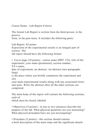
  • 21. I (A) V (V) I (A) (a) (b) Fig. 1. A sample current-voltage characteristic for an ohmic (a) and a non-ohmic (b) device. The resistance of a given ohmic conductor increases with length and decreases for larger cross-sectional area. For a conductor of uniform cross section A and length the resistance R can be computed as: R = ρ , (Eqn. 3) where the proportionality constant ρ is the electrical resistivity of the material measured in ohm-meters, Ωm. While the resistance of a device depends on its geometry, the resistivity is specific for the material used in the device and depends on the nature of the material and on temperature but not on its shape or size. The resistivity is the inverse of conductivity ρ = . For all metals resistivity increases with temperature. For conductors the resistivity changes approximately linearly with temperature over a limited range of temperature according to the following formula ρ = ρo [1 + α (T- T0)], (Eqn. 4) where ρ is the resistivity at temperature T (in ºC), ρo is the resistivity at some reference temperature T0 (usually 20º C), and α is called the temperature coefficient of resistivity expressed in . Since resistance is proportional to resistivity a similar expression is true for the resistance dependence on temperature: R = R0 [1 + α (T – T0)] (Eqn. 5)
  • 22. PROCEDURE Part 1. Determining the resistance of a pencil lead. The Ohm’s law can be used to find electrical properties, namely the resistance, of any conductor. In this part of the experiment you will apply the Ohm’s Law to determine the resistance of a virtual pencil lead. You will measure the current through the pencil lead and the voltage drop across this element for a few output voltages delivered by the battery. Next, you will present the data graphically, plotting I PENCIL vs. v PENCIL, and analyze the plot to find the resistance of the simulated pencil. Open the PhET Interactive Simulations web page http://phet.colorado.edu/en/simulation/circuit-construction-kit- dc-virtual-lab and download the Circuit Construction Kit (DC Only), Virtual Lab. Using the circuit components from the right tool menus and the Grab Bag options (that is where you find the pencil lead) construct the circuit similar to the one shown in Fig.2. Please, note that the ammeter is connected in series with the pencil while the voltmeter leads are attached to the pencil tips in parallel fashion (the red lead of the meter touches the pencil end of the higher potential and the black lead is connected to the end of the lower potential). , Fig. 2. Circuit for measuring the resistance of the pencil lead. Right click on the battery allows you to select the Voltage Change option which opens the voltage selection window as seen in Fig.2. For your convenience, please, leave this window open for easy access. By adding the internal resistance of the battery we will make this circuit behaving even more life-like – right click on the battery again and change its internal resistance to 9 Ω. Apply 5 different voltages from the battery, ranging from 0 to 100 Volts and evenly spread. After adjusting
  • 23. the battery voltage to the desired value, close the switch and record the current measured by the ammeter, I PENCIL , and the voltage detected by the voltmeter, V PENCIL. Open the LoggerPro program available in MyApps on My ASU site. The default screen contains a two-column data table and a graph window. Enter the V PENCIL data (expressed in Volts, V) in the first column, and the I PENCIL values (expressed in Amperes, A) in the second column. Double click the heading of each column to change its name (X → V, Y → I), enter the units for the typed-in data and select the number of decimal places you wish to be displayed. Create a new calculated column for the resistance R expressed in ohms, Ω. Hint: To add a calculated column to the data table select “Data” in the upper tool bar options, and then “New Calculated Column…”. In the equation field type “V”/”I”, where V and I should be chosen from the pull down Variables selection. After entering the experimental data in the table you should automatically see them being plotted in the graph window. As a good scientific habit you always want to show only the collected data points without the lines in-between them. So, double click on the graph window and uncheck the option “Connect Points”. Apply the linear fit to your set of data. Double click on the small window with the fit parameters and select show uncertainty. From the slope calculate the resistance of the virtual pencil. Propagate the uncertainty in the slope into the uncertainty of the experimental resistance of the pencil. Re- scale the whole graph window to about half of the available screen space, without covering the data table. Insert a second graph displaying the resistance calculated in the third column on both axis of the new graph. Again, uncheck the “Connect Points” option. Re-scale this graph window to fit into the space remaining on the page. By dragging around with the mouse, select all data points of this plot and apply statistics from the Analyze menu. Save the LoggerPro file for future reference. How does the mean value displayed in the statistics window compare to the resistance computed from the slope of the first
  • 24. graph? State the measured resistance of the virtual pencil lead along with its uncertainty. Remember to express the uncertainty with just one (or maximum two) sig figure(s) and adjust the number of decimal places in the main result appropriately. Based on your data conclude whether the virtual pencil was an ohmic element or not. Capture the screen with the LoggerPro file and paste it into MS Word – you will have to attach it to your lab report. It is recommended to use the landscape orientation for the page layout in MS Word. If you assume that the virtual pencil lead was made out of material of resistivity ρ = 3.510-4 Ωm (a composition of graphite) and the diameter of the lead was 0.6 mm, how long was the pencil? On average the real pencil rod has a diameter of 2.4 mm and the length of 18.0 cm. If it was made of the same material as the virtual pencil what resistance would it have? Propagate the errors in the dimension measurements into the final uncertainty of the calculated resistance. Part 2. Investigating the resistive properties of a light bulb. Using Firefox login to VirtualPhysicsLabs: http://virtuallabs.ket.org/physics/. Click the Labs tab and select lab 16 -DC Circuits. Before running the simulation read the full description and detailed information. Connect the circuit shown below. Make sure to keep the default setting for the wire resistance at 0 Ω. Please, note that the ammeter must always be connected in series with the investigated object (the light bulb in our case) to measure the current flowing through it, while the voltmeter is wired in parallel with the object to show the potential difference across it without disturbing the current distribution within the circuit. Click the battery and adjust its voltage to 1 V. Double click the switch to close the circuit. Open a new file in LoggerPro and
  • 25. record the first pair of data: the voltage across the light bulb as measured by the voltmeter and the current displayed by the ammeter. Remember to label the column headings appropriately and enter the units. Since the internal resistance of the ammeter is negligible, there is no potential drop across this instrument and the voltage across the light bulb equals the output voltage from the battery. Next, open the switch. Change the battery output signal to 2 V, close the switch and record the new values for the current and voltage of the light bulb. Open the switch and repeat the same procedure for the following voltages from the battery: 4 V, 6 V, 8 V, 10 V, 20 V, 30 V, 40 V, 50 V and 60 V. Add a new calculated column to the data table showing the resistance of the bulb, expressed in Ω, as determined from Ohm’s law. Now, assuming that the filament of the bulb is made of tungsten for which the temperature coefficient of resistivity is α = 4.5 10-3 1/°C, and the resistance of the bulb at T0= 20 °C is R0= 10 Ω, create yet another calculated column displaying the temperature of the bulb. Hint: Rearrange eqn. 5 to get a direct relationship of T = f(R). Insert a new graph showing the filament temperature T (Y-axis) vs. the filament resistance R(X-axis). Apply the linear fit to your set of data of T vs. R. Re-size both graph windows (I vs. V and T vs. R) so they nicely fit on one page along with the data table. Save your LogegrPro file for future reference. Based on the graph of I vs. V for the light bulb what can you conclude: is the bulb an ohmic or a non-ohmic circuit element? Finally, calculate the ratio rR of the resistance of the bulb at 60 V to its resistance at 1 V. Also, compute a similar ratio rT for the corresponding bulb temperatures. Which parameter: the filament resistance or its temperature was increasing with a faster rate? Capture the screen with the LoggerPro file and paste it into MS Word – you will have to attach it to your lab report. It is recommended to use the landscape orientation for the page layout in MS Word.
  • 26. * Include answers to all questions in lab report Page 6 of 6 Page 1 of 6 DC CIRCUITS I (Ohm’s Law) OBJECTIVES: • To apply Ohm’s Law to find the resistance of a virtual pencil lead. • To investigate the behavior of a light bulb in a simple DC circuit. EQUIPMENT: Computer with Internet access. INTRODUCTION AND THEORY: The main concepts in the analysis of DC (direct current = current of constant magnitude and direction) electric circuits are: Ohm’s Law and resistance, Kirchhoff’s loop rule (sometimes called the voltage law), Kirchhoff’s junction rule (also called the current law), and the power relationship.
  • 27. I. Ohm’s Law and Resistance. The Ohm’s Law describes an empirical relationship and it can be expressed on a microscopic level or on a macro scale. On the atomic level the law states that the ratio of the current density J (= current per unit area) to the electric field E is constant and independent of the electric field producing the current as follows: � � = σ = const (Eqn. 1) where J is the current density ( J ≡ � � = nqvd), E represents the electric field established in the material/conductor as a result of a potential difference applied and maintained across the conductor, and σ is the conductivity of the material. On a macro scale Ohm’s Law can be presented as �
  • 28. � = R = const (Eqn. 2) which is the same as I = � � , and it means the electric current I which flows through a conductor is directly proportional to the voltage V applied to it. The ratio R is called the electrical resistance and is being one of the most basic properties of any electrical device represents simply its ability to oppose the passage of an electric current resulting from the voltage applied to the device. Referring to the atomic Page 2 of 6 level the electrical resistance of an object arises from the random collisions between the free electrons carrying the current with fixed atoms of the material. This repeated process causes scattering of the electrons and makes them drift in the direction opposite that of the internal electric field. If V is in Volts and I is in Amperes, R is in ohms, Ω.
  • 29. Materials which have a constant resistance over a considerable range of applied voltages or currents for a given temperature are said to be ohmic. For such materials/devices the plot of I vs. V (usually called the “I-V characteristic”) is a straight line passing through the origin and the reciprocal of the slope represents the resistance of the device. Ohmic objects with a very low resistance and thus being able to transfer current with the least loss of electrical energy are called conductors. Example: electrical wires. Materials that have non-linear I-V curve, which resistance changes with voltage or current, are called non-ohmic. Example: semiconductor diodes, transistors. (a) (b) Fig. 1. A sample current-voltage characteristic for an ohmic (a) and a non-ohmic (b) device. The resistance of a given ohmic conductor increases with length and decreases for larger cross- sectional area. For a conductor of uniform cross section A and length � the resistance R can be
  • 30. computed as: R = ρ � , (Eqn. 3) where the proportionality constant ρ is the electrical resistivity of the material measured in ohm- meters, Ωm. While the resistance of a device depends on its geometry, the resistivity is specific for the material used in the device and depends on the nature of the material and on temperature but not on its shape or size. The resistivity is the inverse of conductivity ρ = � . For all metals V (V) R = � ��� = constant
  • 31. I (A) V (V) I (A) Page 3 of 6 resistivity increases with temperature. For conductors the resistivity changes approximately linearly with temperature over a limited range of temperature according to the following formula ρ = ρo [1 + α (T- T0)], (Eqn. 4) where ρ is the resistivity at temperature T (in ºC), ρo is the resistivity at some reference temperature T0 (usually 20º C), and α is called the temperature coefficient of resistivity expressed in °� . Since resistance is proportional to resistivity a similar expression is true for the resistance dependence on temperature:
  • 32. R = R0 [1 + α (T – T0)] (Eqn. 5) PROCEDURE Part 1. Determining the resistance of a pencil lead. The Ohm’s law can be used to find electrical properties, namely the resistance, of any conductor. In this part of the experiment you will apply the Ohm’s Law to determine the resistance of a virtual pencil lead. You will measure the current through the pencil lead and the voltage drop across this element for a few output voltages delivered by the battery. Next, you will present the data graphically, plotting I PENCIL vs. v PENCIL, and analyze the plot to find the resistance of the simulated pencil. Open the PhET Interactive Simulations web page http://phet.colorado.edu/en/simulation/circuit- construction-kit-dc-virtual-lab and download the Circuit Construction Kit (DC Only), Virtual Lab. Using the circuit components from the right tool menus and the Grab Bag options (that is where you find the pencil lead) construct the circuit similar to the one shown in Fig.2. Please, note that the ammeter is
  • 33. connected in series with the pencil while the voltmeter leads are attached to the pencil tips in parallel fashion (the red lead of the meter touches the pencil end of the higher potential and the black lead is connected to the end of the lower potential). Page 4 of 6 , Fig. 2. Circuit for measuring the resistance of the pencil lead. Right click on the battery allows you to select the Voltage Change option which opens the voltage selection window as seen in Fig.2. For your convenience, please, leave this window open for easy access. By adding the internal resistance of the battery we will make this circuit behaving even more life-like – right click on the battery again and change its internal resistance to 9 Ω. Apply 5 different voltages from the battery, ranging from 0 to 100 Volts and evenly spread. After adjusting the battery voltage to the desired value, close the switch and record the current measured by the ammeter, I PENCIL , and the
  • 34. voltage detected by the voltmeter, V PENCIL. Open the LoggerPro program available in MyApps on My ASU site. The default screen contains a two- column data table and a graph window. Enter the V PENCIL data (expressed in Volts, V) in the first column, and the I PENCIL values (expressed in Amperes, A) in the second column. Double click the heading of each column to change its name (X → V, Y → I), enter the units for the typed-in data and select the number of decimal places you wish to be displayed. Create a new calculated column for the resistance R expressed in ohms, Ω. Hint: To add a calculated column to the data table select “Data” in the upper tool bar options, and then “New Calculated Column…”. In the equation field type “V”/”I”, where V and I should be chosen from the pull down Variables selection. After entering the experimental data in the table you should automatically see them being plotted in the graph window. As a good scientific habit you always want to show only the collected data points without the lines in-between them. So, double click on the graph window and uncheck the option “Connect
  • 35. Points”. Apply the linear fit to your set of data. Double click on the small window with the fit parameters and select show uncertainty. From the slope calculate the resistance of the virtual pencil. Propagate the uncertainty in the slope into the uncertainty of the experimental resistance of the pencil. Page 5 of 6 Re-scale the whole graph window to about half of the available screen space, without covering the data table. Insert a second graph displaying the resistance calculated in the third column on both axis of the new graph. Again, uncheck the “Connect Points” option. Re- scale this graph window to fit into the space remaining on the page. By dragging around with the mouse, select all data points of this plot and apply statistics from the Analyze menu. Save the LoggerPro file for future reference. How does the mean value displayed in the statistics window compare to the resistance computed from the slope of the first graph? State the measured resistance of the virtual pencil lead along with its uncertainty. Remember to
  • 36. express the uncertainty with just one (or maximum two) sig figure(s) and adjust the number of decimal places in the main result appropriately. Based on your data conclude whether the virtual pencil was an ohmic element or not. Capture the screen with the LoggerPro file and paste it into MS Word – you will have to attach it to your lab report. It is recommended to use the landscape orientation for the page layout in MS Word. If you assume that the virtual pencil lead was made out of material of resistivity ρ = 3.5×10⁻⁴ Ωm (a composition of graphite) and the diameter of the lead was 0.6 mm, how long was the pencil? On average the real pencil rod has a diameter of 2.4 ± 0.1 mm and the length of 18.0 ± 0.1 cm. If it was made of the same material as the virtual pencil what resistance would it have? Propagate the errors in the dimension measurements into the final uncertainty of the calculated resistance. Part 2. Investigating the resistive properties of a light bulb. Using Firefox login to VirtualPhysicsLabs: http://virtuallabs.ket.org/physics/. Click the Labs tab and select
  • 37. lab 16 -DC Circuits. Before running the simulation read the full description and detailed information. Connect the circuit shown below. Make sure to keep the default setting for the wire resistance at 0 Ω. Please, note that the ammeter must always be connected in series with the investigated object (the light bulb in our case) to measure the current flowing through it, while the voltmeter is wired in parallel with Page 6 of 6 the object to show the potential difference across it without disturbing the current distribution within the circuit. Click the battery and adjust its voltage to 1 V. Double click the switch to close the circuit. Open a new file in LoggerPro and record the first pair of data: the voltage across the light bulb as measured by the voltmeter and the current displayed by the ammeter. Remember to label the column headings appropriately and enter the units. Since the internal resistance of the ammeter is negligible, there is no potential drop across this instrument and the voltage across the
  • 38. light bulb equals the output voltage from the battery. Next, open the switch. Change the battery output signal to 2 V, close the switch and record the new values for the current and voltage of the light bulb. Open the switch and repeat the same procedure for the following voltages from the battery: 4 V, 6 V, 8 V, 10 V, 20 V, 30 V, 40 V, 50 V and 60 V. Add a new calculated column to the data table showing the resistance of the bulb, expressed in Ω, as determined from Ohm’s law. Now, assuming that the filament of the bulb is made of tungsten for which the temperature coefficient of resistivity is α = 4.5× 10⁻³ 1/°C, and the resistance of the bulb at T0= 20 °C is R0= 10 Ω, create yet another calculated column displaying the temperature of the bulb. Hint: Rearrange eqn. 5 to get a direct relationship of T = f(R). Insert a new graph showing the filament temperature T (Y-axis) vs. the filament resistance R(X-axis). Apply the linear fit to your set of data of T vs. R. Re-size both graph windows (I vs. V and T vs. R) so they nicely fit on one page along with the data table. Save your LogegrPro file for future reference. Based on the graph of I vs. V for the light bulb what can you conclude: is the bulb an ohmic or a non-
  • 39. ohmic circuit element? Finally, calculate the ratio rR of the resistance of the bulb at 60 V to its resistance at 1 V. Also, compute a similar ratio rT for the corresponding bulb temperatures. Which parameter: the filament resistance or its temperature was increasing with a faster rate? Capture the screen with the LoggerPro file and paste it into MS Word – you will have to attach it to your lab report. It is recommended to use the landscape orientation for the page layout in MS Word. * Include answers to all questions in lab report Current and Resistance Electric Current Electric current is the rate of flow of charge through some region of space. The SI unit of current is the ampere (A). 1 A = 1 C / s The symbol for electric current is I. Section 27.1
  • 40. Average Electric Current Charges are moving perpendicular to a surface of area A. ΔQ is the amount of charge that passes through A in time Δt. The average current: Section 27.1 Instantaneous Electric Current If the rate at which the charge flows varies with time, the instantaneous current, I, is defined as the differential limit of average current as Δt→0. Section 27.1 Direction of Current It is conventional to assign to the current the same direction as the flow of positive charges. In an ordinary conductor, the direction of current flow is opposite the direction of the flow of electrons. It is common to refer to any moving charge as a charge carrier. Section 27.1 Charge Carrier Motion in a Conductor
  • 41. The zigzag black lines represents the motion of a charge carrier in a conductor in the presence of an electric field. The net motion of electrons is opposite the direction of the electric field. Section 27.1 Current & Drift Speed The total charge is: ΔQ = (nAΔx)q The current is Iave = ΔQ/Δt = nqvdA vd = = Δx/Δt is an average speed called the drift speed. Section 27.1 Current Density Current density is defined as the current per unit area. J ≡ I / A = nqvd J has SI units of A/m2 The current density is in the same direction as the flow of positive charges. Section 27.2 Conductivity For some materials, the current density is directly proportional to the electric field. The constant of proportionality, σ, is called the conductivity of the conductor. Section 27.2
  • 42. Ohm’s Law Ohm’s law states that for many materials, the ratio of the current density to the electric field is a constant σ that is independent of the electric field producing the current. J = σ E Section 27.2 Ohm’s Law Materials that obey Ohm’s law are said to be ohmic. However, Not all materials follow Ohm’s law. Materials that do not obey Ohm’s law are said to be nonohmic. Section 27.2 Resistance In a conductor, the voltage drop across the ends of the conductor is proportional to the current through the conductor. The constant of proportionality is called the resistance of the conductor. SI units of resistance are ohms (Ω). 1 Ω = 1 V / A Section 27.2 Resistors Most electric circuits use circuit elements called resistors to control the current in the various parts of the circuit. Values of resistors are normally indicated by colored bands. Section 27.2
  • 43. Resistivity The inverse of the conductivity is the resistivity: ρ = 1 / σ Resistivity has SI units of ohm-meters (Ω . m) Resistance is also related to resistivity: Section 27.2 Resistance & Resistivity Every ohmic material has a characteristic resistivity that depends on the properties of the material and on temperature. Resistivity is a property of substances. The resistance of a material depends on its geometry and its resistivity. Resistance is a property of an object. Section 27.2 Ohmic and Nonohmic An ohmic devices (a) The slope is related to the resistance. Section 27.2 Nonohmic devices are those whose resistance changes with voltage or current (b). Resistivity & Temperature The resistivity of a conductor varies approximately linearly
  • 44. with the temperature. ρo is the resistivity at some reference temperature To (usually taken to be 20°C) α is the temperature coefficient of resistivity The temperature coefficient of resistivity can be expressed as: Temperature Variation of Resistance Since the resistance of a conductor is proportional to the resistivity, you can find the effect of temperature on resistance. R = Ro[1 + α(T - To)] Section 27.4 Electric Power The power is given by the equation P = I ΔV Alternative expressions can be found: Units: I is in A, R is in Ω, ΔV is in V, and P is in W