Decision Theory LEARNING OBJECTIVES SUPPLEMENT OUTLINE 5S.5 Decision Making under Uncertainty, 219 After completing this supplement, you 5S.6 Decision Making under Risk, 220 5S.1 Introduction, 216 should be able to: 5S.7 Decision Trees, 2215S.2 The Decision Process and Causes of L05S.1 Outline the steps in the decision Poor Decisions, 217 5S.8 Expected Value of Perfect process. Information, 2235S.3 Decision Environments, 218 L05S.2 Name some causes of poor 5S.9 Sensitivity Analysis, 224 decisions. 5S.4 Decision Making under Certainty, 218 L05S.3 Describe and use techniques that apply to decision making under uncertainty. L05S.4 Describe and use the expected- value approach. L05S.5 Construct a decision tree and use it to analyze a problem. L05S.6 Compute the expected value of perfect information. L05S.7 Conduct sensitivity analysis on a simple decision problem. 55.1 INTRODUCTION - Decision theory represents a general approach to decision making. It is suitable for a wide range of operations management decisions. Among them are capacity planning, product and service design, equipment selection, and location planning. Decisions that lend themselves to a decision theory approach tend to be characterized by the following elements: 1. A set of possible future conditions that will have a bearing on the results of the decision. 2. A list of alternatives for the manager to choose from. 3. A known payoff for each alternative under each possible future condition. To use this approach, a decision maker would employ this process: 1. Identify the possible future conditions (e.g., demand will be low, medium, or high; the competitor will or will not introduce a new product). These are called states of nature. 2. Develop a list of possible alternatives, one of which may be to do nothing. t 3. Determine or estimate the payoff associated with each alternative for every possible future condition. ---- ----------------------------------------~-- 216 217 Supplement to Chapter Five Decision Theory If possible, estimate the likelihood of each possible future condition. 5. Evaluate alternatives according to some decision criterion (e.g., maximize expected profit), and select the best alternative. The information for a decision is often summarized in a payoff table, which shows the expected payoffs for each alternative under the various possible states of nature. These tables are helpful in choosing among alternatives because they facilitate comparison of alternatives. Consider the following payoff table, which illustrates a capacity planning problem. POSSIBLE FUTURE DEMAND Alternatives Low Moderate High Small facility $10* $10 $10 Medium facility 7 12 12 Large facil ity (4) 2 16 'Present value in $ millions. The payoffs are shown in the body of the table. In this instance, the payoffs are in terms of present values, which represent equivalent current dollar values of expected future income.

1. Decision Theory
LEARNING OBJECTIVES SUPPLEMENT OUTLINE 5S.5
Decision Making under Uncertainty, 219
After completing this supplement, you 5S.6 Decision Making
under Risk, 220 5S.1 Introduction, 216
should be able to: 5S.7 Decision Trees, 2215S.2 The Decision
Process and Causes of
L05S.1 Outline the steps in the decision Poor Decisions, 217
5S.8 Expected Value of Perfect
process. Information, 2235S.3 Decision Environments, 218
L05S.2 Name some causes of poor 5S.9 Sensitivity Analysis,
224
decisions. 5S.4 Decision Making under Certainty, 218
L05S.3 Describe and use techniques that
apply to decision making under
uncertainty.
L05S.4 Describe and use the expected-
value approach.
L05S.5 Construct a decision tree and use
it to analyze a problem.
L05S.6 Compute the expected value of
perfect information.
L05S.7 Conduct sensitivity analysis on a
simple decision problem.

2. 55.1 INTRODUCTION
-
Decision theory represents a general approach to decision
making. It is suitable for a wide
range of operations management decisions. Among them are
capacity planning, product and
service design, equipment selection, and location planning.
Decisions that lend themselves to
a decision theory approach tend to be characterized by the
following elements:
1. A set of possible future conditions that will have a bearing on
the results of the decision.
2. A list of alternatives for the manager to choose from.
3. A known payoff for each alternative under each possible
future condition.
To use this approach, a decision maker would employ this
process:
1. Identify the possible future conditions (e.g., demand will be
low, medium, or high; the
competitor will or will not introduce a new product). These are
called states of nature.
2. Develop a list of possible alternatives, one of which may be
to do nothing.
t
3. Determine or estimate the payoff associated with each
alternative for every possible
future condition.

3. ---- ----------------------------------------~--
216
217 Supplement to Chapter Five Decision Theory
If possible, estimate the likelihood of each possible future
condition.
5. Evaluate alternatives according to some decision criterion
(e.g., maximize expected
profit), and select the best alternative.
The information for a decision is often summarized in a payoff
table, which shows the
expected payoffs for each alternative under the various possible
states of nature. These tables
are helpful in choosing among alternatives because they
facilitate comparison of alternatives.
Consider the following payoff table, which illustrates a capacity
planning problem.
POSSIBLE FUTURE DEMAND
Alternatives Low Moderate High
Small facility $10* $10 $10
Medium facility 7 12 12
Large facil ity (4) 2 16
'Present value in $ millions.

4. The payoffs are shown in the body of the table. In this instance,
the payoffs are in terms
of present values, which represent equivalent current dollar
values of expected future income
less costs. This is a convenient measure because it places all
alternatives on a comparable
basis. If a small facility is built, the payoff will be the same for
all three possible states of
nature. For a medium facility, low demand will have a present
value of $7 million, whereas
both moderate and high demand will have present values of $12
million. A large facility will
have a loss of $4 million if demand is low, a present value of $2
million if demand is moder-
ate, and a present value of $16 million if demand is high.
The problem for the decision maker is to select one of the
alternatives, taking the present
value into account.
Evaluation of the alternatives differs according to the degree of
certainty associated with
the possible future conditions.
5S.2 THE DECISION PROCESS AND CAUSES
OF POOR DECISIONS
Despite the best efforts of a manager, a decision occasionally
turns out poorly due to unfore-
seeable circumstances. Luckily, such occurrences are not
common. Often, failures can be
traced to a combination of mistakes in the decision process, to
bounded rationality, or to
suboptimization.

5. The decision process consists of these steps:
1. Identify the problem.
2. Specify objectives and criteria for a solution.
3. Develop suitable alternatives.
4. Analyze and compare alternatives.
5. Select the best alternative.
6. Implement the solution.
7. Monitor to see that desired result is achieved.
In many cases, managers fail to appreciate the importance of
each step in the decision-
making process. They may skip a step or not devote enough
effort to completing it before
jumping to the next step. Sometimes this happens owing to a
manager's style of making quick
decisions or a failure to recognize the consequences of a poor
decision. The manager's ego can
be a factor. This sometimes happens when the manager has
experienced a series of successes-
important decisions that turned out right. Some managers then
get the impression that they can
do no wrong. But they soon run into trouble, which is usually
enough to bring them back down
Payoff table Table showing
the expected payoffs for each
alternative in every possible state
of nature.

6. L05S.1 Outline the steps in
the decision process.
L05S.2 Name some causes of
poor decisions.
••
218
Bounded rationality The
limitations on decision making
caused by costs, human abilities,
time, technology, and availability
of information.
Suboptimization The result
of different departments each
attempting to reach a solu-
tion that is optimum for that
department.
Certainty Environment in
which relevant parameters have
known values.
Risk Environment in which cer-
tain future events have probable
outcomes.
Uncertainty Environment in
which it is impossible to assess
the likelihood of various future

7. events.
EXAMPLE
55-1
Supplement to Chapter Five Decision Theory
to earth. Other managers seem oblivious to negative results and
continue the process they
associate with their previous successes, not recognizing that
some of that success may have
been due more to luck than to any special abilities of their own.
A part of the problem may be
the manager's unwillingness. to admit a mistake. Yet other
managers demonstrate an inability
to make a decision; they stall long past the time when the
decision should have been rendered .
Of course, not all managers fall into these traps-it seems safe to
say that the majority
do not. Even so, this does not necessarily mean that every
decision works out as expected.
Another factor with which managers must contend is bounded
rationality, or the limits
imposed on decision making by costs, human abilities, time,
technology, and the availability
of information. Because of these limitations, managers cannot
always expect to reach deci-
sions that are optimal in the sense of providing the best possible
outcome (e.g., highest profit,
least cost). Instead, they must often resort to achieving a
satisfactory solution.
Still another cause of poor decisions is that organizations
typically departmentalize deci-
sions. Naturally, there is a great deal of justification for the use

8. of departments in terms of
overcoming span-of-control problems and human limitations.
However, suboptimization can
occur. This is a result of different departments' attempts to
reach a solution that is optimum
for each. Unfortunately, what is optimal for one department may
not be optimal for the orga-
nization as a whole. If you are familiar with the theory of
constraints (see Chapter 16), subop-
timization and local optima are conceptually the same, with the
same negative consequences.
5S.3 DECISION ENVIRONMENTS
Operations management decision environments are classified
according to the degree of cer-
tainty present. There are three basic categories: certainty, risk,
and uncertainty.
. Certainty means that relevant parameters such as costs,
capacity, and demand have
known values.
Risk means that certain parameters have probabilistic outcomes.
Uncertainty means that it is impossible to assess the likelihood
of various possible future
events.
Consider these situations:
1. Profit per unit is $5. You have an order for 200 units. How
much profit will you make?
(This is an example of certainty since unit profits and total
demand are known.)
2. Profit is $5 per unit. Based on previous experience, there is a

9. 50 percent chance of an
order for 100 units and a 50 percent chance of an order for 200
units. What is expected
profit? (This is an example of risk since demand outcomes are
probabilistic.)
3. Profit is $5 per unit. The probabilities of potential demands
are unknown. (This is an
example of uncertainty.)
The importance of these different decision environments is that
they require different anal-
ysis techniques. Some techniques are better suited for one
category than for others.
5S.4 DECISION MAKING UNDER CERTAINTY
When it is known for certain which of the possible future
conditions will actually happen, the
decision is usually relatively straightforward: Simply choose the
alternative that has the best
payoff under that state of nature. Example 5S-1 illustrates this.
Determine the best alternative in the payoff table on the
previous page for each of-the cases: It
is known with certainty that demand will be (a) low, (b)
moderate, (c) high.
219
'------~
Supplement to Chapter Five Decision Theory
Choose the alternative with the highest payoff. Thus, if we

10. know demand will be low, we
would elect to build the small facility and realize a payoff of :
10 million. If we know demand
will be moderate, a medium factory would yield the highest
payoff ($12 million versus either
$10 million or $2 million). For high demand, a large facility
would provide the highest payoff.
Although complete certainty is rare in such situations, this kind
of exercise provides some
perspective on the analysis. Moreover, in some instances, there
may be an opportunity to con-
sider allocation of funds to research efforts, which may reduce
or remove some of the uncer-
tainty surrounding the states of nature, converting uncertainty
to risk or to certainty.
5S.5 DECISION MAKING UNDER UNCERTAINTY
At the opposite extreme is complete uncertainty: 0 information
is available on how likely
the various states of nature are. Under those conditions, four
possible decision criteria
are maximin, maximax, Laplace, and minimax regret. These
approaches can be defined as
follows:
Maximin-Determine the worst possible payoff for each
alternative, and choose the
alternative that has the "best worst." The maximin approach is
essentially a pessimistic
one because it takes into account only the worst possible
outcome for each alternative.
The actual outcome may not be as bad as that, but this approach
establishes a "guaranteed
minimum."

11. Maximax-Determine the best possible payoff, and choose the
alternative with that pay-
off. The maximax approach is an optimistic, "go for it" strategy;
it does not take into
account any payoff other than the best.
Laplace-Determine the average payoff for each alternative, and
choose the alternative
with the best average. The Laplace approach treats the states of
nature as equally likely.
Minimax regret-Determine the worst regret for each alternative,
and choose the alter-
native with the "best worst." This approach seeks to minimize
the difference between the
payoff that is realized and the best payoff for each state of
nature.
The next two examples illustrate these decision criteria.
Referring to the payoff table on page 217, determine which
alternative would be chosen under
each of these strategies:
a. Maximin
b. Maximax
c. Laplace
a. Using maximin, the worst payoffs for the alternatives are as
follows:
Small facility: $10 million
Medium facility: 7 million

12. Large facility: -4 million
Hence, since $10 million is the best, choose to build the small
facility using the maximin
strategy.
b. Using maximax, the best payoffs are as follows:
Small facility: $10 million
Medium facility: 12 million
Large facility: 16 million
The best overall payoff is the $16 million in the third row.
Hence, the maximax criterion
leads to building a large facility.
SOLUTION
L05S.3 Describe and use
techniques that apply to deci-
sion making under uncertainty.
Maximin Choose the alterna-
tive with the best of the worst
possible payoffs.
Maximax Choose the alter-
native with the best possible
payoff.
Laplace Choose the alternative
with the best average payoff of
any of the alternatives.
Minimax regret Choose the

13. alternative that has the least of
the worst regrets.
EXAMPLE
5S-2
eXcel
mhhe.com/stevenson12e
SOLUTION
220
I #
EXAMPLE
5S-3
SOLUTION
Regret (opportunity loss)
The differencebetween a given
payoff and the best payoff for a
state of nature.
L05S.4 Describe and use the
expected-value approach.
Expected monetary value
(EMV) criterion The best
expected value among the
alternatives.
Supplement to Chapter Five Decision Theory

14. c. For the Laplace criterion, first find the row totals, and then
divide each of those amounts
by the number of states of nature (three in this case). Thus, we
have
Row Total
(in $ millions)
Row Average
(in $ millions)
Small facility
Medium facility
Large facility
$30
31
14
$10.00
10.33
4.67
Because the medium facility has the highest average, it would
be chosen under the Laplace
criterion.
Determine which alternative would be chosen using a minimax
regret approach to the capac-
ity planning program.
The first step in this approach is to prepare a table of regrets (or
opportunity losses). To do

15. this, subtract every payoff in each column from the best payoff
in that column. For instance,
in the first column, the best payoff is 10, so each of the three
numbers in that column must be
subtracted from 10. Going down the column, the regrets will be
10 - 10 = 0, 10 - 7 = 3, and
10 - (-4) = 14. In the second column, the best payoff is 12.
Subtracting each payoff from
12 yields 2, 0, and 10. In the third column, 16 is the best
payoff. The regrets are 6, 4, and 0.
These results are summarized in a regret table:
REGRETS (IN $ MILLIONS)
Alternatives Low Moderate High Worst
,Small facility $0 $2 $6 $6
Medium facility 3 0 4 4
Large facility 14 10 0 14
The second step is to identify the worst regret for each
alternative. For the first alternative,
the worst is 6; for the second, the worst is 4; and for the third,
the worst is 14.
The best of these worst regrets would be chosen using minimax
regret. The lowest regret is
4, which is for a medium facility. Hence, that alternative would
be chosen.
Solved Problem 6 at the end of this supplement illustrates
decision making under uncer-
tainty when the payoffs represent costs.
The main weakness of these approaches (except for Laplace) is
that they do not take into

16. account all of the payoffs. Instead, they focus on the worst or
best, and so they lose some
information. Still, for a given set of circumstances, each has
certain merits that can be helpful
to a decision maker.
5S.6 DECISION MAKING UNDER RISK
Between the two extremes of certainty and uncertainty lies the
case of risk: The probability
of occurrence for each state of nature is known. (Note that
because the states are mutually
exclusive and collectively exhaustive, these probabilities must
add to 1.00.) A widely used
approach under such circumstances is the expected monetary
value criterion. The expected
value is computed for each alternative, and the one with the best
expected value is selected.
The expected value is the sum of the payoffs for an alternative
where each payoff is weighted
by the probability for the relevant state of nature. Thus, the
approach is
Expected monetary value (EMV) criterion-Determine the
expected 'payoff or each
alternative, and choose the alternative that has the best expected
payoff.
Supplement to Chapter Five Decision Theory
Using the expected monetary value criterion, identify the best
alternative for the previous
payoff table for these probabilities: low = .30, moderate = .50,
and high = .20.

17. Find the expected value of each alternative by multiplying the
probability of occurrence for
each state of nature by the payoff for that state of nature and
summing them:
= .30($10)
= .30($7)
= .30($-4)
EVsmall
EVmedium
EVlarge
.50($10)
.50($12)
.50($2)
+ .20($10) = $10
.20($12) = $10.5
.20($16) = $3
+
+
+
+
+
Hence, choose the medium facility because it has the highest
expected value.
The expected monetary value approach is most appropriate

18. when a decision maker is nei-
ther risk averse nor risk seeking, but is risk neutral. Typically,
well-established organizations
with numerous decisions of this nature tend to use expected
value because it provides an indi-
cation of the long-run, average payoff. That is, the expected-
value amount (e.g., $10.5 million
in the last example) is not an actual payoff but an expected or
average amount that would be
approximated if a large number of identical decisions were to be
made. Hence, if a decision
maker applies this criterion to a large number of similar
decisions, the expected payoff for the
total will approximate the sum of the individual expected
payoffs.
55.7 DECISION TREES
In health care the array of treatment options and medical costs
makes tools such as decision
trees particularly valuable in diagnosing and prescribing
treatment plans. For example, if a
20-year-old and a 50-year-old both are brought into an
emergency room complaining of chest
pains, the attending physician, after asking each some questions
on family history, patient his-
tory, general health, and recent events and activities, will use a
decision tree to sort through
the options to arrive at the appropriate decision for each patient.
Decision trees are tools that have many practical applications,
not only in health care but
also in legal cases and a wide array of management decision
making, including credit card
fraud; loan, credit, and insurance risk analysis; decisions on
new product or service develop-
ment; and location analysis.

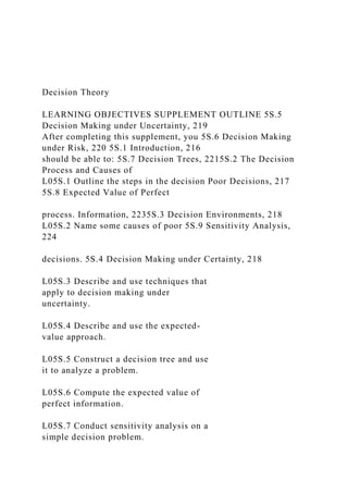
19. A decision tree is a schematic representation of the alternatives
available to a decision
maker and their possible consequences. The term gets its name
from the treelike appearance
of the diagram (see Figure 5S.1). Although tree diagrams can be
used in place of a payoff
Payoff 1
Payoff 2
>-,
~e
°CJ",o
Payoff 3
Initial
decision
Payoff 4
C-?
00
6'(9
~ Payoff 5
Payoff 6
• Decision point o Chance event
221
EXAMPLE
55-4

20. mhhe.com/stevenson12e
l05S.5 Construct a decision
tree and use it to analyze a
problem.
Decision tree A schematic
representation of the available
alternatives and their possible
consequences.
FIGURE 5S.1
Format of a decision tree
eXcel
mhhe.com/stevenson12e
222
EXAMPLE
55-5
SOLUTION
Supplement to Chapter Five Decision Theory
table, they are particularly useful for analyzing situations that
involve sequential decisions.
For instance, a manager may initially decide to build a small
facility only to discover that
demand is much higher than anticipated. In this case, the
manager may then be called upon to
make a subsequent decision on whether to expand or build an
additional facility.

21. A decision tree is composed of a number of nodes that have
branches emanating from them
(see Figure 5S.1). Square nodes denote decision points, and
circular nodes denote chance
events. Read the tree from left to right. Branches leaving square
nodes represent alternatives;
branches leaving circular nodes represent chance events (i.e.,
the possible states of nature).
After the tree has been drawn, it is analyzed from right to left;
that is, starting with the
last decision that might be made. For each decision, choose the
alternative that will yield the
greatest return (or the lowest cost). If chance events follow a
decision, choose the alternative
that has the highest expected monetary value (or lowest
expected cost).
A manager must decide on the size of a video arcade to
construct. The manager has narrowed
the choices to two: large or small. Information has been
collected on payoffs, and a decision
tree has been constructed. Analyze the decision tree and
determine which initial alternative
(build small or build large) should be chosen in order to
maximize expected monetary value.
o ./;' $40
{'O~
N'l
0e
..0

22. ,,~~ $40
~0'V.
)0
Overtime $50
E:'JrIJ
Cillo
$55
,,~~ ($10)
~0'V.
)0
o ./;'
{'O~
Reo.
N'l
0e..0 liCe
IJric $50es
High
oerr,
Cillo $70(.6)
S,..
"110-:ge
The dollar amounts at the branch ends indicate the estimated
payoffs if the sequence of
chance events and decisions that is traced back to the initial
decision occurs. For example, if
the initial decision is to build a small facility and it turns out

23. that demand is low, the payoff
will be $40 (thousand). Similarly, if a small facility is built,
demand turns out high, and a later
decision is made to expand, the payoff will be $55 (thousand).
The figures in parentheses on
branches leaving the chance nodes indicate the probabilities of
those states of nature. Hence,
the probability of low demand is .4, and the probability of high
demand is .6. Payoffs in
parentheses indicate losses.
Analyze the decisions from right to left:
1. Determine which alternative would be selected for each
possible second decision. For a
small facility with high demand, there are three choices: do
nothing, work overtime, and
expand. Because expand has the highest payoff, you would
choose it. Indicate this by
placing a double slash through each of the other alternatives.
Similarly, for a large facility
with low demand, there are two choices: do nothing and reduce
prices'Xcsa would choose
reduce prices because it has the higher expected value, so a
double slash is placed on the
other branch.
Supplement to Chapter Five Decision Theory 223
Determine the product of the chance probabilities and their
respective payoffs for the
remaining branches:
Build small

24. Low demand .4($40) = $16
High demand .6($55) = $33
Build large
Low demand .4($50) = 20
High demand .6($70) = $42
Determine the expected value of each initial alternative:
Build small $16 + $33 = $49
Build large $20 + $42 = .62
Hence, the choice should be to build the large facility because it
has a larger expected
value than the small facility .
.8 EXPECTED VALUE OF PERFECT
INFORMATION
certain situations, it is possible to ascertain which state of
nature will actually occur in the
e. For instance, the choice of location for a restaurant may
weigh heavily on whether a
- . highway will be constructed or whether a zoning permit will
be issued. A decision maker
have probabilities for these states of nature; however, it may be
possible to delay a deci-
until it is clear which state of nature will occur. This might
involve taking an option to
_.; the land. If the state of nature is favorable, the option can be
exercised; if it is unfavorable,
option can be allowed to expire. The question to consider is

25. whether the cost of the option
ill be less than the expected gain due to delaying the decision
(i.e., the expected payoff
ve the expected value). The expected gain is the expected value
of perfect information,
EVPI.
Other possible ways of obtaining perfect information depend
somewhat on the nature of
- decision being made. Information about consumer preferences
might come from market
ch, additional information about a product could come from
product testing, or legal
rts might be called on.
There are two ways to determine the EVPL One is to compute
the expected payoff under
enainty and subtract the expected payoff under risk. That is,
Expected value of Expected payoff Expected payoff (5S-1)
perfect information under certainty under risk
"':-singthe information from Example 5S-4, determine the
expected value of perfect informa-
n using Formula 5S-1.
-=- t, compute the expected payoff under certainty. To do this,
identify the best payoff under
h state of nature. Then combine these by weighting each payoff
by the probability of that
e of nature and adding the amounts. Thus, the best payoff under
low demand is $10, the
t under moderate demand is 12, and the best under high demand

26. is $16. The expected
yoff under certainty is, then,
.30($10) + .50($12) + .20($16) = $12.2
L05S.6 Compute the expected
value of perfect information.
Expected value of perfect
information (EVPI) The
difference between the expected
payoff with perfect information
and the expected payoff
under risk.
EXAMPLE
5S-6
SOLUTION #
224
I~
EXAMPLE
5S-7
eXcel
mhhe.com/stevenson12e
SOLUTION
Ul5S.7 Conduct sensitivity

27. analysis on a simple decision
problem.
Sensitivity analysis Deter-
mining the range of probability
for which an alternative has the
best expected payoff.
EXAMPLE
5S-8
eXcel
mhhe.com/stevenson12e
SOLUTION
Supplement to Chapter Five Decision Theory
The expected payoff under risk, as computed in Example 5S--4,
is $10.5. The EVPI is the dif-
ference between these:
EVPI = $12.2 - $10.5 = $1.7
This figure indicates the upper limit on the amount the decision
maker should be willing
to spend to obtain perfect information in this case. Thus, if the
cost equals or exceeds this
amount, the decision maker would be better off not spending
additional money and simply
going with the alternative that has the highest expected payoff.
A second approach is to use the regret table to compute the
EVPI. To do this, find the
expected regret for each alternative. The minimum expected
regret is equal to the EVPI.

28. Determine the expected value of perfect information for the
capacity-planning problem using
the expected regret approach.
Using information from Examples 5S-2, 5S-3, and 5S--4, we can
compute the expected regret
for each alternative. Thus: '
Small facility
Medium facility
Large facility
+ .20(6) = 2.2
+ .20(4) = 1.7 [minimum]
+ .20(0) = 9.2
.30(0)
.30(3)
.30(14)
+ .50(2)
+ .50(0)
+ .50(10)
The lowest expected regret is l.7, which is associated with the
second alternative. Hence, the
EVPI is $l.7 million, which agrees with the previous example
using the other approach.
5S.9 SENSITIVITY ANALYSIS
Generally speaking, both the payoffs and the probabilities in
this kind of a decision problem
are estimated values. Consequently, it can be useful for the

29. decision maker to have some
indication of how sensitive the choice of an alternative is to
changes in one or more of these
values. Unfortunately, it is impossible to consider all possible
combinations of every variable
in a typical problem. Nevertheless, there are certain things a
decision maker can do to judge
the sensitivity of probability estimates.
Sensitivity analysis provides a range of probability over which
the choice of alternatives
would remain the same. The approach illustrated here is useful
when there are two states of
nature. It involves constructing a graph and then using algebra
to determine a range of prob-
abilities for which a given solution is best. In effect, the graph
provides a visual indication
of the range of probability over which the various alternatives
are optimal, and the algebra
provides exact values of the endpoints of the ranges. Example
5S-8 illustrates the procedure .•.•.
Given the following table, determine the range of probability
for state of nature #2, that is,
P(2), for which each alternative is optimal under the expected-
value approach.
STATE OF
NATURE
#1 #2
A 4 12
Alternative B 16 2
C 12 8

30. First, plot each alternative relative to P(2). To do this, plot the
#1 value on the left side of the
graph and the #2 value on the right side. For instance, for
alternative A, plot 4 on the left side
of the graph and 12 on the right side. Then connect these two
points with a straight line. The
three alternatives are plotted on the graph as shown on the next
page.
Supplement to Chapter Five Decision Theory 225
16 16
14
12
10
#2
8 Payoff
6
4
2
.8 1.0
14
12

31. 10
#1
Payoff 8
6 I
I
4 I
I
2 I
--B best--~C best-i~--
o .2 .4 .6
P(2)
The graph shows the range of values of P(2) over which each
alternative is optimal. Thus,
low values of P(2) [and thus high values of P(l), since P(l) +
P(2) = 1.0], alternative B
have the highest expected value; for intermediate values of
P(2), alternative C is best; and
higher values of P(2), alternative A is best.
To find exact values of the ranges, determine where the upper
parts of the lines intersect.
e that at the intersections, the two alternatives represented by
the lines would be equivalent
terms of expected value. Hence, the decision maker would be
indifferent between the two
:nat point. To determine the intersections, you must obtain the
equation of each line. This
relatively simple to do. Because these are straight lines, they
have the form y = a + bx,

32. - e a is the y-intercept value at the left axis, b is the slope of the
line, and x is P(2). Slope
fined as the change in y for a one-unit change in x. In this type
of problem, the distance
'een the two vertical axes is 1.0. Consequently, the slope of
each line is equal to the right-
value minus the left-hand value. The slopes and equations are as
follows:
#1 #2 Slope Equation
4 12 12 - 4 = + 8 4 + 81'1:2)
16 2 2 -16 = -14 16 - 141'1:2)
12 8 8-12=- 4 12-41'1:2)
From the graph, we can see that alternative B is best from P(2)
5 0 to the point where that
ight line intersects the straight line of alternative C, and that
begins the region where C is
r. To find that point, solve for the value of P(2) at their
intersection. This requires setting
two equations equal to each other and solving for P(2). Thus,
16 - 14P(2) = 12 - 4P(2)
Rearranging terms yields
4 = lOP(2)
olving yields P(2) = AO. Thus, alternative B is best from P(2) =
0 up to P(2) = AO. B
C are equivalent at P(2) = AO.
Alternative C is best from that point until its line intersects

33. alternative A's line. To find that
ection, set those two equations equal and solve for P(2). Thus,
+ 8P(2) = 12 - 4P(2)
Rearranging terms results in
12P(2) = 8
olving yields P(2) = .67. Thus, alternative C is best from P(2) >
AO up to P(2) = .67,
re A and C are equivalent. For values of P(2) greater than .67 up
to P(2) = 1.0, A is best.
. ote: If a problem calls for ranges with respect to P(l), find the
P(2) ranges as above, and
subtract each P(2) from 1.00 (e.g., AO becomes .60, and .67
becomes .33).
226
SUMMARY
.. "
KEY TERMS
SOLVED PROBLEMS
Problem 1
eXcel
mhhe.com/stevenson12e

34. Solution
Problem 2
eXcel
mhhe.com/stevenson12e