Psyc 355 Effective Communication / snaptutorial.com
bayes_proj
1. • July 2016 •
Bayesian Linear vs Ordered
Probit/Logit Models for ordinal data:
fitting student scores in two
Portuguese High schools
Tommaso Guerrini∗
Politecnico di Milano
tommaso.guerrini@mail.polimi.it
Abstract
Assessing which factors influence student scores has long been scope of work among social
scientists. Scores are a typical example of ordinal discrete data, but is general wisdom to treat them as
continuous once the number of levels is over 6. In this paper I went into linear and ordered regression
models, assessing performance both in fitting/prediction and computational expense terms.
I. Introduction
A
ssessing which factors influence stu-
dent scores has long been scope of
work among social scientists. Scores
are a typical example of ordinal discrete data,
but is general wisdom to treat them as continu-
ous once the number of levels is over 6. In this
paper I went into linear and ordered regres-
sion models, assessing performance both in
fitting/prediction and computational expense
terms. Literature is wide on whether a given
predictor has a positive, null or negative influ-
ence over a student result in a test. The interest
lays on different levels. First and foremost re-
searchers try to assess which family, habitat
and leisure time patterns are favorable in order
to help the student achieve good marks. Many
papers have been written regarding the rela-
tionship between parents’ education or parents’
job and their child performance. Furthermore,
the fact that the social environment in which
children are raised deeply influences their aca-
demic and even professional career has become
common knowledge in this reasearch field. A
second important topic researchers have tried
to address regards the teaching performance
in different educational institutions, often as a
government enquiry in trying to establish the
best program to follow and award good teach-
ers and good schools. In the dataset considered
a wide number of covariates spans through
these two topics. Nevertheless, if interpret-
ing the results can be catchy, the biggest deal
of attention has been given to the statistical
instruments to perform such analysis. As is
typical in Social Sciences data are often cat-
egorical both in the response (suggesting to
explore less known regression methods) and
in the covariates. Purpose of the author was
to compare different methods, always from
a Bayesian perspective, even when prior in-
formations are pretty fragmentary. All the
models used are presented together with sam-
pling methods and references to the code used.
An Appendix gives further information about
data exploration, MCMC diagnostics, posterior
∗Master Degree in Applied Statistics
1
2. • July 2016 •
plots and full prediction results.
II. The Dataset and Preliminary
Work
Data are student scores in two different schools
in Portugal. Along with the scores of first and
second semester there is a set of 30 covariates.
The number of statistical units is 631. The data
were gathered in 2008 and can be found on the
well-known UCI repository (see reference).
name type levels
school binary 0, 1
sex binary 0, 1
age numerical 15to22
famsize binary 0, 1
Pstatus binary 0, 1
Medu categorical 1, 2, 3, 4
Fedu categorical 1, 2, 3, 4
Mjob categorical 1, 2, 3, 4, 5
Fjob categorical 1, 2, 3, 4, 5
reason categorical 1, 2, 3
guardianm binary 0, 1
traveltime ordinal 1to4
studytime ordinal 1to4
failures numerical 1to4
schoolsup binary 0, 1
famsup binary 0, 1
paid binary 0, 1
activities binary 0, 1
nursery binary 0, 1
higher binary 0, 1
internet binary 0, 1
romantic binary 0, 1
famrel ordinal 1to5
freetime ordinal 1to5
goout ordinal 1to5
Dalc ordinal 1to5
Walc ordinal 1to5
health ordinal 1to5
absences numerical 0to93
Table 1: Dataset description, see references for levels
meaning
A total of 423 student scores were
gathered in school 1 (GP), 208 in school 0
(MS). One of the first modification to the
data was to the categorical data. For in-
stance, a variable like Mother Education
(Medu) has 5 different levels, corresponding to
’teacher’,’health’,’home’,’services’ and ’other’.
Numerical labels 1 to 5 have no mathemati-
cal meaning since working in civil services (4)
it’s not equivalent to four times working as a
teacher(1). So variables of this type were trans-
formed in k-1 dummies, where k equals the
number of levels.
unit Medu
1 teacher
2 home
3 services
4 health
5 other
unit teacherm health services home
1 1 0 0 0
2 0 0 0 1
3 0 0 1 0
4 0 1 0 0
5 0 0 0 0
Table 2: Transforming categorical variables
with k levels into k-1 dummies.
This way a student with mother job
in ’other’ category is still represented since it
corresponds to a 0 into the other 4 categories.
That guarantees linear independence in the de-
sign matrix once the regression was performed
and results not reported here confirm the bet-
ter fitting of the model to the data once the
variable transformation was made, both in R2
and other diagnostics. Student scores had a 0-
20 scale, but 0,1 were excluded since they were
probably linked to a missing value. This was
not specified once the data were gathered. Yet,
data excluded were a dozen and this did not
influence the model built. In the final dataset
there were present just marks from 4 to 19
with frequencies specified in the next table. A
very low presence of values 4,5,6,18,19 reduces
2
3. • July 2016 •
the significant levels to 11, which approaches
the literature number of 6 for which linearity
assumption of the response is not correct.
First of all a division of the dataset
in a training and a test set was made: 480 ob-
servations in the training set and 151 in the
test set. Naturally the partition was not made
randomly, instead units were selected in both
set so that the frequencies of the response lev-
els were proportional to the whole set. For
instance, if a mark 6 had a relative frequency
of 8% of the whole dataset, so was in the train-
ing and test part. This point is pretty crucial
in the ordered models, since the number of
tresholds equals the number of response levels
- 1, making their training of uttermost impor-
tance. The main reason for this division was to
assess differences among models in prediction
terms. Another frequency to take into account
when dividing the dataset was that of the two
schools: since there were 423 observations for
school GP and 208 for school MS I maintained
a 2:1 ratio in both training and test set. Instead,
I chose to set regression coefficients on the first
semester grades G1, so frequencies of G2 (2nd
semester grade) were not considered.
I. A BoxCox transformation
Classical linear regression models, assume nor-
mality of the response given a set of covariates.
The normal distribution support is , i.e. a con-
tinuous support who takes also negative values.
Furthermore the normal distribution is sym-
metric with a maximum centered in the mean
as high as the variance is low. When mod-
eling linear responses we look for these fea-
tures and when not present there’s a variety of
’tricks’ one can use before quitting and looking
somewhere else. In the work considered two
characteristics of the response do not respect
the assumptions: the response is strictly pos-
itive and it is ordinal. Ordinality was treated
deeply given that generalized linear models
which account for it were used and later pre-
sented fully. As regards the positive support
literature is wide: usually transformations like
log Y or
√
Y are suggested when dealing with
a positive response Y. The best way to find
the best transformation of the response such
that requirements of a linear model are met is
the boxcox transformation (with one parame-
ter if the transformation required is a canonical
one as the ones mentioned above): Yλ
i =
Yλ
i −1
λ
if λ = 0, Yλ
i = ln λ if λ = 0. This is auto-
matically implemented through the R software.
Even if a 0.4 value maximizes the like-
lihood, I still chose 0.5 being a known trans-
formation (
√
Y) less computational expensive.
Even with this transformation, which improved
the R2, diagnostics remained not particularly
satisfactory giving further motivations to build
a non linear model.
III. Bayesian Linear Models
In frequentist statistics a regression model con-
sists of a response Y whose expected value
E[Y] depends linearly on a set of covarites X,
through coefficients β . We say that: Yi =
Xi ∗ β + i , i ∼ N(0, σ2), while β are the OLS
estimates (deterministic) and sigma is fixed
too. In a bayesian context, the parameters of
the model are not fixed, but random, so we
must give a prior distribution to β and σ2 and
then know how to compute the posterior of
these parameters, so that we can make infer-
ence. Posterior ∝ Likelihood ∗ Prior , so that
the choice of the prior directly affects the Pos-
terior distribution. Yet, in our case, we have
a peculiar set of covariates such that no prior
information can be used in set mean and vari-
3
4. • July 2016 •
ance of our parameters. An idea would be
to divide the training set in 2 parts, finding
the ols estimates of β and set them as b0 and
then compute the likelihood and the posterior
on the second part of the training set. Un-
fortunately this procedure gave estimates just
slightly different from the ones obtained with
noninformative priors and no prediction power
improvement. Furthermore, reducing the num-
ber of data with a model with so many param-
eters (41) could make our model not so good.
We need a prior specification for our param-
eters π(β, σ2) . First of all, there’s an inter-
esting property for such a prior writing it like:
π(β, σ2) = π(β|σ2) * π(σ2) . In this case, choos-
ing a Normal distribution for π(β|σ2) and an
Inverse-Gamma distribution for π(σ2) we have
a conjugate model to the normal Likelihood
specified at the beginning of the paragraph.
This really simplifies our calculations because
the posterior distribution will still be a prod-
uct of a Normal for an Inverse-Gamma, with
updated parameters.
β|σ2 ∼ N(b0, σ2 ∗ B0) (1)
σ2 ∼ Inv − Gamma(ν0
2 ,
(ν0∗σ2
0 )
2 ) (2)
Y|X, β, σ2 ∼ Nn(X ∗ β, σ2 ∗ I) (3)
π(β, σ2|Y) = π(β|σ2, Y)*π(σ2|Y) (4)
β|σ2, Y, X ∼ (bn, σ2 ∗ Bn) (5)
σ2|Y, X ∼ Inv − Gamma(νn
2 ,
νn∗σ2
n
2 ) (6)
.
This was the model used when the
training set was divided in 2 parts, with b0 =
βols and a Diagonal Matrix with σ2
βi
for B0 .
σ2 in that case was known and equal to the σ2
ols,
i.e. the residual standard error squared.
Another option used was the Zell-
ner’s g prior:
β|σ2, X ∼ Np(b0, B0) with B0 =
c ∗ (X ∗ X)−1
σ2 ∼ Inv − Gamma(0
2 ,
0∗σ2
0
2 ) ∝ 1
σ2 ∗
1(0, +∞)(σ2)
Of course we need X’X invertible. The
Zellner’s prior is conjugate to the normal likeli-
hood. Different values of c where tried giving
more or less weight to the prior specificaton.
As before also the Zellner’s g prior was used
when setting previous ols estimates as mean of
the β.
The last option considered is a ref-
erence prior i.e. Jeffreys prior based on
Fisher information, in particular π(β, σ2) ∝
det(I(β, σ2)), where I(β, σ2) is the Fisher
information Matrix. This is just π(β, σ2) ∝
1
σ2 ∗ 1(0, +∞)(σ2) .
I. LPML and choice of prior
To choose between the 3 different priors elic-
itated above it was used the LPML i.e. the
LogPosteriorMarginalLikelihood. LPML =
∑ log(CPOi) where CPOi = L(Yi|Y−i) is the
Conditional Predictive Ordinate i.e. the predic-
tive distribution of unit Yi given all the other
units in the training set minus i. The model
with the highest LPML was always chosen and
in particular the noninformative Jeffreys prior
seemed to fit the data in the training set the
best. In the codes an uninformative prior was
obtained by setting a high variance over both
the Regression coefficients β and the error vari-
ance σ2.
4
5. • July 2016 •
IV. ordered models
Generalized linear models appear when the
response variable in a regression model is not
linear. Briefly: the ingredients in a GLM are
a random component (Y), a sistematic compo-
nent ηi , which is la linear combination of our
covariates, such that ηi = Xi ∗ β and a link func-
tion g(), which relates E[Yi] and ηi, such that
g(E[Yi]) = ηi. It is the choice of this function
which generates the 2 models implemented
in this work, the ordered logit model and the
ordered probit one.
I. GLM for binary responses
Let’s consider the case in which the response
is binary:
Yi|Xi ∼ Be(π) .
In this case E[Yi] = 1 ∗ P(Yi = 1)+ =
+P(Yi = 0) = π
so I want to specify a function g(π) = ηi =
Xi ∗ β .
Let’s consider the inverse link func-
tion g()−1 = F(), πi = F(Xi ∗ β), and let’s
finally define:
1. a logit model, where F(t) =
1
1+exp(−t)
;
2. a probit model, where F(t) =
Φ(t) =
t
−∞ φ(z)dz, where φ is the standard
normal density and Φ is the CDF.
II. cumulative links
We want to consider the ordering of our re-
sponse variable, so let’s define cumulative
probabilities as P(Y ≤ j|X) = π1(X) + ... +
πj(X), j = 1, ..., J, where J is the number of lev-
els of the response and πj(X) is the probability
of the binary outcome Yi = j . What is desired
now is to link the cumulative probabilities to
the linear predictor ηi = Xi ∗ β . Based on
the function we choose, as in the binary case,
different links:
1. logit(P(Y ≤ j|X)) = β0j
+ β−0 ∗ X−0
2. probit(P(Y ≤ j|X)) = β0j
+ β−0 ∗ X−0
j = 1, ..., J − 1 .
First, let’s consider the fact that the
intercept (β0j
) varies for any level j, while the
other coefficients (β−0) are the same for any
level: this is known as a Proportional − odds
model.
III. latent variables
Now let’s consider an interpretation of the
model which also makes the computation more
interpretable. Let’s introduce the presence of
a latent variable and show calculations just for
the probit model (for the logit ones we just
need to substitute the normality assumption
for the error term with a logistic density):
Y∗
i = Xi ∗ β + i, epsiloni ∼ N(0, σ2
) (1)
What we want to do now is to stabi-
lize a correspondence between the latent vari-
able Y∗
i and the observed ordinal one Yi , to do
that we need tresholds:
Yi = 0 ⇐⇒ Y∗
i ≤ τ1
Yi = j ⇐⇒ τj < Y∗
i ≤ τj+1 j = 1, ..., J − 1
Yi = J ⇐⇒ Y∗
i > τj .
Of course our J-1 tresholds obey: τ1 < ... < τJ .
5
6. • July 2016 •
Now we plug in the cumulative link
mentioned before:
P(Yi = 0) = P(Y∗
i ≤ tau1) = P( i ≤
τ1 − Xi ∗ β) = Φ(τ1−Xi∗β
σ )
P(Yi = j) = Φ(
τj+1−Xi∗β
σ ) − Φ(
τj−Xi∗β
σ )
j = 1, ..., J − 1
P(Yi = J) = 1 − Φ(τ1−Xi∗β
σ ) .
Given n observations the likelihood for this
model is:
L = ∏n
1 ∏
J
0(Φij − Φi,j−1)Z
ij
where Φij = Φ[(τj − X ∗ β)/σ], and Zij = 1 if
Yi = j 0 otherwise.
IV. Bayesian Ordered Probit(Logit)
Model
β , τ and σ are not jointly identified, for
instance consider shifting the treshold
parameters, such that we should shift also the
intercept in β, but what if then we also change
the scale σ ? The ordered probit model is
typically identified with sets of normalizing
constraints for the 3 sets of parameters. The
ones used in the codes, giving same inferential
results are in the next table.
β σ τ
unconstrained fixed=1 one fixed, τ1 = 0
drop intercept fixed=1 unconstrained
Now let’s build up the bayesian model. As
said before we assume regression coefficients
and thresholds independent a priori:
π(β, τ) = π(β) ∗ π(τ) .
β ∼ N(b0, B0)
Priors for τ have just to respect the ordering of
the constraints, the one we used was the prior
considered by Albert and Chib (1993), which
proposed an improper-yet-coherent prior for τ,
uniform over the polytope T ⊂ J:
T =
tau = (τ1, ..., τj−1) ∈ j : τj > τj−1, ∀j = 2, ..., J
. This improper prior is easily implemented in
JAGS as shown after.
V. sampling
First of all we must say that if sampling
methods can become rather complex, for
instance in the specification of full
conditionals in a Gibbs Sampler, the software
at our disposal makes things easier. While R
presents lots of built in function for Bayesian
Regression, both linear and non linear, JAGS
automatically calculates the full conditionals.
In the code section I’ll present both the R and
JAGS code. If we consider a conjugate model
(as all the ones considered before), sampling is
straightforward. In fact we can generate a
MonteCarlo sample in the following way:
Sample β(t) from (1)
β|σ2, Y, X ∼ (bn, σ2 ∗ Bn) (1)
Sample σ2 from (2)
σ2|Y, X ∼ Inv − Gamma(νn
2 ,
νn∗σ2
n
2 ) (2)
This is the most general case, with parameters
meaning already specified above. As seen in
the Bayesian Linear Models section posterior
distributions parameters become simpler in
the case of a g or a reference/uninformative
prior.
The sampling is not trivial in the Ordered
Models case. There is no conjugate prior that
can be exploited and τ parameters make the
sampling more difficult. The strategy adopted
was that of the Albert and Chib (1993)
data-augmented Gibbs Sampler, I’ll report the
procedure as in Jackman:
1. sample Y∗
i , i = 1, ..., n given β, σ2, τ, Yi and
Xi from a truncated normal density
Y∗
i |Xi, β, σ2, τ, Yi = j ∼
N(Xiβ, σ2) ∗ 1τYi
< Y∗
i ≤ τYi+1
where I introduce τ0 = −∞ for Yi = 0
(or lowest level) and τJ+1 for Yi = J.
2. sample β given the latent Y∗ and X from a
Normal density, with mean
b = (B−1
0 + X X)(B−1
0 b0 + X Y∗) and variance
6
7. • July 2016 •
B = (B−1
0 + X X)−1. All parameters are then
specified in the Code section, but just to
mention it here I’ll set b0 = 0 and B0 = 104 to
make them as uninformative as possible (R
does it automatically, but results are the same
with JAGS);
3. sample τ from their conditional densities,
given the latent data Y∗ . There are 2 ways to
implement this:
3.1 (Albert and Chib) , for τj sample uniformly
from the interval
[max(max(Y∗
i |Yi =
j − 1), τj−1)], min(min(Y∗
i |Yi = j), τj+1)]
3.2 (Cowles(1996)) proposed a Metropolis
scheme for sampling all the vector of
thresholds τ en bloc. This makes it much
quicker, even if, as shown in the diagnostics,
has a high autocorrelation in the samples of τ,
imposing a higher thinning then 3.1
VI. Simple and Hierarchical
Models
The purpose of a linear model is to find a
relation between the student score and the
covariates as universal as possible. The ideal
model would be able to fit new scores from
the same ’environment’ (i.e. student scores in
2009, considering no major changes in the 2
schools regarding teaching and scores policy),
without being computationally expensive (by
reducing the number of predictors). The
models considered are:
model data fixed eff. random eff.
1 trainingGP XGP none
2 trainingMS XMS none
3 training X none
4 training X school
5 training X X
Data is the set used to perform regression, GP
and MS indicate data relatively just to school
GP or MS.
Models 1 through 3 are as the ones specified
in the ’Bayesian linear Models’ section, with a
Jeffreys prior. We expect the first 2 models to
fit very well data in the school they refer to,
but we don’t know if they’ll fit as well data in
the other school (they would if there’s no big
difference between the two). The third model
is a first attempt to reach a synthesis between
the two schools and it should be a good one in
case the two dataset are sort of generated from
the same underlying population. In the
prediction section crosspopulation predictions
will not be reported, i.e. we won’t use MS
school coefficients to perform prediction on
TestGP, or viceversa. A first question could be:
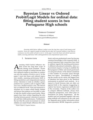
why do we build a 4th and a 5th model? An
answer for the Xschool mixed-effect is shown in
the next figure which represents the boxplots
of the student scores in the 2 schools in the
training set. We can see a positive offset in
school GP, while the underlying distribution is
pretty much the same.
In that case the model is (with Yi =
√
G1):
E[Yi] = Xi ∗ β + Xschooli
∗ γschooli
γschooli
∼ N(0, σ2
s )
Here γschool is the mixed effect parameter
associated to the covariate Xschool which is
equal to 1 for school GP. Note that we could
have not introduced this covariate, by adding
a mixed effect on the intercept since they both
act by shifting the intercept. Prior specification
for β and σ2 are the same as before, and we
used a noninformative prior given the LPML
results. As for σ2
s , I just introduce the school
covariate in the design matrix X and still used
7
8. • July 2016 •
a noninformative prior. Instead in the JAGS
code I implemented I put σ2
s ∼ U(0, 10), a 0
mean for β, a 106 diagonal for Σ (covariance
matrix of the regression coefficients) and
another Inv − Gamma(0.001, 0.001) for σ2.
What about model number 5? Let’s say I don’t
need it, what would I expect? First of all I
know I’ve already fitted model 1 and 2 and I
could look at the distribution of the
parameters there: if I spot major differences in
mean/mode of the distributions of some
covariates, then I know I’ll need a mixed effect
on those. Let’s see that effect for a couple of
covariates like sex and schoolsup, showing the
sample from the posterior distributions of βsex
in the probit model and βschoolsup in the linear
one, from model 1(Blue) and 2(Red).
Coefficients are small because we are dealing
with the square root of the score, yet we can
see a difference in the due graphs: while
female perform better in GP there’s pretty
much no effect in school MS; a greater
difference, which seems very important in
dividing the 2 schools is found in the
schoolsupport, positive effect in MS and even
a negative one in GP. I’ll show the results for
schoolsup also for the ordered probit model,
which are the same for all covariates not
considering a rescaling factor.
In the end the model is:
E[Yi] = Xi ∗ β + Xi ∗ γschooli
γschooli
∼ Np(0, Σγ)
Σγ ∼ Inv − Wishart(r, rR)
As regards the prior parameters for the
covariance matrix of the mixed effects I set
them as uninformative as possible, with r
equalling p (number of regressors) and R
being a diagonal matrix with 0.1 entries.
However JAGS does not have an
Inverse-Wishart sampler so I set the covariance
matrix of the mixed effect as the correlation
matrix of the predictors in it (from the training
set). Naturally in JAGS I put the inverse of
this matrix since distributions are in terms of
precisions. An important note regarding the
full mixed effects models: I estimated
parameters both for the LM and GLM after
performing variable selection. This was due to
computation reasons: JAGS required a lifetime
to converge while the MCMCpack failed to.
I’ll next show the results of the sampling, in
particular I’ll concentrate on the mixed effects
8
9. • July 2016 •
distributions and compare them to the fixed
effects.
Model 4 for Ordered Probit Regression
ηi = Xiβ + γschooli
P(Yi = j) = Φ(
τj+1−ηi
σ ) − Φ(
τj−ηi
σ )
Yi ∼ Dcat(p[i,])
Model 5 for Ordered Probit Regression
ηi = Xiβ + Xiγschooli
P(Yi = j) = Φ(
τj+1−ηi
σ ) − Φ(
τj−ηi
σ )
Yi ∼ Dcat(p[i,])
Next I show some of the posterior
distributions of fixed and random effects of
the hierarchical model, both for the probit and
the linear one.
An important note:
Because of incredibly slow-mixing I used a
strong approximation in some of the
computations for the Hierarchical ordered
probit, setting γGP = −γMS to speed up
convergence. In some cases I set
β0 =
βOLSGP
+βOLSMS
2 , γMS0
=
βOLSMS
−βOLSGP
2 .
That is shown in some of the plots in which
the mixed effects are symmetric.
In every plot I reported the posterior sample
of βpGP
and βpMS
, basically the coefficient p of
the simple models 1 and 2. Then I reported
the βp of the Hierarchical model, together
with γpGP
and γpMS
VII. variable selection
With such a high number of regressors
computations get much more expensive and
models less synthetic: it is then wise to adopt
a variable selection strategy.
In this work I used a Normal-Mixture of
Inverse-Gammas (NMIG), which both helps
selecting the proper model among the 2p
present (one for each subset of regressors) and
9
10. • July 2016 •
estimating the β. So I selected those regressors
whose 90% posterior credible interval did not
contain 0. I then verified these estimates
through a stepWise method based on Akaike
Information Criterion. I did not implement a
Variable Selection for the Hierarchical Models,
since computations were long especially for
the ordered probit model and models too
complex. I chose a different strategy: I kept all
the regressors which were significant for
model 1,2,3 (i.e. for school GP, school MS and
for the general one).
The model for variable selection is:
βi ∼ N(0, λk)
λk|v0, v1, γk, a, b ∼
(1 − γk) ∗ IG(a, v0
b ) + γk ∗ IG(a, v1
b )
γk|ωk ∼ Be(ωk)
ωk ∼ U(0, 1)
It’s a classical spike and slab priors model: we
induce positive probability on the hypothesis
H0 : βk = 0 .
Originally this was done by using a mixture of
Dirac measures concentrated in 0 (spike) and a
uniform diffuse component (slab). We see that
it is a hierarchical model where βk stands at
the lowest level and then the spike and slab
prior is over its variance λk . In the Jags code I
chose:
βk , k = 1, .., p
βk|γk ∼ N(0, 1−γk
τ2
+ γk
τ1
)
τ1 ∼ Gamma(a, b1)
τ2 ∼ Gamma(a, b2)
γk|wk ∼ Bernoulli(wk)
wk ∼ U(0, 1)
Results of variable selection for models 1
through 4 are shown in the next table.
name 1 2 3 4
intercept YES YES YES YES
school YES
sex YES YES YES
age
famsize
Pstatus YES
primarym
hsm
gradm YES YES YES
hsf
gradf
homem YES YES
servicesm
teacherm
healthm
homef YES
servicesf YES YES YES
teacherf YES YES YES
healthf
course
reputation YES YES
guardianm YES YES YES
guardianf
traveltime
studytime YES YES YES
failures YES YES YES YES
schoolsup YES YES YES
famsup
paid
activities
nursery
higher YES YES YES YES
internet
romantic
famrel YES
freetime
goout
Dalc
Walc YES
health YES
absences YES YES YES YES
Table 2: Variable Selection for models 1 through 4
10
11. • July 2016 •
VIII. Variable Selection for
Hierarchical Models
Since a variable selection method for a
Hierarchical model could be computationally
expensive, especially in the ordered probit
case, and moreover theoretically complex, I
decided to use a sort of empirical method,
mantaining in the design matrix X of the
Hierarchical Model both the covariates
selected in model 1 MS , model 2 GP and
model 3, but being considering 95% credible
intervals not containing 0.0. I chose to be more
restrictive since I found problems of
convergence both with the MCMChregress
and JAGS.
name YES/NO(90%) YES/NO(95%)
sex YES YES
age NO NO
famsize NO NO
Pstatus YES NO
primarym NO NO
hsm NO YES
gradm YES NO
hsf NO NO
gradf NO NO
homem YES NO
servicesm NO NO
teacherm NO NO
healthm NO NO
homef YES NO
servicesf YES NO
teacherf YES YES
healthf NO NO
course YES YES
reputation YES YES
guardianm YES NO
guardianf NO NO
traveltime NO NO
studytime YES YES
failures YES YES
schoolsup YES YES
famsup NO NO
paid NO NO
activities NO NO
nursery NO NO
higher YES YES
internet NO NO
romantic NO NO
famrel YES NO
freetime NO NO
goout NO NO
Dalc NO NO
Walc YES NO
health YES YES
absences YES YES
Table 3: Variable Selection for Hierarchical Models.
11
12. • July 2016 •
IX. results
To compare the different models that are used
it is considered the percentage of right guess
of student scores. From the theoretical
perspective basically mean of posterior
distribution of β were taken and it was
computed Y
p
new = E[Ynew] = Xβ to estimate
Ynew. Since this does not take into account the
variance I considered a right guess whenever
|Y
p
new − Ynew| < 0.5 in the continuous case,
while for ordinal data there was no need for
that of course. In Ordered models I used two
estimates for τ: the mean and the mode of the
posterior distribution. The mode gave better
results since, even after many samples, there
was no symmetric distribution (let’s not forget
the prior was a uniform one). Then I
computed Ynew = ∑K
i=1(P(Ynew = i) ∗ i) in one
case, Ynew = argmaxP(Ynew = j) in the other
and I reported the results for the second case.
I did not report the results for ordered logit
regression.
Model Linear/Probit Correct/Total %
1 Linear 23/151 15.2
2 Linear 25/151 16.6
3 Linear 21/151 13.9
4 Linear 21/151 13.9
1 Probit 35/151 23.2
2 Probit 52/151 34.4
3 Probit 48/151 31.8
4 Probit 52/151 34.4
Table 4: Results with a 0.5 error for Linear and Probit
Results are nothing spectacular, but we
already see a great improvement obtained
with the Probit Regression (using mean also
for τ). Let’s consider results with a 1.5 error
for the linear model (corresponding to a + − 1
in the score) and a 1.0 error in the probit one.
Model Linear/Probit Correct/Total %
1 Linear 64/151 42.4
2 Linear 73/151 48.3
3 Linear 73/151 48.3
4 Linear 74/151 49.0
1 Probit 81/151 53.6
2 Probit 92/151 60.9
3 Probit 96/151 63.6
4 Probit 92/151 60.9
Table 5: Results with a 1.5 error for Linear and 1.0 error
for Probit
Do results make sense? First of all we see that
GP model outperforms MS one and this
seems reasonable since there’s a 2:1 ratio
GP:MS in students from the 2 schools. Instead
there’s no significant improvement with model
3 and 4: if model 3 is a sort of average of the
models from the 2 different schools, model 4 is
too simple to fit more the data.
Let’s see the results after variable selection:
here we hope to lose no predictive power
while reducing the complexity of the model.
Model Linear/Probit Correct/Total %
1 Linear 23/151 15.2
2 Linear 25/151 16.6
3 Linear 25/151 16.6
4 Linear 29/151 19.2
1 Probit 45/151 29.8
2 Probit 52/151 34.4
3 Probit 50/151 33.1
4 Probit 56/151 37.1
Table 6: Results with a 0.5 error for Linear and no error
for Probit
As we hoped we don’t worse the results by
reducing the number of covariates. We also
see a little improvement in model 4: my
interpretation is that by reducing the noise
from the removed covariates we increase the
importance of the shift mixed effect.
12
13. • July 2016 •
X. JAGS and R code
1)JAGS code for simple Linear regression
(note how it requires the precision in place of
the variance)
model {
# Likelihood
for ( i in 1:N) {
mu[ i ] <− inprod ( x [ i , ] , beta [ ] )
y [ i ] ~ dnorm(mu[ i ] , tau )
}
# Prior for beta
for ( j in 1: p1 ) {
beta [ j ] ~ dnorm(0 ,1 e−08)
}
# Prior for the inverse variance
sigma ~ dunif (0 ,1 e−08)
tau <− pow( sigma , −2)
}
2)JAGS code for linear hierarchical model,
where scuola is school. Notice that JAGS is
not able to sample from a Wishart Distribution,
so I suggest you sample from it in R and then
you give it as a parameter in data list. Actually
I used the correlation matrix over the mixed
effects as variance and covariance matrix of the
multivariate normal distribution they are from.
model {
# Likelihood
for ( i in 1:N) {
mu[ i ] <− inprod ( x [ i , ] , beta [ ] ) +
inprod ( x [ i , ] , eta [ , scuola [ i ]+1])
y [ i ] ~ dnorm(mu[ i ] , tau )
}
# Prior for beta
for ( j in 1: p1 ) {
beta [ j ] ~ dnorm(0 ,1 e−08)
}
# Prior for eta ( mixed e f f e c t s )
for ( k in 1 : 2 ) {
eta [ k ] ~ dmnorm(0 ,B) #which equals :
# eta [ k ] ~ dmnorm
(0 , inverse ( dwish ( r ∗R, r ) ) )
}
# Prior for the inverse variance
sigma ~ dunif (0 ,1 e−08)
tau <− pow( sigma , −2)
}
3)Code for the simple Ordered Probit
regression.
model {
for ( i in 1:N) {
mu[ i ] <− inprod ( x [ i , ] , beta )
Q[ i , 1 ] <− phi ( tau [1]−mu[ i ] )
p[ i , 1 ] <− Q[ i , 1 ]
for ( j in 2 : 1 4 ) {
Q[ i , j ] <− phi ( tau [ j ]−mu[ i ] )
p[ i , j ] <− Q[ i , j ] − Q[ i , j −1]
}
p[ i , 1 5 ] <− 1 − Q[ i , 1 4 ]
y [ i ] ~ dcat (p[ i , 1 : 1 5 ] ) ## p[ i , ] sums to 1
}
beta [ 1 : p1 ] ~ dmnorm( b0 , B0 )
for ( j in 1 : 1 4 ) {
tau0 [ j ] ~ dnorm ( 0 , . 0 1 )
}
tau [ 1 : 1 4 ] <− sort ( tau0 )
}
4)Code for the Hierarchical Ordered Probit
regression.
5)Code for the Simple Ordered Logit
regression. To make code easier I shifted all
the scores to scores − 3 making them start
from 1.
model {
for ( i in 1:N) {
mu[ i ] <− inprod [ x [ i , ] , beta ]
l o g i t (Q[ i , 1 ] ) <− tau [1]−mu[ i ]
p[ i , 1 ] <− Q[ i , 1 ]
for ( j in 2 : 1 4 ) {
l o g i t (Q[ i , j ] ) <− tau [ j ]−mu[ i ]
p[ i , j ] <− Q[ i , j ] − Q[ i , j −1]
}
13
14. • July 2016 •
p[ i , 1 5 ] <− 1 − Q[ i , 1 4 ]
y [ i ] ~ dcat (p[ i , 1 : 1 5 ] )
}
## priors over betas
beta [ 1 : p1 ] ~ dmnorm( b0 [ ] , B0 [ , ] )
## thresholds
for ( j in 1 : 1 4 ) {
tau0 [ j ] ~ dnorm(0 , . 0 1 )
}
tau [ 1 : 1 4 ] <− sort ( tau0 )
}
6)Code for NMIG variable selection for
Linear Model (I won’t include the code for
Ordered Probit since it’s pretty much the
same)
model {
for ( i in 1:N) {
mu[ i ] <− inprod ( x [ i , ] , beta [ ] )
y [ i ] ~ dnorm(mu[ i ] , vart )
}
for ( j in 1: p1 )
{
gamma[ j ] ~ dbern (w[ j ] ) ;
beta [ j ] ~ dnorm(0 ,
pow(gamma[ j ]/ tau1 [ j ]+
(1−gamma[ j ])/ tau2 [ j ] , −1) ) ;
tau1 [ j ] ~ dgamma( 2 , 1 ) ;
tau2 [ j ] ~ dgamma( 2 , 1 0 0 0 ) ;
w[ j ] ~ dunif ( 0 , 1 ) ;
}
vart ~ dgamma( 0 . 0 0 1 , 0 . 0 0 1 )
}
Rcode
Code for Bayesian Linear Regression:
samples <− blinreg (Y, X,200000 , prior )
Where Y are the fitted values, X the design
matrix (include the intercept), 200000 number
of iterations, and prior the specification for the
Zellner’s prior, while the default one is the
uninformative. This function samples from the
joint posterior distribution (while JAGS
samples from the conditionals).
2.Code for the Ordered Probit Regression
mcmcprobitgp <− MCMCoprobit(G1 ~ XGP, data=traingp
burnin =1000 ,
mcmc=200000 ,
thin =50)
Here there are 2 ways of sampling: Cowles,
which is a Metropolis sampler and samples
the τ enbloc or AC (Albert and Chib (2001)).
3. Code for the Bayesian Hierarchical
regression
h i e r l s <− MCMChregress( fixed =
sqrt (G1) ~ X, random = ~ X,
group=" school " , data=train ,
burnin =100000 ,mcmc=200000 ,
thin =100 ,
r=q ,R=diag ( rep ( 0 . 0 1 , r ) ) )
XI. a Bivariate model?
A possible way to improve the model would
be to consider jointly G1 and G2, grades of the
first and second semester and see if the
additional information given by the 1st
semester vote improves the prediction power
while not increasing too much the
computational complexity.
Another idea is that the extreme levels of the
response variable, like 4,5,18,19 could be
omitted in the ordered probit model, since
they strongly harden the model, by
introducing additional thresholds parameters.
14
15. • July 2016 •
XII. MCMCconvergence
I will not show all the traceplots, autocorrelation and posterior samples plots.
1) Posterior samples and autocorrelation plots from linear model 2, of school GP.
15
27. • July 2016 •
6) A comparison in terms of computational expense between the Linear and Probit model.
Model Linear/Probit Iterazioni Thinning
GP Linear 104 10
MS Linear 104 10
βschool Linear 104 10
Mix Linear 2 ∗ 105 200
GP Probit 2 ∗ 105 200
MS Probit 2 ∗ 105 200
βschool Probit 2 ∗ 105 200
Mix Probit 5 ∗ 106 5 ∗ 103
Table 7: Number of Iterations and Thinning for different models
REFERENCE LIST AND SPECIAL THANKS
Simon Jackman, Bayesian Analysis for the Social Sciences, 1st edition 2009
Alan Agresti, Categorical Data Analysis, 2nd edition
27
28. • July 2016 •
Peter D. Hoff, A first course in Bayesian Statistical Methods, 2009
Mary Kathrin Cowles, Accelerating Monte Carlo Markov chain convergence for cumulative-link
generalized linear, 1996
James H. Albert and Siddhartha Chib, Bayesian Analysis of binary and Polychotomous response
data, 1993
I thank Professor Francesca Ieva, of Politecnico di Milano for providing me with very useful
suggestions for my work and PHD student at Politecnico di Milano Ilaria Bianchini.
I want also to thank the stackexchange community and JAGS creator Martyn Plummer for helping
me through codes.
28