This survey paper presents a holistic perspective on the state-of-the-art in the design of guidance, navigation, and control systems for autonomous multi-rotor small unmanned aerial systems (sUAS). By citing more than 300 publications, this work recalls fundamental results that enabled the design of these systems, describes some of the latest advances, and compares the performance of several techniques. This paper also lists some techniques that, although already employed by different classes of mobile robots, have not been employed yet on sUAS, but may lead to satisfactory results. Furthermore, this publication highlights some limitations in the theoretical and technological solutions underlying existing guidance, navigation, and control systems for sUAS and places special emphasis on some of the most relevant gaps that hinder the integration of these three systems. In light of the surveyed results, this paper provides recommendations for macro-research areas that would improve the overall quality of autopilots for autonomous sUAS and would facilitate the transition of existing results from sUAS to larger autonomous aircraft for payload delivery and commercial transportation.
2. Annual Reviews in Control 52 (2021) 390–427
391
J.A. Marshall et al.
lists some techniques that have not been implemented yet on quad-
copters due to the limitations of existing single-board computers for
sUAS, but have the potential to further improve the state-of-the-art.
This paper also highlights some limitations of the existing theoretical
and technological solutions in the guidance, navigation, and control
of multi-rotor sUAS. Finally, this survey presents relevant gaps that
hinder the integration of guidance, navigation, and control systems, and
highlights ongoing efforts to reduce these gaps. To meet these goals,
this publication surveys seminal or the most comprehensive papers for
well-established techniques and some of the most meaningful works
published in the past five years for illustrative examples and techno-
logical demonstrations, giving preference to journal and international
conference papers. In the case of particularly novel and interesting
results, pre-prints in public repositories have been cited as well.
The intended readers for this paper are researchers, graduate stu-
dents, and professionals who are competent in the design of guidance,
navigation, or control systems for sUAS and would like to explore other
areas. To this goal, more popular results are merely cited, whereas
the fundamental ideas underlying more recent or less common results
are discussed at further length. Higher priority has been given to the
breadth rather than the depth of results presented. Interested readers
are referred to Atyabi, MahmoudZadeh, and Nefti-Meziani (2018) for a
survey on mission planning for autonomous vehicles, including sUAS,
Rubí, Pérez, and Morcego (2020) for a survey of recent path following
control techniques, Aggarwal and Kumar (2020) for a survey of path
planning and decision-making techniques with a perspective on data
sharing through communication networks, Goerzen, Kong, and Mettler
(2009) for an earlier, but comprehensive survey on path planning for
sUAS, Indu and Singh (2020) for a survey on trajectory planning tech-
niques for sUAS with a perspective on inter-vehicle communication,
Cabreira, Brisolara, and Ferreira (2019) for a survey on coverage of
extended areas by means of sensors transported by sUAS, Zhou, Yi,
Liu, Huang, and Huang (2020) for a survey on mapping and imagery,
Lu, Xue, Xia, and Zhang (2018) for a survey of vision-based navigation
systems, and Kim, Gadsden, and Wilkerson (2020), L’Afflitto, Anderson,
and Mohammadi (2018) for surveys on control techniques for multi-
rotor sUAS. A tutorial survey on trajectory planning, estimation, and
control for quadcopters is provided in Tang and Kumar (2018). Recent
surveys on the guidance, navigation, and control of swarms of sUAS
are presented in Abdelkader, Güler, Jaleel, and Shamma (2021) and
Coppola, McGuire, De Wagter, and de Croon (2020). Finally, readers
interested in detailed results are referred to the literature reviews
presented in each of the papers cited herein.
Machine learning and artificial intelligence have proven their ef-
fectiveness in the design of advanced navigation systems, especially
for problems in which object recognition and feature extraction are
essential for sUAS to make informed decisions. Quite recently, data-
driven techniques have been employed also in the design of guidance
and control systems and soon will prove to be particularly valuable to
complement and improve existing approaches. For these reasons, our
survey includes a critical review of results produced within the machine
learning and artificial intelligence contexts. The interested reader is
referred to Carrio, Sampedro, Rodriguez-Ramos, and Campoy (2017)
and Fraga-Lamas, Ramos, Mondéjar-Guerra, and Fernández-Caramés
(2019) for surveys on deep learning methods applied to sUAS.
This paper also surveys topics that, in the authors’ opinion, are
rarely considered in other survey papers. For instance, we dedicate
considerable space to guidance systems for autonomous multi-rotor
sUAS employed in tactical missions, that is, sUAS operating at a very
low altitude without being detected by opponents or threats, whose
location is not necessarily known. Additionally, this paper surveys in
detail recent guidance systems for sUAS that need to travel as fast as
possible. The reason for considering these application niches is that
law enforcement agencies, emergency teams, and ground troops are
increasingly adopting sUAS to support their operations and reduce
the potential harm to personnel. Furthermore, we give considerable
attention to the problem of generating maps from data observed by
camera and LiDAR (Light Detection And Ranging) systems, and discuss
at length the few available approaches to extrapolate information from
a map and, hence, enable path or trajectory planners. Finally, within
the context of autonomous navigation, we discuss not only camera- and
LiDAR-based systems, but also SONAR-based (SOund NAvigation and
Ranging) systems.
This paper is organized as follows. Section 2 presents a brief
overview of current and future mission objectives for multi-rotor sUAS
and the hardware generally employed to meet these objectives. Sec-
tion 3 presents the equations of motion of a multi-rotor quadcopter,
and highlights some key features that are exploited by their guidance,
navigation, and control systems or that pose challenges to their design.
Section 4 surveys guidance systems for sUAS. This section is structured
by considering path planning algorithms first and then trajectory
planning algorithms. Path planners are surveyed by examining classical
methods first and then by discussing bio-inspired and learning-based
methods. Trajectory planners are surveyed by examining receding
horizon or model predictive control (MPC) approaches, which still con-
stitute a large portion of existing techniques, numerical methods based
on alternative variational approaches, methods based on the use of
reference governors, and learning-based methods. Finally, Section 4 dis-
cusses popular guidance systems for swarms of sUAS, some of the most
recent approaches to the problem of integrating path and trajectory
planners, and guidance systems for tactical sUAS. Section 5 primarily
surveys simultaneous localization and mapping (SLAM) systems for
single and multiple agents, while distinguishing between visual SLAM
and LiDAR SLAM. Furthermore, Section 5 discusses some navigation
techniques based on SONAR and the reflection of sounds in general.
Finally, Section 5 gives special emphasis to the mapping problem
and highlights some techniques used to model potential collisions in
the environment. Section 6 surveys control systems for multi-rotor
sUAS by considering linear control techniques, methods based on the
feedback-linearization of the sUAS’ equations of motion, nonlinear
control laws, and data-driven methods. Finally, Section 7 provides
concluding remarks by discussing some open research problems such
as the current lack of integration or synchronization between guidance,
navigation, and control systems for multi-rotor sUAS. Section 7 also
examines some of the effects of current theoretical and technological
gaps in the integration of guidance, navigation, and control systems for
sUAS on larger autonomous aerial robots operating in close proximity
to people and recommends some future research directions.
2. Mission objectives and hardware components for quadcopters
Commercial-off-the-shelf (COTS) multi-rotor sUAS for recreational
purposes are usually designed to meet the popular demand of taking
high-quality aerial images, reaching multiple waypoints specified by
the user on a given map, or following a reference trajectory outlined
by means of a remote controller or some graphical interface. Equipped
with dedicated payloads, such as high-resolution cameras in the visible
or infrared spectra, quadcopters are now being employed in agricultural
and industrial applications such as monitoring crops and inspecting
infrastructures, such as bridges, solar farms, and wind farms. Presently,
armed forces and law enforcement agencies employ multi-rotor sUAS
to collect detailed intelligence on areas where some mission will be
performed within a relatively short time horizon.
In the near future, sUAS will be employed for payload delivery
and advanced forms of infrastructure inspection that are not limited
to visual inspection, but also require a physical interaction between
one or multiple onboard sensors and some surfaces, such as tempera-
ture and humidity meters or hardness testers. Future applications for
quadcopters also involve autonomous surveillance missions, wherein
the aircraft is not only tasked to inspect a given perimeter and flag
the presence of intruders, but also to follow potential intruders in a
minimally invasive manner. Significant effort is being made to employ
3. Annual Reviews in Control 52 (2021) 390–427
392
J.A. Marshall et al.
Table 1
Some commonly used COTS autopilots for multi-rotor sUAS. Manuals for the popular
autopilot firmware PX4 and ArduPilot can be found in Ardupilot Firmware (2021) and
PX4 Firmware (2021), respectively.
Autopilot Major Components Weight Power
consumption
AscTec 1 IMU, barometer,
GPS
20 g 300 mA/6V
ModalAI Flight
Core
2 IMUs, barometer,
PX4
6 g 330 mA/5V
Navio2 IMU, barometer, GNSS,
ArduPilot, Raspberry
Pi support
23 g 150 mA/5.3V
Piccolo Nano Laser Altimeter, DGPS,
Crista IMU,
14 GPIO pins
30 g 4 W
Piccolo SL Laser Altimeter, DGPS,
Crista IMU,
14 GPIO pins
233 g 4 W
Pixhawk 2 IMUs, barometer,
PX4, ArduPilot
38 g 280 mA/5V
Pixracer 2 IMUs, barometer,
PX4, ArduPilot
10 g 280 mA/5V
multi-rotor sUAS as mobile hotspots integrated in future 5G networks
and strategically steered in areas where increased access points and
bandwidth are needed. Finally, to be employed in close proximity with
people and existing infrastructures, quadcopters will need to guarantee
user-defined levels of precision and robustness to faults, failures, and
external disturbances without relying on larger safety margins, but on
a more intelligent use of existing hardware.
Most sUAS are sufficiently agile to perform aggressive maneuvers,
which involve one or multiple complete rotations or sharp turns at
a high speed. However, limitations due to safety and practicality, do
not require to exploit these vehicles’ agility, especially for civilian use.
Quadcopters are primarily demanded for their ability to rapidly reach
high altitudes and span long distances in short time while reducing both
the costs and the risks implied by the direct involvement of human
operators performing the same tasks.
The majority of quadcopters include an autopilot, which is respon-
sible for position and pose estimation through an inertial measurement
unit (IMU), actuator control, and communications with peripherals;
some autopilots are able to generate simple paths or trajectories for
waypoint navigation. Table 1 lists some of the most commonly used
COTS autopilots for sUAS and presents some of their key characteristics.
Fig. 1 provides a schematic representation of a common architecture
of the guidance, navigation, and control system on COTS autopilots for
sUAS.
Multiple antennas are used for telemetry transmissions and allow
users to take manual control. Multiple sensors are usually responsible
for determining the position and attitude of the aircraft relative to
a given reference frame. In some cases, the quadcopter hosts plug-in
modules for global navigation satellite system (GNSS) integration, such
as GPS (Global Positioning System). If only onboard sensors can be used
by the sUAS, then its position is determined by merging the autopilot’s
IMU data with plug-in optical flow sensors, which exploit the ground’s
texture and other visible features to determine the aircraft’s trans-
lational velocity. Barometers provide coarse estimates on the sUAS’
altitude, whereas COTS laser altimeters usually provide reliable esti-
mates for sUAS flying at or below 50 m of altitude. In many cases,
the sUAS position is determined by exploiting one or multiple plug-
in cameras in the visible or infrared spectrum, which are responsible
for detecting key features in the environment; one or multiple plug-in
depth cameras, which use an infrared laser projector and two imagers
to determine the depth of translucent and opaque surfaces in the
environment; or one or multiple plug-in LiDARs, which use light in the
Table 2
Some commonly used COTS plug-in sensors employed to determine position and
orientation of multi-rotor sUAS.
Common Sensors Major Components &
Characteristics
Type Weight
ARK Flow Distance sensor,
IMU, PX4,
indoor/outdoor
Optical Flow 5 g
Azure Kinect DK 90◦ × 59◦ FOV
(Field Of View),
30FPS
(Frames Per Second),
IMU, Microphone
RGB-DCamera 440 g
Holybro M9N Compass, PX4 GPS 32 g
Holybro PX4Flow SONAR, Gyroscope,
indoor/outdoor
Optical Flow 41 g
Realsense D435i 87◦
× 58◦
FOV, 90FPS,
9 m range
RGB-DCamera 72 g
Realsense L515 70◦ × 55◦ FOV, 30FPS,
9 m range, RGB
camera, 3 W
LiDAR 100 g
Realsense T265 163.5◦ FOV, 30FPS,
V-SLAM support
with VPU, IMU
TrackingCamera 55 g
Ricoh Theta S ≈360◦
FOV, 30FPS,
Microphone
MonocularCamera 125 g
VectorNav-200 72-channel GNSS,
0.03◦
accuracy,
0.05 m
s
accuracy
IMU+GNSS 4-16 g
VectorNav-300 2 × 72-channel GNSS,
0.03◦
accuracy,
0.05 m
s
accuracy
IMU+GNSS 5-30 g
Velodyne
Puck LITE
360◦ × 30◦ FOV, 100 m
range, GPS, 8 W
LiDAR 590 g
form of a pulsed laser to measure the depth of translucent and opaque
surfaces. Similarly, the sUAS attitude relative to a given reference frame
is determined by merging data produced by the gyroscope embedded
in the autopilot’s IMU and plug-in depth cameras, tracking cameras, or
LiDARs. Table 2 lists some of the most commonly used COTS plug-in
sensors employed to determine position and orientation of sUAS and
presents some of their key characteristics.
The large amount of data produced by the sUAS’ sensors, some of
which are particularly rich and complex, such as images produced by
the onboard cameras, need to be processed and relevant information
needs to be extrapolated to autonomously meet the mission objec-
tives. Similarly, some guidance systems require high computational
power to be executed in real time. For these reasons, sUAS involved
in complex missions, such as navigating autonomously in unknown
areas are equipped with one or multiple single-board computers. These
computers, which can be as powerful as a modern smartphone or even
a state-of-the-art laptop computer, are responsible for executing algo-
rithms, whose cost exceeds the capabilities of common COTS autopilots
and, in some cases, take the role of the autopilot. Table 3 lists some
popular single-board computers used on sUAS and presents some of
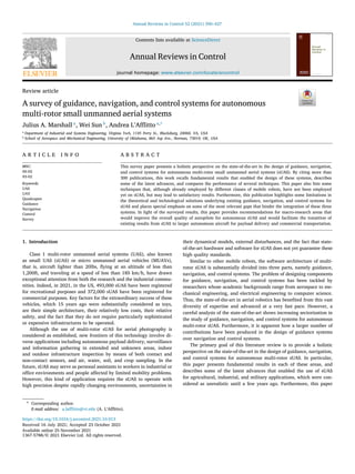
their key characteristics. Fig. 2 provides a schematic representation
of a guidance, navigation, and control system architecture for sUAS.
In this architecture, data produced by plug-in sensors, such as depth
and tracking cameras, are employed to generate occupancy maps.
Furthermore, data produced by altimeters and GNSS are merged with
data produced by the autopilot’s IMU to estimate the sUAS’ state. Some
depth and tracking cameras are able to produce reliable estimates
of the sUAS’ state as well. The occupancy maps and the estimates
on the sUAS’ state are exploited by the path planner to generate a
sequence of collision-free waypoints, and by the trajectory planner
to generate dynamically feasible reference trajectories that interpolate
these waypoints. In this architecture, the autopilot is exploited for its
4. Annual Reviews in Control 52 (2021) 390–427
393
J.A. Marshall et al.
Fig. 1. An architecture of the guidance, navigation, and control system employed on COTS autopilots for sUAS. Data produced by the onboard sensors is elaborated by the
navigation system to produce estimates of the sUAS’ state. A path planner outlines sequences of waypoints to reach user-defined goal points. In some cases, the autopilot embeds
a trajectory planner to interpolate the user-defined sequence of goal points or a subset thereof. Finally, a control law, typically linear, determines the thrust force each propeller
must exert to track the reference path or trajectory.
Fig. 2. Schematic representation of a guidance, navigation, and control system architecture for sUAS. Depth and tracking cameras or LiDARs are employed to generate occupancy
maps. Data produced by altimeters, GNSS, and the autopilot’s IMU are employed to estimate the sUAS’ state. These data are exploited by the path planner and trajectory planner.
The autopilot’s control algorithm is used to determine the thrust force each propeller must exert. Circled numbers show the order in which information flows across sensors and
algorithms. In some cases, trajectory planners, such as MPC algorithms, also produce a control input that overrides the control input computed by the autopilot.
sensors, its control algorithm, and its ability to coordinate the sUAS’
motors. In some cases, the autopilot receives the reference trajectory
for the sUAS’ position as a sequence of points and hence, the autopilot’s
control law is tasked with closely following this sequence of points. In
these cases, a trajectory planner is still necessary since, as discussed
in Section 4 below, some path planners do not produce dynamically
feasible paths. Usually, it is not possible to associate a time stamp to
each sample point of a reference trajectory sent to the autopilot. To
overcome this limitation, sampled points of the reference trajectory
can be transmitted to the autopilot at a frequency computed so that,
5. Annual Reviews in Control 52 (2021) 390–427
394
J.A. Marshall et al.
Fig. 3. Schematic representation of a guidance, navigation, and control system architecture for sUAS. The guidance, navigation, and control algorithms are executed on a single-board
computer, and the autopilot is used only for its sensors for state estimation and for its ability to coordinate the sUAS’ motors. Circled numbers show the information flow across
sensors and algorithms. In some architectures, the single-board computer is interfaced with the motors directly.
Table 3
Some commonly used COTS single-board computers for multi-rotor sUAS.
Single-board
computer
Major
Characteristics
Weight Power
consumption
Intel NUC 7i7 2–32 GB RAM,
4.2 GHz,
SSD storage
230 g 15 W
ODroid XU4 2 GB RAM, 2 GHz,
GPIO (40 Pin header)
50 g 4 A/5 V
ODroid N2+ 2–4 GB RAM, 2.4 GHz,
GPIO (40 Pin header)
200 g 2A/12V
Raspberry Pi4 2–8 GB RAM, 1.5 GHz,
GPIO (40 Pin header)
50 g 2.5 A/5 V
Nvidia
Jetson TX2
8 GB RAM, 2 GHz,
Camera support
from 256 core GPU
300 g 7–15 W
Nvidia
Jetson TX2 NX
4 GB RAM, 2 GHz,
Camera support
from 128 core GPU
90 g 5–10
VOXL Flight 4 GB RAM, 2.15 GHz,
includes Flight
Core autopilot
40 g 3–10 W
knowing the sUAS’ reference velocity, the reference trajectory is fol-
lowed at the desired speed. Alternatively, it is possible to send the
sUAS’ reference velocity, sampled over time, to the autopilot. In other
cases, the autopilot receives the desired position in the sUAS’ vertical
direction and the desired attitude in the form of discrete-time sequences
and hence, the autopilot’s control input is designed to track the desired
inner loop dynamics; for additional details, see Section 6.1 below.
Finally, in some cases, trajectory planners, such as MPC algorithms, also
produce a control input that is passed to the sUAS’ motors through the
autopilot, and the autopilot’s control system is overridden.
In several mission scenarios, the sUAS must meet user-defined spec-
ifications on the trajectory tracking error despite poor knowledge of
their payload, possible faults and failures, or strong disturbances. These
requirements are usually met by employing control laws, whose com-
plexity and computational costs exceed the capabilities of the proces-
sors installed in common COTS autopilots. Therefore, in these cases, the
control laws are computed on a single-board computer. Fig. 3 shows a
graphical representation of a guidance, navigation, and control system
architecture for sUAS, whereby path planning, trajectory planning,
localization and mapping, and control algorithms are executed on the
single-board computer. In this case, the autopilot is exploited only
for its sensors, whose data are merged with the data produced by
additional plug-in sensors, and as an interface with the sUAS’ motors.
In similar architectures, the single board computer serves as autopilot,
and COTS autopilots are not employed.
The hardware aboard sUAS is chosen according to the mission
objectives and requirements. Quadcopters employed for recreational
purposes are usually equipped with an autopilot, a relatively inex-
pensive GNSS unit, an IMU, cameras to capture aerial images, and
antennas to transmit telemetry and images in real time. Quadcopters
tasked with an autonomous indoor-only mission do not utilize GPS,
since the satellite signal is usually unreliable or unavailable, and are
usually equipped with optical flow sensors, depth and tracking cameras,
or LiDARs to determine the vehicle’s position and orientation relative to
the environment, and a single-board computer to elaborate the sensors’
data and enable autonomous operations. Quadcopters performing day-
time missions outdoors may be equipped with LiDARs, since cameras
may be blinded by strong light, and a GNSS unit. Quadcopters perform-
ing night-time missions or operating in subterranean environments,
such as caves and mines, may be equipped with LiDARs and infrared
cameras.
The required levels of precision and robustness to disturbances,
faults, failures, and uncertainties varies with the mission objectives.
For example, sUAS for recreational purposes need to guarantee sub-
meter precision and moderate robustness to minor damages. Outdoor
operations in complex environments, such as forests, may require sub-
centimeter precision, and hence are equipped with a differential GPS
(DGPS), depth and tracking cameras, and high-resolution IMUs, to
6. Annual Reviews in Control 52 (2021) 390–427
395
J.A. Marshall et al.
determine the vehicle’s position and attitude. Alternatively, if a quad-
copter operates in an indoor industrial environment, in close proximity
to untrained personnel and expensive infrastructures, sub-centimeter
precision and high levels of robustness to uncertainties in the trans-
ported payload, environmental conditions, faults, and failures are usu-
ally demanded. The required level of precision influences both the
quality of the hardware components and the expected ability of the
guidance, navigation, and control algorithms to leverage these compo-
nents and meet the desired levels of performance. This paper surveys
guidance, navigation, and control techniques for multi-rotor sUAS con-
sidering both algorithms that meet lower levels of performance and
more advanced algorithms that guarantee higher levels of precision and
robustness.
3. Equations of motion of quadcopters
Quadcopter sUAS comprise four propellers, whose spin axes are
parallel to one another, and which are connected by means of an H-
or X-shaped frame made of carbon fiber, plastic, or other material with
good stiffness and elasticity properties. The center of the frame hosts
the vehicles’ electronics, such as its single-board computer, a GNSS unit,
an IMU, antennas to receive commands and transmit telemetry in real
time, a battery, and one or multiple cameras to observe and collect data
on the environment; Fig. 4 shows a typical quadcopter.
The optical axis of these cameras is usually aligned with the bisector
of the angle between two arms of the sUAS’ frame, and this axis is
commonly chosen as the vehicle’s roll axis 𝑥body ∶ [𝑡0, ∞) → R3, where
‖𝑥body(𝑡)‖ = 1, 𝑡 ≥ 𝑡0. There is not a commonly accepted choice on
the vehicle’s yaw axis 𝑧body ∶ [𝑡0, ∞) → R3, where ‖𝑧body(𝑡)‖ = 1,
𝑡 ≥ 𝑡0, and 𝑧T
body
𝑥body(𝑡) = 0. Numerous authors, especially those
with an aeronautical background, set the yaw axis so that it points
down, whereas many other authors, especially those with an electrical
engineering or computer science background, set, without loss of gen-
erality, the yaw axis so that it points up; in this paper, the aeronautical
convention is followed. Having set the roll and yaw axes, the pitch
axis 𝑦body ∶ [𝑡0, ∞) → R3 is set so that the sUAS’ reference frame
J(⋅) ≜ {𝐴(⋅); 𝑥body(⋅), 𝑦body(⋅), 𝑧body(⋅)}, which is centered at the reference
point 𝐴 ∶ [𝑡0, ∞) → R3, is right-handed and orthonormal, that is,
𝑥×
body
(𝑡)𝑦body(𝑡) = 𝑧body(𝑡), 𝑡 ≥ 𝑡0, where (⋅)× denotes the cross-product
operator. The reference point 𝐴(⋅) is usually chosen as the vehicle’s
center of mass. However, other choices, such as the payload’s position
in the case of autonomous sUAS transporting sling payloads (Feng,
Rabbath, & Su, 2018; Schmuck & Chli, 2019a), are equally suitable.
Fig. 4 shows an orthonormal reference frame set according to the
aeronautical convention.
The sUAS’ position and attitude are captured relative to an or-
thonormal reference frame I ≜ {𝑂; 𝑋, 𝑌 , 𝑍} fixed with the Earth and
considered as inertial. Following an aerospace convention, the axes of
this reference frame can be set, for instance, so that 𝑋 points North,
𝑌 points East, and 𝑍 points down, that is, aligned with the vehicle’s
weight captured by 𝐹I
g = 𝑚𝑔𝑍, where 𝑚 > 0 denotes the sUAS’ mass
and 𝑔 > 0 denotes the gravitational acceleration. The sUAS’ mass is
usually considered as a constant; recently, the problem of modeling
and controlling sUAS, whose mass varies as a function of time due
to sudden payload dropping or a slow release of payload, has been
addressed in L’Afflitto and Mohammadi (2017). In the following, if a
vector 𝑎 ∈ R3 is expressed in the reference frame I, then this vector is
denoted by 𝑎I. Alternatively, if a vector is expressed in the reference
frame J(⋅), then no superscript is used.
In the reference frame I, the translational kinematic equation of a
quadcopter is given by
̇
𝑟I
𝐴(𝑡) = 𝑣I
𝐴(𝑡), 𝑟I
𝐴(𝑡0) = 𝑟I
𝐴,0
, 𝑡 ≥ 𝑡0, (1)
and the translational dynamic equation is given by
𝐹I
g − 𝐹I
T(𝑡) + 𝐹I
(𝑡) = 𝑚
[
̇
𝑣I
𝐴(𝑡) + ̈
𝑟I
𝐶 (𝑡)
]
, 𝑣I
𝐴(𝑡0) = 𝑣I
𝐴,0
, (2)
Fig. 4. Orthonormal reference frame centered at the sUAS’ center of mass and oriented
according to the aeronautical conventions, that is, with 𝑧body(⋅) pointing down and
𝑥body(⋅) aligned with the roll axis. Quadcopters are usually symmetric so that propellers
are placed at a distance 𝑙𝑥 from the pitch axis and 𝑙𝑦 from the roll axis.
where −𝐹T(𝑡) ≜
[
0, 0, 𝑢1(𝑡)
]T
denotes the thrust force, that is, the force
produced by the propellers that allows a quadcopter to hover, 𝐹 ∶
[𝑡0, ∞) → R3 denotes the aerodynamic forces acting on the sUAS, and
𝑟𝐶 ∶ [𝑡𝑜, ∞) → R3 denotes the position of the sUAS’ center of mass
relative to the user-defined reference point 𝐴(⋅). External disturbances
can be accounted for in the left-hand side of (2) as unknown, bounded
functions of time. Indeed, some authors embed both aerodynamic
forces and external disturbances in 𝐹I(⋅).
The orientation of the body reference frame J(⋅) relative to the
inertial reference frame I is usually captured by means of a 3-2-1
rotation sequence of implicit Tait–Bryan angles so that
[
𝑥I
body
(𝑡), 𝑦I
body
(𝑡), 𝑧I
body
(𝑡)
]
= 𝑅(𝜙(𝑡), 𝜃(𝑡), 𝜓(𝑡)), 𝑡 ≥ 𝑡0,
where
𝑅(𝜙, 𝜃, 𝜓) ≜
⎡
⎢
⎢
⎣
cos 𝜓 − sin 𝜓 0
sin 𝜓 cos 𝜓 0
0 0 1
⎤
⎥
⎥
⎦
⎡
⎢
⎢
⎣
cos 𝜃 0 sin 𝜃
0 1 0
− sin 𝜃 0 cos 𝜃
⎤
⎥
⎥
⎦
×
⎡
⎢
⎢
⎣
1 0 0
0 cos 𝜙 − sin 𝜙
0 sin 𝜙 cos 𝜙
⎤
⎥
⎥
⎦
,
(𝜙, 𝜃, 𝜓) ∈ [0, 2𝜋) ×
(
−
𝜋
2
,
𝜋
2
)
× [0, 2𝜋),
𝜙 ∶ [𝑡0, ∞) → [0, 2𝜋) denotes the roll angle, 𝜃 ∶ [𝑡0, ∞) → (−𝜋
2
, 𝜋
2
) denotes
the pitch angle, and 𝜓 ∶ [𝑡0, ∞) → [0, 2𝜋) denotes the yaw angle. In this
case, the rotational kinematic equation of a quadcopter is given by
⎡
⎢
⎢
⎣
̇
𝜙(𝑡)
̇
𝜃(𝑡)
̇
𝜓(𝑡)
⎤
⎥
⎥
⎦
= 𝛤(𝜙(𝑡), 𝜃(𝑡))𝜔(𝑡),
⎡
⎢
⎢
⎣
𝜙(𝑡0)
𝜃(𝑡0)
𝜓(𝑡0)
⎤
⎥
⎥
⎦
=
⎡
⎢
⎢
⎣
𝜙0
𝜃0
𝜓0
⎤
⎥
⎥
⎦
, (3)
where
𝛤(𝜙, 𝜃) ≜
⎡
⎢
⎢
⎣
1 sin 𝜙 tan 𝜃 cos 𝜙 tan 𝜃
0 cos 𝜙 − sin 𝜙
0 sin 𝜙 sec 𝜃 cos 𝜙 sec 𝜃
⎤
⎥
⎥
⎦
, (𝜙, 𝜃) ∈ [0, 2𝜋) ×
(
−
𝜋
2
,
𝜋
2
)
.
The Tait–Bryan angles, like any attitude representation system based on
three independent parameters, are limited by the presence of a singular
configuration, that is, a configuration wherein the attitude representa-
tion is not unique, and a finite angular velocity would imply an infinite
7. Annual Reviews in Control 52 (2021) 390–427
396
J.A. Marshall et al.
time derivative of the angles capturing the vehicle’s orientation. In the
case of a 3-2-1 rotation sequence, this singular configuration is attained
for |𝜃(𝑡)| = 𝜋
2
, 𝑡 ≥ 𝑡0. To overcome this problem, some authors employ
attitude representation system based on four parameters, such as the
Euler parameters, which are commonly referred to as quaternions. The
rotational dynamic equation of a quadcopter, whose frame is modeled
as a rigid body, whose payload is rigidly attached to the vehicle, and
whose propellers are modeled as thin spinning discs, is given by
𝑀T(𝑡) + 𝑀g(𝑟𝐶 (𝑡), 𝜙(𝑡), 𝜃(𝑡)) + 𝑀(𝑡)
= 𝑚𝑟×
𝐶
(𝑡)
[
̇
𝑣𝐴(𝑡) + 𝜔×
(𝑡)𝑣𝐴(𝑡)
]
+ 𝐼 ̇
𝜔(𝑡)
+ 𝜔×
(𝑡)𝐼𝜔(𝑡) + 𝐼P
4
∑
𝑖=1
⎡
⎢
⎢
⎣
0
0
̇
𝛺P,𝑖(𝑡)
⎤
⎥
⎥
⎦
+ 𝜔×
(𝑡)𝐼P
4
∑
𝑖=1
⎡
⎢
⎢
⎣
0
0
𝛺P,𝑖(𝑡)
⎤
⎥
⎥
⎦
,
𝜔(𝑡0) = 𝜔0, 𝑡 ≥ 𝑡0, (4)
where 𝑀T(𝑡) = [𝑢2(𝑡), 𝑢3(𝑡), 𝑢4(𝑡)]T denotes the moment of the forces
induced by the propellers, 𝑀g(𝑟𝐶 , 𝜙, 𝜃) ≜ 𝑟×
𝐶
𝐹I
g (𝜙, 𝜃), (𝑟𝐶 , 𝜙, 𝜃) ∈ R3 ×
[0, 2𝜋) ×
(
−𝜋
2
, 𝜋
2
)
, denotes the moment of the quadcopter’s weight with
respect to 𝐴,
𝐹I
g (𝜙, 𝜃) = 𝑚𝑔[− sin(𝜃), cos(𝜃) sin(𝜙), cos(𝜃) cos(𝜙)]T
,
(𝜙, 𝜃) ∈ [0, 2𝜋) ×
(
−
𝜋
2
,
𝜋
2
)
,
𝑀 ∶ [𝑡0, ∞) → R3 denotes the moment of the aerodynamic forces with
respect to 𝐴(⋅), 𝐼 ∈ R3×3 denotes the symmetric positive-definite matrix
of inertia of the sUAS relative to 𝐴(⋅), excluding the propellers, 𝐼P ∈
R3×3 denotes the symmetric positive-definite matrix of inertia of each
propeller relative to 𝐴(⋅), and 𝛺P,𝑖 ∶ [𝑡0, ∞) → R, 𝑖 = 1, … , 4, denotes
the angular velocity of the 𝑖th propeller. The terms 𝐼P
∑4
𝑖=1[0, 0, ̇
𝛺𝑃𝑖
(𝑡)]T,
𝑡 ≥ 𝑡0, and 𝜔×(𝑡)𝐼P
∑4
𝑖=1[0, 0, 𝛺𝑃𝑖
(𝑡)]T denote the inertial counter-torque
and the gyroscopic effect, respectively. It is common practice to assume
that the sUAS’ axes are principal axes of inertia and, hence, the matrix
𝐼 is usually considered as diagonal, and its entries are denoted by 𝐼𝑥,
𝐼𝑦, and 𝐼𝑧 > 0. External disturbances can be accounted for in the left-
hand side of (4) as unknown, bounded functions of time. Indeed, some
authors embed both aerodynamic forces and external disturbances in
𝑀(⋅).
In the following, we denote the equations of motion (1)–(4) by
̇
𝑥(𝑡) = 𝑓(𝑡, 𝑥(𝑡)) + 𝐺(𝑥(𝑡))𝑢(𝑡), 𝑥(𝑡0) = 𝑥0, 𝑡 ≥ 𝑡0, (5)
where 𝑥(𝑡) ≜
[
𝑞T(𝑡), 𝑞T
dot
(𝑡)
]T
, 𝑞(𝑡) =
[(
𝑟I
𝐴
(𝑡)
)T
, 𝜙(𝑡), 𝜃(𝑡), 𝜓(𝑡)
]T
de-
notes the vector of independent generalized coordinates, and 𝑞dot(𝑡) ≜
[(
̇
𝑟I
𝐴
(𝑡)
)T
, 𝜔T(𝑡)
]T
denotes the vector of quasi-velocities, 𝑢(𝑡) ≜
[𝑢1(𝑡), 𝑢2(𝑡), 𝑢3(𝑡), 𝑢4(𝑡)]T denotes the control vector; assuming, for brevity,
that 𝑟𝐶 (𝑡) ≡ 0, 𝑡 ≥ 𝑡0, and 𝐼P = 03×3, it follows from (1)–(4) that
𝑓(𝑡, 𝑥) ≜
[
(
𝑣I
𝐴
)T
, 𝑔𝑍 +
(
𝐹I
(𝑡)
)T
, 𝜔T
𝛤T
(𝜙, 𝜃),
(
𝑀(𝑡) − 𝜔×
𝐼𝜔
)T
𝐼−T
]T
,
𝐺(𝑥) ≜
⎡
⎢
⎢
⎢
⎢
⎣
05×1 05×3
𝑚−1 01×3
03×1 03×3
03×1 𝐼−1
⎤
⎥
⎥
⎥
⎥
⎦
,
for all (𝑡, 𝑥) ∈ [𝑡0, ∞) ×
(
R3 × [0, 2𝜋) ×
(
−𝜋
2
, 𝜋
2
)
× [0, 2𝜋) × R6
)
, where
0𝑛×𝑚 denotes the zero matrix in R𝑛×𝑚. The control vector 𝑢(⋅) comprises
the third component of the thrust force 𝐹T(⋅) and the moment of the
forces induced by the propellers 𝑀T(⋅). It is possible to verify that
⎡
⎢
⎢
⎢
⎢
⎣
𝑢1(𝑡)
𝑢2(𝑡)
𝑢3(𝑡)
𝑢4(𝑡)
⎤
⎥
⎥
⎥
⎥
⎦
=
⎡
⎢
⎢
⎢
⎢
⎣
1 1 1 1
−𝑙𝑦 𝑙𝑦 −𝑙𝑦 𝑙𝑦
𝑙𝑥 −𝑙𝑥 −𝑙𝑥 𝑙𝑥
−𝑐T𝑙 −𝑐T𝑙 𝑐T𝑙 𝑐T𝑙
⎤
⎥
⎥
⎥
⎥
⎦
⎡
⎢
⎢
⎢
⎢
⎣
𝑇1(𝑡)
𝑇2(𝑡)
𝑇3(𝑡)
𝑇4(𝑡)
⎤
⎥
⎥
⎥
⎥
⎦
, 𝑡 ≥ 𝑡0, (6)
where 𝑇𝑖 ∶ [𝑡0, ∞) → R, 𝑖 = 1, … , 4, denotes the component of the force
produced by the 𝑖th propeller along the −𝑧body(⋅) axis of the reference
frame J(⋅), 𝑙𝑥 > 0 denotes the distance of the sUAS’ propellers from the
𝑥body(⋅) axis, 𝑙𝑦 > 0 denotes the distance of the sUAS’ propellers from
the 𝑦body(⋅) axis, 𝑙 ≜
√
𝑙2
𝑥 + 𝑙2
𝑦, and 𝑐T > 0 denotes the propellers’ drag
coefficient. The thrust force generated by the 𝑖th propeller is related to
the propeller’s angular velocity by
𝑇𝑖(𝑡) = 𝑘𝛺2
P,𝑖(𝑡), 𝑖 = 1, … , 4, 𝑡 ≥ 𝑡0, (7)
where 𝑘 > 0 is usually determined experimentally. Some authors
account also for the motors’ dynamics while formulating the sUAS’
equations of motion.
It follows from (5) that a quadcopter’s equilibrium condition is
attained by hovering at some constant altitude and with some constant
yaw angle. It is common practice to design quadcopters so that their
thrust-to-weight ratio is near 2-to-1. Thus, small rotations about the
pitch or roll axes lead to rapid translations along the inertial horizontal
plane. For these reasons, and since sUAS are seldom tasked with
aggressive maneuvers, it is common practice to consider the linearized
equations of motion of a quadcopter, while designing guidance, naviga-
tion, and control systems for sUAS. Linearizing (5) about a user-defined
equilibrium condition, the sUAS’ dynamics can be approximated by
̇
̃
𝑥(𝑡) = ̃
𝐴̃
𝑥(𝑡) + ̃
𝐵 ̃
𝑢(𝑡), ̃
𝑥(𝑡0) = ̃
𝑥0, 𝑡 ≥ 𝑡0, (8)
where ̃
𝑥(𝑡) ≜
[
𝑞T(𝑡), ̇
𝑞T(𝑡)
]T
denotes the linearized state vector, ̃
𝑢(𝑡) ≜
[𝑢1(𝑡) − 𝑚𝑔, 𝑢2(𝑡), 𝑢3(𝑡), 𝑢4(𝑡)]T, ̃
𝐴 ≜
⎡
⎢
⎢
⎢
⎢
⎣
06×3 06×2 06×1 𝟏6
02×3
[
0 −𝑔
𝑔 0
]
02×1 02×6
04×3 04×2 04×1 04×6
⎤
⎥
⎥
⎥
⎥
⎦
∈
R12×12, 𝟏𝑛 denotes the identity matrix in R𝑛×𝑛, and ̃
𝐵 ≜
[
08×4
diag(𝑚−1, 𝐼−1
𝑥 , 𝐼−1
𝑦 , 𝐼−1
𝑧 )
]
∈ R12×4.
The guidance, navigation, and control problems for multi-rotor
sUAS are usually solved numerically in discrete time. Thus, the
continuous-time linearized equations of motion of multi-rotor sUAS
can be recast in a discrete-time form by employing, for instance, the
zero-order hold approach so that (8) is discretized as
̂
𝑥(𝑡0 + (𝑖 + 1)𝛥𝑇 ) = 𝐴̂
𝑥(𝑡0 + 𝑖𝛥𝑇 ) + 𝐵 ̂
𝑢(𝑡0 + 𝑖𝛥𝑇 ),
8. Annual Reviews in Control 52 (2021) 390–427
397
J.A. Marshall et al.
̂
𝑥(𝑡0) = ̃
𝑥0, 𝑖 ∈ N ∪ {0}, (9)
where 𝐴 = 𝑒
̃
𝐴𝛥𝑇 , 𝐵 = ∫
𝛥𝑇
0 𝑒
̃
𝐴𝜎d𝜎 ̃
𝐵, and 𝛥𝑇 > 0 denotes the time step.
In some cases, it is more convenient to set the boundary conditions
on the sUAS’ position and translational velocity both at 𝑡0 and at the
time instant 𝑡0 + 𝑛t𝛥𝑇 , where 𝑛t ∈ N is user-defined; in these cases,
to accommodate 12 boundary conditions on the 12 states comprised in
̂
𝑥(⋅), the boundary conditions on the sUAS’ attitude and angular velocity
cannot be imposed arbitrarily.
4. Guidance systems for autonomous multi-rotor sUAS
Guidance can be described as the determination of the vehicle’s
reference path or trajectory that should be closely followed by a user-
defined reference point on the vehicle. Path planning aims at outlin-
ing a collision-free sequence of waypoints from the vehicle’s current
position to the goal set. Trajectory planning aims at outlining a con-
tinuous collision-free curve, parameterized by time, compatibly with
user-defined constraints such as the need to avoid saturation of the
actuators and the need not to exceed the vehicles’ flight envelope.
Usually, trajectory planning systems for sUAS are also aimed at defining
the sUAS’ reference yaw angle so that the onboard sensors or the
payload are steered in a specific direction. For instance, it is common
practice to steer the sUAS’ longitudinal axis so that the next waypoint is
always in the field of view of the sUAS’ cameras. Finally, in numerous
cases, the trajectory planning system is tasked with defining the sUAS’
reference angular position and angular velocity, and hence, with pro-
ducing reference trajectories for the sUAS by steering the thrust force
in some direction compatibly with the sUAS’ rotational dynamics.
This section surveys path planning and trajectory planning tech-
niques by recalling both classical approaches and recent learning-based
methods. Thus far, the path planning and the trajectory planning
problems have been largely addressed separately since some guidance
systems embed either a path planner or a trajectory planner. How-
ever, addressing these two problems separately may produce several
challenges. Indeed, numerous path planners do not account for the
sUAS’ dynamics, and if only a path planner is employed, then following
dynamically unfeasible reference trajectories stresses the performance
of the control system; for additional details, see Section 6.1 below.
Numerous trajectory planners operate on sets characterized by strong
properties, such as convexity, since convexity of the cost function over
the constraint set is a sufficient condition on the existence of a unique
solution for optimization-based planners; for additional details, see Sec-
tion 5.5 below. However, operating on convex sets is a limiting factor in
most problems of practical interest. Indeed, if only a trajectory planner
is employed, and this planner operates on convex sets only, then, it
may be impossible to find a reference trajectory leading the sUAS
from its current location to the goal set. In many cases, path planners
and trajectory planners are employed sequentially by exploiting the
ability of most path planners to produce a sequence of waypoints from
the sUAS’ current location to the goal set in the presence of complex
constraints and then, by employing trajectory planners to interpolate
multiple waypoints produced by the path planner. Recently, some effort
has been made to integrate path and trajectory planners, and this
section also surveys approaches to merging path and trajectory plan-
ning systems. In this section, we also survey some of the most notable
techniques employed to generate reference paths and trajectories for
swarms of sUAS. Finally, we survey two relatively new areas, namely
guidance systems for autonomous sUAS operating in a tactical manner
to support operations of ground troops and law enforcement agencies
and guidance systems for autonomous sUAS flying as fast as possible.
4.1. Path planners for sUAS
In the following, we present multiple path planning techniques
grouped as optimization-based and non-optimization-based methods,
local and global methods, roadmap methods, exact or approximate cell
decomposition methods, reactive methods, methods based on motion
primitives, bio-inspired approaches, and learning-based methods; these
classifications are not mutually exclusive. Furthermore, we discuss
a relatively under-explored class of path planners, that is, planners
designed to guarantee stability of the vehicle. Other classifications of
path planning methods for mobile robots, such as offline and online
methods, are not discussed, since the totality of guidance systems
for multi-rotor sUAS currently involve only online path planners. Key
features of the most relevant path planning techniques surveyed in
this paper are listed in Table 4. Presently, COTS autopilots, such as
those listed in Table 1, implement relatively simple path planning
algorithms; for instance, ArduPilot allows to implement the Dijkstra’s
algorithm. However, more complex algorithms, including the majority
of those surveyed in the following, need to be executed on single-board
computers such as those listed in Table 3.
Unless stated otherwise, in the following, the path planning problem
is considered as three-dimensional. Exploiting the vertical direction
allows to explore more solutions to the path planning problem than
solvers designed for two-dimensional problems only. However, in gen-
eral, exploring the three-dimensional space implies increased computa-
tional costs. Furthermore, increasing the sUAS’ altitude usually depletes
the batteries more rapidly.
4.1.1. Optimization and non-optimization based methods
Non-optimization-based path planning methods are merely con-
cerned with the problem of finding a reference path from the sUAS’
current location to the goal set, which is feasible according to the
information on the environment available at the time the planning pro-
cess is initiated. Among non-optimization-based path planning methods
is the rapidly exploring random tree method (𝑅𝑅𝑇 ) (Saravanakumar
9. Annual Reviews in Control 52 (2021) 390–427
398
J.A. Marshall et al.
Table 4
Some of the most common path planning methods for sUAS, some of their key features, and selected references applying these methods to multi-rotor sUAS. The majority of
existing techniques, or variations thereof, produce reference paths that minimize some cost function. Relatively few methods are global, that is, search the entire space in which
the sUAS operates; local planning techniques need to be applied on multiple partitions of the map. Few techniques are complete and hence, allow to find a reference path from
any initial position to any goal set. In some cases, a complete solution may be attained by applying a path planning technique to multiple adjacent subsets of the free space,
which meet some specific criteria such as convexity.
Algorithm Optimal Global Complete Cell decomposition Ref.
𝐀∗
& variations ✓ ✓ ✓ ✓ Zhao, Zhang, and Zhao (2020)
𝐃∗
& variations ✓ ✓ ✓ ✓ Koenig and Likhachev (2002, 2005)
Disjunctive convex programming ✓ Through iterations Blackmore, Ono, and Williams (2011)
Maneuver automata ✓ Frazzoli, Dahleh, and Feron (1999), Schouwenaars,
Mettler, Feron, and How (2004)
Mixed integer linear program ✓ Through iterations Babel (2019)
Mixed integer quadr. program ✓ Through iterations Tordesillas, Lopez, and How (2019)
Motion primitives ✓ Yadav and Tanner (2020), Zhou, Gao, Wang, Liu,
and Shen (2019a)
Potential field ✓ Through iterations Woods and La (2019)
Probabilistic roadmap ✓ ✓ ✓ Xu, Deng, and Shimada (2021)
RRT & variations 𝑅𝑅𝑇 ∗
✓ ✓ ✓ Karaman and Frazzoli (2011), Saravanakumar,
Kaviyarasu, and Ashly Jasmine (2021)
Meng, Pawar, Kay, and Li (2018)
Wavefront algorithm ✓ ✓ ✓ ✓ Hebecker, Buchholz, and Ortmeier (2015)
et al., 2021), which is still considered as one of the fastest path plan-
ning methods, compatible with the quality of the underlying random
number generator (Noreen, Khan, Ryu, Doh, & Habib, 2018), and the
probabilistic roadmap method (Xu et al., 2021), which guarantees low
computational costs.
It is rare that a satisfactory path is merely collision-free since multi-
ple additional criteria such as minimum time or minimum distance, to
name two of the most common metrics, must be met. Optimization-
based methods are designed to meet both collision avoidance con-
straints, the requirement of maximizing some reward function or,
equivalently, of minimizing some cost function. Among the optimiza-
tion methods, 𝐴∗ (Zhao et al., 2020), which is widely used for its fast
convergence and low time complexity (Primatesta, Guglieri, & Rizzo,
2019), 𝐷∗, and 𝐷∗-lite (Koenig & Likhachev, 2002, 2005), which are
suitable for highly dynamic environments, mixed integer quadratic
programming (Tordesillas et al., 2019), 𝑅𝑅𝑇 ∗ (Karaman & Frazzoli,
2011), informed 𝑅𝑅𝑇 ∗ (Meng et al., 2018), which guarantees faster
convergence than conventional 𝑅𝑅𝑇 ∗, mixed integer linear program-
ming (Babel, 2019), and disjunctive convex programming (Blackmore
et al., 2011).
Algorithm 1 provides an implementation of the 𝐴∗ technique to
reach the goal node 𝑛g from the initial node 𝑛0 through a weighted graph.
In path planning applications for sUAS, this graph can be provided,
for instance, by creating partitions of a map that are not occupied by
obstacles, setting a point for each partition as a node of the graph,
and setting the weights on the edges of the graph as the distance
between nodes. Thus, the 𝐴∗ algorithm provides a sequence of nodes
∗ connecting 𝑛0 to 𝑛g that minimizes the cost function
𝑓(𝑛0, 𝑛g) ≜ 𝑔(𝑛0, 𝑛c) + ℎ(𝑛𝑐, 𝑛g), (𝑛0, 𝑛c, 𝑛g) ∈ × × , (10)
where the cost-to-come function 𝑔 ∶ × → R denotes the cost of
reaching the current node 𝑛c from 𝑛0, the heuristic function ℎ ∶ × →
R denotes an underestimate of the cost of reaching the node 𝑛g from 𝑛c,
and denotes the set of nodes of the graph. As it progresses through
the graph, the 𝐴∗ algorithm constructs ∗ by investigating all the
nodes adjacent to the current node 𝑛c, selecting the node that provides
the lowest 𝑓(𝑛0, 𝑛g), and finally tracing back ∗ from 𝑛g to 𝑛0.
4.1.2. Global and local methods
Global methods provide a reference path by searching the entire
space in which the sUAS operates, whereas local methods provide
reference paths to subsets of the goal set or waypoints located in subsets
of the search space that meet some specific criteria such as convexity.
Many of the aforementioned techniques, such as 𝑅𝑅𝑇 , 𝐴∗, or 𝐷∗-lite,
are global methods. Among local path planning methods applied to
Algorithm 1: 𝐴∗ algorithm for returning best path relative to the
cost function 𝑓(⋅, ⋅) and the cost-to-come function 𝑔(⋅, ⋅).
Result: ∗: nodes of the shortest path from 𝑛0 to 𝑛g.
Create empty priority queue ;
𝑛0 = Current node ;
Insert 𝑛0 → ;
while is not empty do
Set current node 𝑛 to first node in ;
if 𝑛 = 𝑛g then
Break while and Reconstruct Path( ∗) ;
end
Remove 𝑛 from ;
for All 𝑛′ adjacent to 𝑛 in do
if 𝑛′ ∉ then
Insert 𝑛′ → ;
In , set pointer of 𝑛′ towards 𝑛 ;
end
else if 𝑔(⋅, 𝑛′) > 𝑔(𝑛0, 𝑛) + 𝑔(𝑛, 𝑛′) then
Modify by setting pointer of 𝑛′ towards 𝑛 ;
Update 𝑛′ → ;
end
end
end
Reconstruct Path( ∗): Trace the pointers from 𝑛g back to 𝑛0;
sUAS, we recall the wavefront algorithm (Hebecker et al., 2015), and
some versions of the potential field method (Woods & La, 2019) that
require partitioning the search space into convex subsets. Restricting
potential fields on convex sets allows to avoid multiple, undesired, local
minima where the search algorithm may converge.
In general, global path planners are preferred over local path plan-
ners since a path planner’s role is to coarsely outline a way for the sUAS
to complete the given mission, whereas the trajectory planner locally
refines the path and accounts for the vehicle’s dynamic constraints. A
notable exception to this consideration is given by the use of potential
field methods to locally coordinate swarms of sUAS (Zhou & Schwager,
2016). However, the use of local repulsive fields to avoid collisions
among formation agents and with obstacles alongside the use of attrac-
tive fields to draw the swarm to the goal set may lead to undesired
conditions of local equilibria.
10. Annual Reviews in Control 52 (2021) 390–427
399
J.A. Marshall et al.
4.1.3. Roadmap methods
Roadmap approaches to the path planning problem for sUAS include
the visibility graph method (Blasi, D’Amato, Mattei, & Notaro, 2020),
which is usually implemented in static environments, Voronoi dia-
grams (Baek, Han, & Han, 2020), which are easy to implement, but are
also inefficient in high dimensions because they require complex data
structures and long pre-processing times, and power diagrams (Auren-
hammer, 1987), which provide a generalization of Voronoi diagrams.
To the authors’ knowledge, alternative roadmap approaches, such as
freeway nets (Latombe, 2012, Ch. 4) and silhouettes (LaValle, 2006,
Ch. 6), which have been employed for other classes of mobile robots,
such as autonomous ground vehicles operating indoors, have not been
applied yet to the path planning problem for sUAS. Although current
implementations of freeway nets concern two-dimensional problems,
this technique provides a good solution to the path planning problem
in structured environments, such as manufacturing plants or towns
with grid street plans, where large safety margins are preferable and
excursions in the vertical direction are discouraged. Thus, the use of
freeway nets may be worthwhile being investigated. For the complexity
of their construction, silhouettes may be particularly demanding for
computers on current sUAS.
4.1.4. Decomposition methods
Decomposition methods consist in partitioning a map of the envi-
ronment and outlining paths that join some points deemed as represen-
tatives of these partitions. Some path planning techniques, such as the
visibility graph, Voronoi diagrams, 𝐴∗, and 𝐷∗ are cell decomposition
methods. An example of a path planning method that is not based on
cell decomposition is the potential field method (Latombe, 2012, Ch.
7).
In general, decomposition methods are classified in exact and ap-
proximate methods. Exact cell decomposition methods, such as the
Schwartz and Sharir method (Schwartz & Sharir, 1983) and the Canny
method (Canny, 1988), operate over partitions of the free space, whose
union is equal to the space perceived as free by the onboard naviga-
tion system. All cell decomposition methods are global path planning
techniques and exact methods are more computationally onerous, but
complete, that is, are guaranteed to provide a feasible path. Approxi-
mate cell decomposition methods, such as grid-based methods (Galceran
& Carreras, 2013) and the circle packing method (Thurston, 1979),
operate over partitions of the free space whose union is a subset of
the free space. To the authors’ knowledge, although these techniques
were successfully implemented on relatively slow mobile ground robots
operating indoors, neither the Schwartz and Sharir method nor the
Canny method have been applied to sUAS since their computational
cost may be overly large for current single-board computers.
4.1.5. Reactive path planning methods
The path planning methods presented thus far assume that a map
of the environment is known at the time the planning algorithm is
executed. Dynamic obstacles or newly detected obstacles are accounted
for by executing the path planning algorithm at a frequency that is
equal to, or, at least, similar to the frequency at which obstacle maps
are produced. However, in densely occupied environments, creating
consistent maps at a high speed may be challenging. If a map of
the environment is incomplete, then some authors consider unknown
areas as occupied by obstacles (Oleynikova et al., 2020), whereas
other authors consider these areas as unoccupied (Han, Gao, Zhou, &
Shen, 2019). The former approach is more cautious and requires to
re-plan the reference path higher frequencies. The latter approach is
less cautious and requires the mapping and path planning algorithms
to be fast; for additional details on mapping algorithms for sUAS, see
Section 5.4 below. Reactive methods provide an alternative approach
to these path planners that require a global, consistent map of the
environment.
Given a reference path leading the sUAS to the goal set, reactive path
planning methods locally modify the reference path to avoid constraints
that were unknown at the time the original reference path was outlined.
Re-planning can be performed by executing any of the path planning
techniques surveyed thus far in neighborhoods of the sUAS that are
sufficiently large to comprise a point of the original reference path,
known as aiming point, which is past those obstacles that are about
to be intercepted. A key advantage in the use of reactive methods
is that they do not need global, consistent maps of the environment,
but only local obstacle maps. Therefore, these algorithms are useful
for those applications, wherein the sUAS is required to reach a goal
set, and a consistent map of the environment traversed is unnecessary.
Examples of reactive path planning methods for sUAS are presented
in Berger, Rudol, Wzorek, and Kleiner (2016), Choi, Kim, and Hwang
(2011), Tripathi, Raja, and Padhi (2014) and Viquerat, Blackhall, Reid,
Sukkarieh, and Brooker (2008).
4.1.6. Motion primitive libraries and motion automata
Some path planning techniques for sUAS consist of selecting in
real time some pre-computed motion primitives, that is, libraries of
maneuvers such as hover, ascent and descent at a given velocity,
forward flight at a given pitch angle, and turns at a given roll angle
(Zhou et al., 2019a); a schematic representation of path planning
techniques based on the use of motion primitives is provided in Fig. 5.
Some path planning techniques consist in devising behavior primi-
tives, that is, collections of motion primitives to perform given tasks
or subtasks (Engebraaten, Moen, Yakimenko, & Glette, 2020). Upon
constructing motion primitives, if the sUAS is modeled as a point mass,
then by employing motion primitives, the path planning problem is
cast in six-dimensions. Alternatively, if both the translational and the
rotational dynamics are considered, then the path planning problem is
cast in twelve-dimensions.
Path planners based on motion primitives are advantageous because
finding the reference path reduces to searching sparse graphs, whose
nodes are given by the motion primitives, and hence, are usually fast.
Additional advantages of path planners based on motion primitives
involve their ability to account for the sUAS’ dynamics, and hence, pro-
duce feasible paths, incorporate a variety of constraints, and estimate
the time needed to follow the reference path. However, irrespective
of the technique used to search the graph, these methods are not
necessarily complete since there may not exist a combination of motion
primitives leading the sUAS to the goal set. To overcome this limitation,
the authors in Yadav and Tanner (2020) use motion primitives to
generate local goals and employ a receding horizon control framework
to generate feasible trajectories.
Similar to the notion of motion primitives is the one of maneuver au-
tomata. For instance, in Frazzoli et al. (1999), the set of trim conditions
and maneuvers generate a cost-to-go map. The reference path is then
chosen by a search algorithm over this map; maneuvers falling between
the pre-computed values are deduced via interpolation. Similarly, the
authors in Schouwenaars et al. (2004) employ the receding horizon
control approach to search maneuver automata and hence, to search
spaces of dynamically feasible paths over a predefined time horizon.
4.1.7. Bio-inspired methods
Bio-inspired path planning algorithms provide a recent trend in
aerial robotics (Pehlivanoglu, 2012; Yang, Fang, & Li, 2016). Some
of these methods, such as evolutionary algorithms, allow to solve non-
deterministic polynomial-time-hard (NP-hard) multi-objective path
planning problems, but suffer from high time complexity. Alternative
bio-inspired path planning algorithms, such as those based on neural
networks, require training with given data (de Souza, Marcato, de
Aguiar, Juca, & Teixeira, 2019) and hence, may not be suitable for
complicated missions. In general, the computational cost of bio-inspired
path planning algorithms, such as evolutionary algorithms, still provide
a challenge to real-time path planning problems in three-dimensional
environments (Yang, Qi, et al., 2016).
11. Annual Reviews in Control 52 (2021) 390–427
400
J.A. Marshall et al.
Fig. 5. An approach to path planning, which allows to account for the sUAS’ dynamics, consists in generating libraries of 𝑛 dynamically feasible trajectories off-line and storing
these libraries on the sUAS’ onboard computer. Each of these trajectories is associated with a cost index, such as the path length or the travel time. Casting each motion primitive
as the arc of a weighted graph, search algorithms can be employed to determine sequences of dynamically feasible trajectories that lead the sUAS to its goal set. This approach
was employed, for instance, in Han, Zhang, Pan, Xu, and Gao (2020) and Zhou, Gao, Wang, Liu, and Shen (2019b).
4.1.8. Learning-based methods
Machine learning methods such as reinforcement learning and deep
learning have been utilized in recent years to improve the sampling-
based path planning methods such as 𝑅𝑅𝑇 . For instance, the sam-
pling distribution in the sampling-based path planners can be learned
through various machine learning methods such as a conditional vari-
ational autoencoder (Sohn, Lee, & Yan, 2015) or a policy search-based
method (Zhang, Huh, & Lee, 2018). Alternatively, an incremental
sampling-based motion planning algorithm based on 𝑅𝑅𝑇 is presented
in Li, Cui, Li, and Xu (2018), where the cost function is predicted by a
neural network. Finally, an optimal path planning algorithm based on
a convolutional neural network (CNN) and 𝑅𝑅𝑇 ⋆ is proposed in Wang,
Chi, Li, Wang, and Meng (2020).
Some of these learning-based techniques have already been applied
to path planning to sUAS. For instance, the conditional variational
autoencoder has been recently employed in Xia et al. (2020). Only
recently, deep neural networks and some deep reinforcement learning
techniques, such as Deep Q-network (DQN) (Lv, Zhang, Ding, & Wang,
2019; Yan, Xiang, & Wang, 2020), have been employed to plan paths
for sUAS. A DQN-based algorithm for optimal waypoint planning is
presented in Eslamiat, Li, Wang, Sanyal, and Qiu (2019) and combined
with optimal trajectory generation through waypoints and nonlinear
tracking control for real-time operation of sUAS.
4.1.9. Stable path planners for sUAS
A relatively under-explored class of path planners comprises those
techniques explicitly designed to account for the vehicle’s stability
properties. Indeed, the majority of path planning techniques are merely
concerned with the problem of leading the vehicle to the goal set, while
avoiding constraints. However, in the presence of dynamic constraints,
sudden maneuvers may induce some instability.
Among the few methods for stable path planning known to the
authors, it is worthwhile to recall (Kang et al., 2015), where the path
planning problem is addressed by employing a genetic algorithm, and
Norouzi, De Bruijn, and Miró (2012), which leverages the vehicle’s
dynamics. The use of motion primitive libraries appears a promising
solution to the stable path planning problem. Indeed, motion primi-
tives can be produced by applying some technique framed within the
context of control theory, such as, for instance, one of the control
laws surveyed in Section 6 below, to a suitable dynamical model of
the sUAS, such as, for instance, (1) and (2), (5), (8), or (9). Since
these techniques guarantee the stability of the controlled sUAS, this
approach can provide a suitable framework for stable path planning,
and the control input associated with the chosen motion primitive
can be employed to directly regulate the sUAS. A potential limitation
of this approach, however, is given by the fact that instabilities may
be generated by switching across stable motion primitives and their
associated control inputs (Liberzon, 2003). A solution to the problem of
instabilities induced by switching mechanisms consists in finding some
lower bound on the dwell time, that is, the minimum time between two
consecutive switches across motion primitives.
4.2. Trajectory planners for sUAS
The large majority of mission planning problems involving sUAS are
characterized by multiple constraints, such as saturation of the control
input, which are intrinsically tied with the vehicle’s dynamics. In
these cases, analytical solutions to the trajectory planning problem are
usually impossible to find, and numerical techniques must be employed
to determine feasible reference trajectories. The trajectory planning
problem becomes further challenging for sUAS operating in unknown,
dynamic, or unstructured environments since low computational times
and high precision are required, while these vehicles’ communication
capabilities are too limited to compute feasible trajectories in real
time off-board. Presently, COTS autopilots, such as those listed in Ta-
ble 1, could implement simple trajectory planners, such as linear MPC
laws. However, in general, trajectory planning algorithms need to be
executed on single-board computers such as those listed in Table 3. Ad-
ditionally, despite the very latest advances in the design and production
of single-board computers for small mobile robots, the computational
capabilities of existing sUAS are too low to implement complex solvers.
Therefore, the problem of computing realistic reference trajectories at
a high speed and in complex environments is still considered as open.
Thus far, the trajectory planning problem has been substantially
addressed from a control-theoretic perspective by considering a plant
model, which is sufficiently representative of the sUAS’ dynamics, and
then finding a control input that allows the sUAS to reach the goal
set, while meeting collision avoidance constraints (see Sections 5.4
and 5.5 below), constraints on the control input, and user-defined
constraints on the flight envelope. Applying this approach, the state
of the plant model associated with this control input is considered as
the reference trajectory. Table 5 summarized some of the results on
trajectory planning for sUAS surveyed in this section and highlights
some of their key properties.
12. Annual Reviews in Control 52 (2021) 390–427
401
J.A. Marshall et al.
Table 5
Some of the most common trajectory planning methods for sUAS, some of their most remarkable properties, such as optimality and compatibility with COTS single-board computers
for sUAS, and selected recent publications.
Algorithm Optimal Real-Time Notes Ref.
MPC ✓ ✓ Very popular Koo, Kim, and Suk (2015), Prodan et al. (2013)
Kamel, Burri, and Siegwart (2017), Tang, Wang,
Liu, and Wang (2021)
Dynamic window ✓ ✓ Produces cont. diff. trajectories Moon, Lee, and Tahk (2018)
Calculus of Variations ✓ Real-time solutions for simple models Kaminer et al. (2012), L‘Afflitto and Sultan (2010)
Reference Governor ✓ Add-on component Hermand, Nguyen, Hosseinzadeh, and Garone
(2018), Nicotra, Naldi, and Garone (2016)
Learning-based method ✓ To improve classical methods Almeida, Moghe, and Akella (2019), Jardine,
Givigi, and Yousefi (2017a)
In general, trajectory planners are designed by considering plant
models that account for both the translational and the rotational dy-
namics of the sUAS. In rare cases, trajectory planners model the sUAS as
point masses and hence, only account for their translational dynamics.
These models, however, do not explicitly account for the fact that, to
translate in the inertial horizontal plane, the quadcopter sUAS must
pitch and roll and, hence, these reference trajectories may not be
dynamically feasible.
It is worthwhile to remark that trajectory planners do not need
to be explicit functions of the actual sUAS’ state vector or measured
output, but can be exclusive functions of the state of an internal model.
In some cases, the control input produced as part of this process is
merely discarded, while delegating the control system with the task
of following the reference trajectory. In other cases, as discussed in
Section 6.1 below, the control input computed by the trajectory planner
is employed as a baseline controller for the control system. Finally,
in some architectures, the control input computed by the trajectory
planner is directly used to regulate the sUAS, and a control system is not
employed. However, this approach may produce unsatisfactory results
as this control input may be computed accounting for the state of a
virtual model of the sUAS or the sUAS’ state at the time the reference
trajectory is computed and not for the sUAS’ actual state at the time it
is applied.
4.2.1. Receding horizon control and model predictive control
Until recently, optimal control has provided the only framework
able to explicitly account for hard constraints, that is, equality and in-
equality constraints on both the state and the control vectors that must
be verified. For this reason, the overwhelming majority of trajectory
planners for sUAS are still based on some optimal control strategy.
Consider the user-defined cost function
𝐽𝑡0,𝑛t 𝛥𝑇 [𝑥0, 𝑢(⋅)] ≜ ℎ(𝑡0 + 𝑛t𝛥𝑇 , 𝑥ref (𝑡0 + 𝑛t𝛥𝑇 ))
+
∫
𝑡0+𝑛t 𝛥𝑇
𝑡0
(𝑡, 𝑥ref (𝑡), 𝑢(𝑡))d𝑡 (11)
subject to (5) with 𝑥(𝑡) = 𝑥ref (𝑡), 𝑡 ∈ [𝑡0, 𝑡0 + 𝑛t𝛥𝑇 ], and
𝑔(𝑡, 𝑥ref (𝑡), 𝑢(𝑡)) ≤≤ 0𝑙, (12)
where 𝑛t ∈ N and 𝛥𝑇 > 0 are user-defined, ℎ ∶ R × R12 → R is
continuous, ∶ [𝑡0, 𝑡0 + 𝑛t𝛥𝑇 ] × R12 × R4 → R is integrable, 𝑔 ∶
[𝑡0, 𝑡0 + 𝑛t𝛥𝑇 ] × R12 × R4 → R𝑙 is continuous, the partial order relation
operator ≤≤ captures component-wise inequalities, and 0𝑙 denotes the
zero vector in R𝑙; the constraint inequalities (12) capture, for instance,
collision avoidance constraints, saturation constraints, and constraints
on the trajectory at 𝑡0 + 𝑛t𝛥𝑇 . Within an optimal control framework,
the trajectory planning problem can be formulated as finding both 𝑢∗(⋅)
in the set of admissible control inputs over [𝑡0, 𝑡0 + 𝑛t𝛥𝑇 ] and the
corresponding trajectory 𝑥∗
ref
(⋅) such that (11) is minimized and (5) with
𝑥(𝑡) = 𝑥∗
ref
(𝑡), 𝑡 ∈ [𝑡0, 𝑡0 + 𝑛t𝛥𝑇 ], are verified; a typical example of set of
admissible control inputs is given by the set of continuous functions
over a given time interval.
Due to the technological limitations still affecting single-board com-
puters, some techniques to solve the optimal control problem given
by (11) subject to (5) with 𝑥(𝑡) = 𝑥ref (𝑡), 𝑡 ∈ [𝑡0, 𝑡0 + 𝑛t𝛥𝑇 ], and
(12), such as direct and indirect multiple shooting methods (Rao, 2014),
direct and indirect transcription methods (Kelly, 2017), and level set
methods (L’Afflitto, 2017) are still considered as difficult or impossible
to execute in real time on sUAS. A feasible optimization-based approach
to optimal trajectory planning for sUAS is provided by MPC (Koo et al.,
2015), also known as receding horizon control (Prodan et al., 2013),
whose general principles can be illustrated as follows. According to
the principle of optimality (Bryson, 1975, Ch. 14), 𝑢∗(⋅) ∈ and the
corresponding trajectory 𝑥∗
ref
(⋅) are optimal over [𝑡0, 𝑡0 + 𝑛t𝛥𝑇 ] with
respect to (11) subject to (5) with 𝑥(𝑡) = 𝑥ref (𝑡) and (12) if and only
if 𝑢∗(⋅) ∈ and 𝑥∗
ref
(⋅) are optimal over [𝑡1, 𝑡0 + 𝑛t𝛥𝑇 ] with respect to
𝐽𝑡1,𝑛t 𝛥𝑇 [𝑥0, 𝑢(⋅)] subject to (5) with 𝑥(𝑡) = 𝑥ref (𝑡) and (12), where 𝑡1 ∈
[𝑡0, 𝑡0 + 𝑛t𝛥𝑇 ]. The MPC framework exploits the principle of optimality
by recomputing both 𝑢∗(⋅) and 𝑥∗
ref
(⋅) at the time step 𝑡0 + 𝑘𝛥𝑇 over
the time interval [𝑡0 + 𝑘𝛥𝑇 , 𝑡0 + 𝑛t𝛥𝑇 ] for all 𝑘 ∈ {0, 1, … , 𝑛t − 1};
Fig. 6 provides a graphical representation of the MPC framework.
This approach allows to compute reference trajectories over relatively
short time horizons 𝑛t𝛥𝑇 and account for unpredictable changes in the
environmental conditions.
Earlier implementations of MPC were only applicable to slow pro-
cesses due to their high computational costs, and involved quadratic
13. Annual Reviews in Control 52 (2021) 390–427
402
J.A. Marshall et al.
Fig. 6. Graphical representation of the MPC framework. At each time step 𝑡0 +𝑘𝛥𝑇 , where 𝑘 ∈ {0, 1, … , 𝑛t −1}, the cost function is optimized over the time interval [𝑡0 +𝑘𝛥𝑇 , 𝑡0 +𝑛t 𝛥𝑇 ]
subject to constraints on the trajectory, the control input, and the sUAS’ dynamics. The result is an optimal control policy 𝑢∗
(𝑡), which drives the system to a neighborhood of the
goal state by the terminal time 𝑡0 + 𝑛t 𝛥𝑇 , and an optimal trajectory 𝑥∗
ref
(𝑡).
cost functions subject to linear equality and inequality constraints, that
is, addressed the discrete-time problem of minimizing
̂
𝐽𝑡0,𝑛t 𝛥𝑇 [̃
𝑥0, ̂
𝑢(⋅)] ≜ ̂
𝑥T
ref
(𝑡0 + 𝑛t𝛥𝑇 )𝑄f ̂
𝑥T
ref
(𝑡0 + 𝑛t𝛥𝑇 )
+
𝑛t −1
∑
𝑖=0
[
̂
𝑥T
ref
(𝑡0 + 𝑖𝛥𝑇 )𝑄̂
𝑥ref (𝑡0 + 𝑖𝛥𝑇 )
+ 2̂
𝑥T
ref
(𝑡0 + 𝑖𝛥𝑇 )𝑆 ̂
𝑢(𝑡0 + 𝑖𝛥𝑇 )
+ ̂
𝑢T
(𝑡0 + 𝑖𝛥𝑇 )𝑅̂
𝑢(𝑡0 + 𝑖𝛥𝑇 )
]
(13)
subject to (9) and
̂
𝐻
[
̂
𝑥ref (𝑡0 + 𝑖𝛥𝑇 )
̂
𝑢(𝑡0 + 𝑖𝛥𝑇 )
]
≤≤ ̂
ℎ, (14)
where 𝑄 ∈ R12×12 is symmetric, 𝑆 ∈ R12×4, 𝑅 ∈ R4×4 is symmetric
and positive-definite, 𝑄 − 𝑆𝑅−1𝑆T is symmetric and positive-definite,
𝑄f ∈ R12×12 is symmetric and positive-semidefinite, ̂
𝐻 ∈ R𝑙×16, and
̂
ℎ ∈ R𝑙. Recent approaches transform linear–quadratic optimal control
problems from the MPC framework into the quadratic programming
framework and exploit the structural properties of sparse or banded
matrices to produce reference trajectories in real time at computational
costs that are affordable by single-board computers compatible with
fast sUAS (Wright, 2019).
The prediction horizon for a sUAS is typically 10s or less when
planning a trajectory for the sUAS’ translation, and less than 1s when
planning a trajectory for the sUAS’ orientation (Jardine et al., 2017a);
this is due to the fact that sUAS’ rotational dynamics is faster than
their translational dynamics (L’Afflitto et al., 2018). Recently, a MPC
architecture for sUAS has been implemented with a relatively long time
horizon of 25s (Ladosz, Oh, & Chen, 2018). In general, the duration of
the prediction horizon is chosen compatibly with the vehicle’s dynam-
ics and the computational resources available. Additionally, mission
14. Annual Reviews in Control 52 (2021) 390–427
403
J.A. Marshall et al.
demands must be accounted for when choosing the length of the
prediction horizon. For instance, in unknown dynamic environments,
short prediction horizons are preferable, whereas in known static envi-
ronments, long prediction horizons are recommended. The prediction
horizon does not need to be considered as constant as it can be varied
by modifying 𝑛𝑡 and 𝛥𝑇 .
A limitation of linear MPC techniques rests in the fact that the
constraint set given by (14) must be convex with affine boundaries.
Although constraints on the control input are usually in the form of
box constraints (Hehn & D’Andrea, 2015), obstacles rarely meet these
assumptions and, hence, linear MPC algorithms can serve as local
trajectory planners only. Furthermore, algorithms to produce convex
search spaces in real time must be implemented to serve problems
of practical interest; for additional details, see Section 5.5 below.
Recently, dynamically feasible collision-free trajectories in the receding
horizon control framework have been produced using B-splines and a
nonuniform kinodynamic search algorithm (Tang et al., 2021).
The advent of fast nonlinear solvers has now enabled the implemen-
tation of nonlinear MPC algorithms on sUAS (Pereira, Leite, & Raffo,
2021), that is, algorithms to find a sequence
{
(𝑥∗
ref
(𝑡0 + 𝑘𝛥𝑇 ), 𝑢∗(𝑡0 + 𝑘𝛥𝑇 ))
}𝑛t
𝑘=0
⊂ R12 × R4 that minimizes the cost
function
𝐼𝑡0,𝑛t 𝛥𝑇 [𝑥0, 𝑢(⋅)] ≜ ℎ(𝑡0 + 𝑛t𝛥𝑇 , 𝑥ref (𝑡0 + 𝑛t𝛥𝑇 ))
+
𝑛t
∑
𝑘=0
(𝑡, 𝑥ref (𝑡0 + 𝑘𝛥𝑇 ), 𝑢(𝑡0 + 𝑘𝛥𝑇 )) (15)
subject to
𝑥ref (𝑡0 + (𝑘 + 1)𝛥𝑇 ) = 𝑥ref (𝑡0 + 𝑘𝛥𝑇 ) + ̂
𝑓(𝑡, 𝑥ref (𝑡0 + 𝑘𝛥𝑇 ))
+ ̂
𝐺(𝑥ref (𝑡0 + 𝑘𝛥𝑇 ))𝑢(𝑡0 + 𝑘𝛥𝑇 ),
𝑘 ∈ {0, … , 𝑛t − 1}, (16)
and
𝑔(𝑡, 𝑥ref (𝑡0 + 𝑘𝛥𝑇 ), 𝑢(𝑡0 + 𝑘𝛥𝑇 )) ≤≤ 0𝑙, 𝑘 ∈ {0, … , 𝑛t}, (17)
where ̂
𝑓(⋅, ⋅) and ̂
𝐺(⋅) are obtained by discretizing 𝑓(⋅, ⋅) and 𝐺(⋅) in
(5), respectively. The use of nonlinear MPC algorithms appears to
be computationally justified in the case that high-precision aggressive
maneuvers need to be performed (Kamel et al., 2017).
The asymptotic stability of a MPC scheme is typically guaranteed by
proving the existence of a bound on the optimal value function at the
end of the planning horizon, and proving boundedness of the running
cost for all feasible trajectories; indeed, a tight connection between
optimal value functions and some Lyapunov-like function certifying
the stability properties of the controlled system have been proven in
Bernstein (1993), Haddad and L’Afflitto (2016) and L’Afflitto, Haddad,
and Bakolas (2016) for multiple classes of optimal control problems.
Furthermore, recursive stability of a MPC scheme, that is, the existence
of an admissible control at every step along the planning horizon,
is an important property closely related to the stability of the multi-
step feedback law. The authors in Grüne (2012) provide a survey on
the analysis of nonlinear MPC without terminal constraints and proves
exponential convergence of economic nonlinear MPC, that is, nonlinear
MPC with zero weighting on the plant state in the cost function (15).
A survey on the stability results of distributed MPC and economic MPC
is provided in Müller and Allgöwer (2017). The asymptotic stability
and recursive feasibility of a system controlled by a nonlinear MPC
system without constraints or terminal costs is shown in Grüne (2009).
Finally, the authors in Faulwasser and Findeisen (2015) present the
convergence conditions for constrained path-following using nonlinear
MPC with no velocity assignment.
Recently, automata have been applied to optimization-based tra-
jectory planning systems. For instance, learning automata have been
employed within a MPC framework to select the weighting parameters
of the objective function (Jardine, Givigi, & Yousefi, 2017b).
As a concluding remark, it is worthwhile to note that the MPC
framework is often presented within the context of control systems,
and not trajectory planning systems, for sUAS. This is due to the
fact that MPC algorithms produce both a reference trajectory and a
control input, which is either employed as a baseline controller or is
directly applied to regulate the sUAS’ dynamics (Castillo-Lopez, Sajadi-
Alamdari, Sanchez-Lopez, Olivares-Mendez, & Voos, 2018; Garimella,
Sheckells, & Kobilarov, 2017; Hafez, Givigi, & Yousefi, 2018; Iskander,
Elkassed, & El-Badawy, 2020; Koo et al., 2015; Lin, Chen, & Liu, 2016;
Pereira et al., 2021; Shekhar, Kearney, & Shames, 2015); for additional
details, see Sections Section 6.1, 6.4, and 6.5 below. This approach
is advantageous since it allows to synchronize the control input and
the reference trajectory. Conversely, relying on the input produced by
the autopilot’s control law or a dedicated algorithm executed on the
sUAS’ single-board computer poses the challenge of synchronizing the
reference trajectory and the control input and is prone to delays in the
overall architecture.
4.2.2. Alternative variational methods
Available approaches to the trajectory planning problem, which
are not based on the MPC framework, but are still framed within the
context of variational methods, involve finding numerical solutions of
the Hamilton, D’Alembert, or Lagrange equations (Junge, Marsden, &
Ober-Blöbaum, 2005; Marsden & West, 2001). Similarly to the MPC
framework, these approaches produce both a reference trajectory and
15. Annual Reviews in Control 52 (2021) 390–427
404
J.A. Marshall et al.
an associated control input, which can be directly used to steer the
sUAS or can serve as a baseline controller. Despite the MPC framework,
these approaches do not need not be recomputed at each time step.
However, if the underlying control input is directly applied to steer the
sUAS, then these algorithms should be executed at a high frequency.
The dynamic window approach exploits an optimal control frame-
work to produce feasible trajectories subject to acceleration constraints
each time a new obstacle is detected (Moon et al., 2018). This approach
is particularly appealing for its ability to produce continuously differ-
entiable trajectories while controlling the trade-off between precision
and computational time.
An energy-optimal trajectory planning technique is presented in
(Nikhilraj, Simha, & Priyadarshan, 2019), where the Lie Group Vari-
ational Integrator is employed to discretize the sUAS’ equations of
motion on a manifold and the solution to a discrete-time optimal
control problem is found using neighboring extremal method (Ghaemi,
Sun, & Kolmanovsky, 2010) and the Newton–Armijo algorithm (Kelley,
1995, Ch 8). However, the computational complexity of this method
makes it challenging to embed on sUAS for online trajectory planning.
Calculus of variations also provides a valuable tool for trajectory
planning. For instance, the authors in Kaminer et al. (2012) and
L‘Afflitto and Sultan (2010) employ this classical approach to produce
reference trajectories for formations of sUAS.
Leveraging the differential flatness property of quadcopters, which
is discussed in detail in Section 6.2 below, the authors of Cowling,
Yakimenko, Whidborne, and Cooke (2010) produce optimal reference
trajectories by solving in real time a nonlinear constrained optimization
problem. The key advantage of this approach is that the trajectory
planning problem is solved in the output space in a virtual domain,
not explicitly related to the time domain.
4.2.3. Reference governors for trajectory planning
An approach to design trajectory planners involves the application
of a control law to a suitable model of the sUAS’ dynamics, without
accounting for constraints on the state and control vectors. Then,
this control system is augmented by a reference governor. Reference
governors are add-on systems designed so that if a constraint on the
plant state or control input is about to be violated, then the signal fed to
the control system is modified such that all constraints are verified. The
state of the sUAS’ dynamical model controlled by the original control
law and the reference governor is employed as the reference trajectory;
Fig. 7 provides a representation of this approach.
A substantial advantage of reference governors is that they maintain
the stability properties provided by the control law designed for the un-
constrained problem (Bemporad, 1998; Gilbert, Kolmanovsky, & Tan,
1995; Hermand et al., 2018; Nicotra et al., 2016). This consideration
lead the authors of Arslan and Koditschek (2017) to devise a provably
correct approach to extend the applicability of low-order feedback mo-
tion planners, that is, planners for which a robot’s position and velocity
are controlled directly, to high-order robot planners, that is, planners
for which the robot’s motion is controlled by forces and moments,
while retaining stability and collision avoidance properties. A key result
in Arslan and Koditschek (2017) consists of using reference governors
to separate the problems of stability and constraint enforcement.
4.2.4. Learning-based methods
Recently, reinforcement learning and deep learning approaches
started playing major roles in learning-based trajectory planning of sUAS
(Hsu & Gau, 2020; Samir, Ebrahimi, Assi, Sharafeddine, & Ghrayeb,
2020). Some learning-based trajectory optimization methods are pro-
posed in Choi, Jimenez, and Mavris (2017) to generate feasible trajec-
tories of a single sUAS, while other learning-based trajectory planning
approaches focus on sUAS networks with collision avoidance and
communication constraints (Challita, Saad, & Bettstetter, 2019).
Machine learning methods have also been utilized to enhance the
performance of some classical trajectory planning techniques surveyed
so far. For instance, in Almeida et al. (2019), a supervised neural
network is trained offline to accelerate online generation of minimum
snap trajectories, that is, trajectories with minimum second derivative
of the acceleration, for a quadcopter. A machine learning method
is used in Jardine et al. (2017a) to tune the parameters in a MPC
algorithm for collision-free trajectory planning of a quadcopter. Finally,
merging nonlinear MPC and some learning mechanism has proven
useful to account for poor modeling of the vehicle’s dynamics, the effect
of unknown payloads, or fault and failures (Hafez et al., 2018).
4.3. Integration of path and trajectory planning for autonomous sUAS
A relatively recent research trend involves integration of path and
trajectory planning systems, beyond the use of motion primitive li-
braries and motion automata discussed in Section 4.1.6. For instance,
in Han et al. (2020), a hybrid-state 𝐴∗ algorithm is employed and
smooth, time-optimal trajectories are generated by computing double
descriptions of polynomials for tracking agile targets. In this work,
the finite union of cubes is used to model the free space in the
environment, and barrier functions are used to ensure that the time-
optimal trajectories lie within the free space. Similarly, the authors
of Zhou et al. (2019b) employ a hybrid-state 𝐴∗ algorithm and adopt
a receding horizon planning framework with a B-spline trajectory op-
timization method, which penalizes the planned trajectories’ proximity
to obstacles and uses a time adjustment algorithm to ensure constraints
on the maximum acceleration and velocity are met. This path searching
method, however, guarantees neither optimality nor completeness.
The authors of Richter, Bry, and Roy (2016) employed 𝑅𝑅𝑇 ∗ to
generate a basis of polynomials as the analytic solution of a constrained
quadratic program together with a time allocation algorithm to gener-
ate feasible trajectories. Collisions in a trajectory segment are resolved
by adding intermediate waypoints and re-optimizing. 𝑅𝑅𝑇 ∗ is also
employed in Iskander et al. (2020), where minimum-snap trajectories
are determined using the nonlinear MPC framework.
4.4. Guidance systems for swarms of sUAS
The problem of planning paths and trajectories for swarms of sUAS
has been addressed in multiple ways. The simplest approach consists
of carefully designing a collision-free reference path or reference trajec-
tory for each vehicle at a centralized level, and informing each agent of
their reference trajectory. This approach is computationally expensive
since a central unit is tasked with computing a path or a trajectory
for all agents. Furthermore, this framework relies on the assumption
that, if needed, these collision-free reference paths or trajectories can
16. Annual Reviews in Control 52 (2021) 390–427
405
J.A. Marshall et al.
Fig. 7. Graphical representation of a trajectory planner designed by employing a reference governor. In this approach, any control law can be applied to a dynamical model of
the sUAS to meet user-defined performance criteria such as reaching a given goal set and imposing asymptotic stability of the closed-loop system. This control law can be designed
without accounting for constraints on the model’s state and the control input. Then, a reference governor is introduced to modify the signal fed to the control law whenever a
constraint is about to be violated. The state of the closed-loop dynamical model is the reference trajectory 𝑥ref (𝑡), 𝑡 ≥ 𝑡0. Assuming that the control law is a function of 𝑥ref (𝑡), 𝑡 ≥ 𝑡0,
the signal 𝑥ref (𝑡) fed to the control law is modified by the reference governor to account for approaching collision avoidance constraints, which are deduced from the navigation
system, and saturation constraints.
be readily recomputed and transmitted to all agents. Lastly, this central
unit must rely on an updated map of the environment; for details of
SLAM for swarms of sUAS, see Section 5.2.3 below. However, swarms
of hundreds or thousands of sUAS may not have the computational and
communication capabilities to meet these requirements.
The leader-follower approach provides a viable solution to path and
trajectory planning for swarms of sUAS. In this framework, any of the
techniques surveyed in Sections Section 4.1 or 4.2 could be employed
to design a reference path or a reference trajectory for one of the
agents, namely the leader, or for a virtual point that serves as the
swarm leader. Then, all followers are tasked with maintaining a given
a position relative to the leader. Collision avoidance with obstacles
can be guaranteed by enforcing sufficiently large safety margins and, if
needed, reshaping the formation. This approach, however, still requires
to inform all agents of the leader’s reference trajectory or to detect the
leader’s position at all time.
The virtual structure approach provides a popular alternative solu-
tion to the leader-follower technique. In this framework, the swarm is
considered as a virtual structure, that is, a collection of sUAS that must
maintain a given geometric relationship to each other and a reference
frame Tan and Lewis (1996). Thus, a path or trajectory is outlined for
the virtual structure, which is considered as a single body, by applying
any of the techniques surveyed thus far. Finally, the reference path or
trajectory for each element of the virtual structure is deduced from the
trajectory of the virtual structure and the geometric relation between
all agents (Zhou, Wang, & Schwager, 2018). Also, this approach relies
on the assumption that all swarm members are informed in real time
of the reference path or trajectory of the virtual structure and that a
central unit is able to elaborate in real time each agent’s information.
In their original formulations, both the leader-follower approach
and the virtual structure approach require the swarm’s shape to be
rigid. These architectures can be modified by adapting the formation’s
shape to the assigned task or to avoid collisions with obstacles. How-
ever, in this case, also the shape of the swarm must be decided by a
central unit. A more fluid approach to the guidance problem for swarms
is given by the notion of flocking (Reynolds, 1987). While flocking,
each agent must follow relatively simple rules that involve attraction
and repulsion of agents, relative heading, and speed agreement. A
recent example of outdoor flocking involving multi-rotor sUAS has been
presented in Vásárhelyi et al. (2018).
4.5. Guidance system for autonomous tactical sUAS
A relatively new area of research concerns the design of guidance
systems for autonomous tactical sUAS, that is, sUAS moving at low
altitudes along trajectories of low visibility to observers. The interest
in this area, however, is increasing steadily since sUAS are already
employed by ground troops and law enforcement agencies to gather
and relay data or serve logistic purposes. Indeed, in 2020, the US
Federal Aviation Administration provided guidelines for waivers to
regulations on the use of sUAS by first responders (First responder
tactical beyond visual line of sight (TBVLOS) 91.113 waiver guide, 2021).
Recently, a guidance system for stealthy sUAS has been presented
in Zhang, Wu, Dai, and He (2020), where, assuming that the op-
ponent’s location is known by means of netted radar systems, and
the performance of several cell-decomposition based path planning
algorithms are compared. The guidance system presented in Zhang
et al. (2020) employs a classical MPC algorithm for trajectory planning.
An alternative guidance system for sUAS attempting to reach a given
location, while minimize their exposure to radar systems is presented
in Chaudhry, Misovec, and D’Andrea (2004). This approach, however,
assumes exact knowledge of the radar’s position, and is unsuitable for
real-time implementation due to the large number of constraints and
variables needed for realistic mission scenarios in the mixed integer
linear programming framework. Furthermore, this framework is sen-
sitive to uncertainties in the underlying models (Radmanesh, Kumar,
Guentert, & Sarim, 2018).
To induce a stealthy behavior in sUAS, the authors of Geraerts and
Schager (2010) produced corridor maps by computing visibility poly-
gons describing the field of view of the observers, and use an 𝐴∗-based
path planning algorithm. Very recently, a method for covert tracking of
a ground vehicle from a sUAS was developed in Huang, Savkin, and Ni
(2020). Finally, the authors of Marzouqi and Jarvis (2003) introduced
a two-dimensional guidance system for covert autonomous robots that
measures the robot’s visibility in obstacle-free partitions of a map, and
generates a collision-free path that minimizes visibility. This method
has yet to be employed on a multi-rotor sUAS. The results in Geraerts
and Schager (2010), Huang et al. (2020) and Marzouqi and Jarvis
(2003) rely on a priori information about the environment, and do not
explicitly consider the cases wherein the vehicle is in an unexplored
area.
A guidance system for sUAS operating in unknown dangerous areas
is provided in Quan, Zhang, Xu, and Gao (2020). In this work, the
guidance system employs an environmental safety awareness method
to assess the danger of the local area and a MPC framework for its
path planning and dynamic adjustment of speed for fast maneuvering
in unknown environments.
4.6. Trajectory planners for fast sUAS
Moving at the highest speed possible is a technique to operate safely
in hostile environments, and multiple guidance systems have been
recently designed to allow sUAS to operate at high speed in unknown,
cluttered environments (Deits & Tedrake, 2015b; Richter et al., 2016;
Tal & Karaman, 2020; Tordesillas et al., 2019; Zhou et al., 2019b;
Zhou, Pan, Gao, & Shen, 2021). Among these systems, it is worthwhile