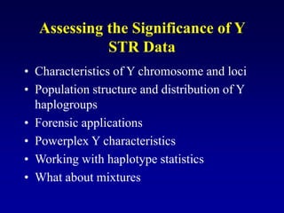
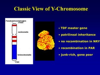
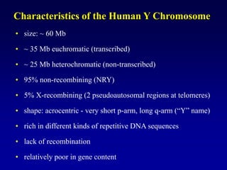
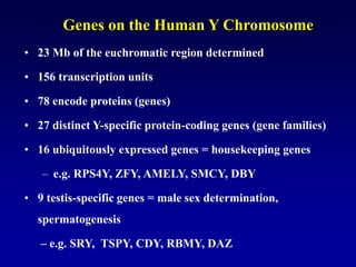
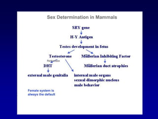
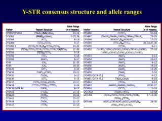
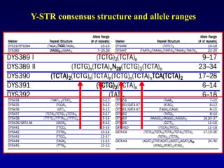
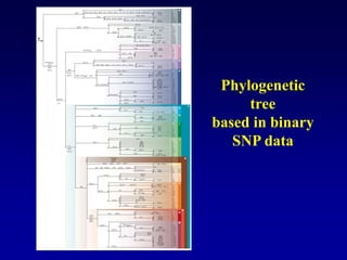
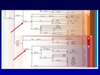
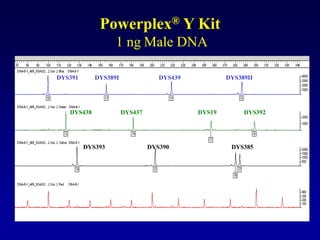
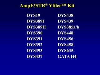
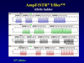
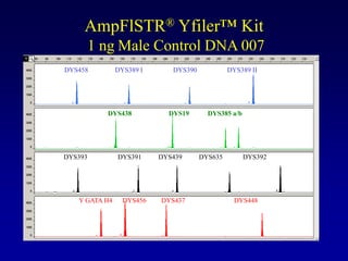
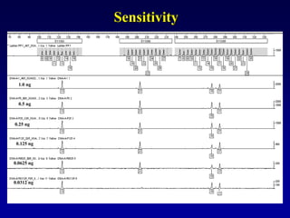
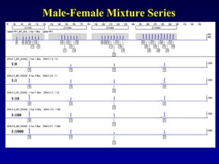
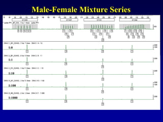
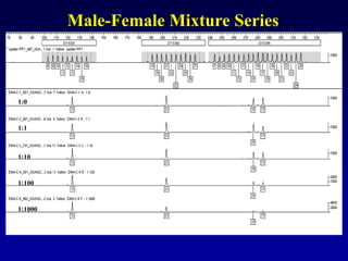
This document discusses applications of forensic genetics using Y-STR DNA analysis. It begins by describing characteristics of the human Y chromosome, including its size, gene content, and lack of recombination. It then discusses Y-STR polymorphisms and markers used in forensic kits. Examples are given of cases where Y-STR analysis was used, such as analyzing mixed male-female samples or determining paternity. Guidelines for interpretation and population studies using the PowerPlex Y kit are discussed. Common issues like sensitivity, mixtures, and anomalies are also summarized.

1. Applications in Forensic Genetics
John V. Planz, Ph.D.
UNT Center for Human Identification
Wisconsin Department of Justice
Madison, WI
January 4, 2008
Science and Statistics Behind
Y STR Systems

2. Assessing the Significance of Y
STR Data
• Characteristics of Y chromosome and loci
• Population structure and distribution of Y
haplogroups
• Forensic applications
• Powerplex Y characteristics
• Working with haplotype statistics
• What about mixtures

3. Classic View of Y-Chromosome
• TDF master gene
• patrilineal inheritance
• no recombination in NRY
• recombination in PAR
• junk-rich, gene poor

4. Characteristics of the Human Y Chromosome
• size: ~ 60 Mb
• ~ 35 Mb euchromatic (transcribed)
• ~ 25 Mb heterochromatic (non-transcribed)
• 95% non-recombining (NRY)
• 5% X-recombining (2 pseudoautosomal regions at telomeres)
• shape: acrocentric - very short p-arm, long q-arm (“Y” name)
• rich in different kinds of repetitive DNA sequences
• lack of recombination
• relatively poor in gene content

5. Genes on the Human Y Chromosome
• 23 Mb of the euchromatic region determined
• 156 transcription units
• 78 encode proteins (genes)
• 27 distinct Y-specific protein-coding genes (gene families)
• 16 ubiquitously expressed genes = housekeeping genes
– e.g. RPS4Y, ZFY, AMELY, SMCY, DBY
• 9 testis-specific genes = male sex determination,
spermatogenesis
– e.g. SRY, TSPY, CDY, RBMY, DAZ

7. Genes Mapped to Y Chromosome

8. Genes on the Human Y Chromosome
• 23 Mb of the euchromatic region determined
• 156 transcription units
• 78 encode proteins (genes)
• 27 distinct Y-specific protein-coding genes (gene families)
• 16 ubiquitously expressed genes = housekeeping genes
• 9 testis-specific genes = male sex determination, spermatogenesis
origin of NRY genes:
– derived / preserved from the proto-sex chromosomes
(X-homology)
– specialization in male-specific function

9. Evolution of Mammalian Sex Chromosomes
Lahn, Pearson & Jegalian 2001
Some homology with X – need to consider in validation

11. Polymorphisms of the Human Y Chromosome
Mutations create DNA polymorphisms and
these may serve as genetic markers
• Repetitive DNA – e.g., STRs
• Single-Copy DNA – e.g., SNPs, indels

12. Y Chromosome Polymorphisms
 ~ 200 binary polymorphisms (Y-SNPs) characterized
 > 300 microsatellites (Y-STRs) characterized
 1 minisatellite (MSY1)

13. Not all mutations
occur at the same
rate
‘hotspots’
‘coldspots’

14. Mutation Process for STR loci

15. Y-STR consensus structure and allele ranges

16. Y-STR consensus structure and allele ranges

17. Phylogenetic
tree
based in binary
SNP data

20. -From J.M. Butler (2003) Forensic Sci. Rev. 15:91-111
Forensic Y STR Systems

21. • Haplogroup: set of haplotypes defined
by slowly mutating markers (mainly
SNPs) which have more phylogenetic
stability.
• Haplotype: combination of allelic states
of a set of polymorphic markers lying on
the same DNA molecule.
Definitions
Unique event polymorphisms (UEP) record
history of Y chromosome

22. Why are our Y haplotypes so different?
• Many markers to choose from
• The selected loci are physically linked
• Markers have both SNPs and STRs
Infinite Sites Model
Stepwise Mutation
Model
Infinite Alleles Model

23. Population Differentiation
• Effective population size of Y chromosome is 1/4 of
autosomes or 1/3 of X
– lower sequence diversity on Y
– more susceptible to genetic drift
• random changes in frequency of haplotypes
due to sampling bias from one generation to
next
• accelerates differences between populations
• Variance of offspring further reduces Ne (effective
population size)

24. Population Differentiation
• Geographical clustering due to patrilocal behavior
of men
– women move closer to man’s birthplace
– local geographical differentiation enhanced
– Conquest effect
From Zerjal et al. Am. J. Hum. Genet. 72:717–721, 2003

25. Population Differentiation
• Geographical clustering due to patrilocal behavior
of men
– women move closer to man’s birthplace
– local geographical differentiation enhanced
– Conquest effect
You must consider that we are not talking
about contemporary populations when
discussing this!
Converse seen with mtDNA in Native American
Populations

26. Forensic Y-STR Applications
– Detect male DNA in a sample containing
male and female DNA (Huge background
of female DNA)
– Aspermic males
– Fingernail Scrapings
– Additional Power of Discrimination
– Multiple male donors
– Limits of differential extraction/ tissues
– Gender clarification (amelogenin)

27. Finger Nail Scraping Case
• Victim was found strangled to death
• Suspect had scratches on his face
• Based on STR results, suspect could not be
excluded; many alleles were below
interpretation threshold (inconclusive
result)
A Forensic Application

28. Evidentiary
Profile
Suspect
Profile

29. Identification of Male Contributor DNA in
Crime Scene Material
Autosomal STR profile
Female Victim DNA:
Male Suspect DNA:
Large Female DNA:
Perpetrator Male DNA
- See only female DNA profile
- Or partial DNA profile
- no female DNA
- no profile overlap
- only male component
Y STR profile

30. Investigations regarding Paternal Lineages
• Paternity Testing
• Kinship Analysis
• Deficiency cases
• Mass disasters
• Missing Persons
• Unidentified Remains

31. Deficiency Case Male Lineage
• Y STR analysis - any male relative in pedigree can be a
reference for alleged father
?

32. **Remember paternal lineage issues for identity testing

33. Y-STR Haplotype Analysis in Deficiency Paternity Case
DYS19 DYS389I DYS389II DYS390 DYS391 DYS392 DYS393 DYS385 DYS413 YCAII
Nephew 14 13 30(16) 25 11 13 12 11-14 22-22 3-7
Son 14 12 29 (16) 24 10 15 12 11-14 22-22 3-7
Exclusion
If true biological nephew, then alleged father is excluded as father of child in question
?
Kayser et al. Progress in Forensic Genetics (1998), 7: 494-496

34. • For effective use, guidelines are needed
• ISFG Recommendations
• Combine with existing recommendations (NRC II
Report)
• Nomenclature, Allelic Ladders, Population Genetics,
Statistical Issues

35. • Similar to autosomal STRs
• Thresholds for detection and interpretation
• Stutter
• Mixtures – what constitutes a mixture
• Validation studies in concert with guidelines
• Interpret evidence before knowns
Basic Interpretation Guidelines

37. Y STR LOCI
• DYS19
• DYS398 I
• DYS398 II
• DYS390
• DYS391
• DYS392
• DYS393
• DYS385 I/II
“Minimal Haplotype” – defined for research only

38. DYS19
DYS389I
DYS389II
DYS390
DYS391
DYS392
DYS393
DYS438
DYS439
DYS385a/b
Y STR Loci
SWGDAM
DYS385 – two loci
DYS389 – two loci

39. DYS385 a/b
a = b a  b
DYS389 I/II
I
II
F primer F primer
R primer
a b
Duplicated regions are 40,775
bp apart and facing away from
each other
F primer
R primer
F primer
R primer
DYS389I DYS389II
Figure 9.5, J.M. Butler (2005) Forensic DNA Typing, 2nd Edition © 2005 Elsevier Academic Press
Multi-Copy (Duplicated) Marker
Single Region but Two PCR
Products (because forward
primers bind twice)

40. • Commercially available Y-STR multiplex kits ---
allow for standard markers and QA/QC
• Most have EMH and SWGDAM recommended
loci
• Extra loci added to enhance discrimination
Kits

41. DYS19
DYS389I
DYS389II
DYS390
DYS391
DYS392
DYS393
DYS437
DYS438
DYS439
DYS385a/b
PowerPlex® Y System

42. Powerplex® Y
92 alleles
Allelic ladder

43. Powerplex® Y Kit
1 ng Male DNA
DYS391 DYS389I DYS439 DYS389II
DYS438 DYS437 DYS19 DYS392
DYS393 DYS390 DYS385

44. DYS19
DYS389I
DYS389II
DYS390
DYS391
DYS392
DYS393
DYS437
AmpFlSTR® Yfiler™ Kit
DYS438
DYS439
DYS385a/b
DYS448
DYS456
DYS458
DYS635
GATA H4

45. AmpFlSTR® Yfiler™
137 alleles
Allelic ladder

46. AmpFlSTR® Yfiler™ Kit
1 ng Male Control DNA 007
DYS458 DYS389 I DYS390 DYS389 II
DYS438 DYS19 DYS385 a/b
DYS393 DYS391 DYS439 DYS635 DYS392
Y GATA H4 DYS456 DYS437 DYS448

47. What can we expect?
Powerplex® Y
• Sensitivity
• Mixtures
• Anomalies

49. 0.0312 ng
1.0 ng
0.5 ng
0.25 ng
0.125 ng
0.0625 ng
Sensitivity

50. Sensitivity
0.0312 ng
1.0 ng
0.5 ng
0.25 ng
0.125 ng
0.0625 ng

51. Sensitivity
0.0312 ng
1.0 ng
0.5 ng
0.25 ng
0.125 ng
0.0625 ng

52. Male-Female Mixture Series
1:0
1:1
1:10
1:100
1:1000

53. Male-Female Mixture Series
1:0
1:1
1:10
1:100
1:1000

54. Male-Female Mixture Series
1:0
1:1
1:10
1:100
1:1000

55. Of course, with Male:Male mixtures you will get
more peaks at each locus.
Sensitivities down to about 5% minor contributor
are typical.
You cannot bank on peak height differences to
remain consistent across the dyes or loci, so be
careful when trying to physically deconvolute
these mixtures… this may not be a valid practice!
i.e. If target input DNA is 0.5 ng…
5% minor contributor is only 0.025 ng

56. These types of issues should raise some
operational questions:
 Input DNA:
• Total Genomic?
• Y specific?
• Increase to bring up minor?
• Impact of stutter?
Valid lab policies and interpretation
guidelines must be based on empirical data!

57. Stutter Issues
From Fulmer et al. 2007 Promega Application Notes

58. DYS389II
N-1, N-2 stutter is
commonly seen at all
input template
amounts.
1.0 ng
0.5 ng
0.25 ng

59. DYS392
N-1, N+1 stutter is
commonly seen at all
input template
amounts… this is
common among
trinucleotide repeat
loci.
1.0 ng
0.5 ng
0.25 ng

60. As with all typing systems, there are anomalies
that you should be aware of !
The majority of female samples will not
produce typing results with the Y STR kits…
But remember…the Y and X are functional
homologues and recombination IS possible.
 always run a female “victim” known
when using Y STR kits in the male –
female context!

61. Other observed Powerplex® Y anomalies
DYS19 Primer binding mutation
This was in an Asian (Hong Kong) Chinese sample

62. Other observed Powerplex® Y anomalies
DYS385
“Gene” duplication at DYS385
DYS385 a/b
a b
F primer
R primer
F primer
R primer
Multiple mutation steps
in the lineage are needed
to explain this one!!

63. Multiband Y Patterns
• MN ASIAN PA0077 DYS385 - 3 Bands
• MN HISPANIC PH0031 DYS390 - 2 Bands
• MN HISPANIC PH0063 Multibands
• NYC HISPANIC 26 DYS19 - 2 Bands
• NYC CAUCASIAN 4 DYS19 - 2 Bands
• CT HISPANIC 00-1851 DYS19 - 2 Bands
• CT HISPANIC 99-1695 DYS19 - 2 Bands
• CT HISPANIC 99-0362 DYS19 - 2 Bands
• CT HISPANIC 98-2136 DYS19 - 2 Bands
• CT CAUCASIAN 00-3022 DYS385 - 3 Bands
• ASIAN A-FTA-34-F/C DYS385 - 3 Bands
• ASIAN A-FTA-36-F/C DYS19 – Primer Binding site?
• ASIAN A-FTA-32-F/C DYS385 - 4 Bands
Must consider
this when
considering a
mixture

64. Population studies with Powerplex® Y
Before we can approach interpretive or
statistical understanding of the system we need
to understand what we are dealing with as a
locus…and yes, the whole set of markers in
Powerplex Y are just that…a single locus.
Several typical validation issues just don’t
matter with a Y haplotype system:
• Peak height ratio
• Hardy-Weinberg Equilibrium
But other things do!

65. CFS AFR
CT AFR
MI AFR
NYC AFR
TX AFR
CFS CAU
CT CAU
MI CAU
NYC CAU
TX CAU
CT HIS
Population
37
182
86
80
192
57
164
97
83
194
160
N
MI HIS
MN HIS
NYC HIS
TX HIS
Apache
Navajo
CFS ASN
MN ASN
NYC ASN
TX ASN
CFS EI
Population
97
101
80
192
138
219
28
101
45
73
37
N
Y STR Population Data
Promega Study
Total = 2443

66. DYS19
Allele Frequencies
African American
0
0.05
0.1
0.15
0.2
0.25
0.3
0.35
0.4
0.45
0.5
12 13 14 15 16 17 18
Alleles
Frequency
Sinha (n=543)
CFS (n=37)
CT (n=182)
MI (n=86)
NYC (n=80)
TX (n=193)

67. fi = frequency of each haplotype n = # haplotypes
h = n(1-fi
2)/ (n-1)
Haplotype Diversity
P =  fi
2
Haplotype Random Match Probability
Population Parameters

68. Haplotype Diversity
Hispanic
0
0.1
0.2
0.3
0.4
0.5
0.6
0.7
0.8
DYS437 DYS19 DYS392 DYS393 DYS390
CT HIS MI HIS MN HIS NYC HIS TX HIS

69. CFS AFR
CT AFR
MI AFR
NYC AFR
TX AFR
CFS CAU
CT CAU
MI CAU
NYC CAU
TX CAU
CT HIS
MI HIS
MN HIS
NYC HIS
TX HIS
Y Haplotype Profiles
Population
37
182
86
80
193
57
163
97
83
194
158
97
100
80
192
N # Haplotypes
36
172
85
80
181
50
153
87
80
170
130
90
95
74
179
% Single
97.3
94.5
98.8
100
93.8
87.7
93.9
89.7
96.4
87.6
82.3
92.8
95.0
92.5
93.2
Haplotype
Diversity
0.9985
0.9994
0.9997
>0.9999
0.9993
0.9944
0.9991
0.9968
0.9991
0.9981
0.9963
0.9985
0.9988
0.9968
0.9991

70. Apache
Navajo
CFS ASN
MN ASN
NYC ASN
TX ASN
CFS EI
Y Haplotype Profiles
138
219
28
100
45
70
37
70
101
28
96
43
69
35
50.7
46.1
100
96.0
95.6
98.6
94.6
0.9701
0.9806
>0.9999
0.9992
0.9970
0.9996
0.9955
Population N # Haplotypes % Single
Haplotype
Diversity

71. high haplotype diversity = high intra-individual variation
Haplotype Diversity
N>80
0.955
0.96
0.965
0.97
0.975
0.98
0.985
0.99
0.995
1
1.005

72. What about Linkage Equilibrium?
Intuitively, since these markers are all on a
single chromosome we’d predict strong
linkage and a lack of independence between
the loci.
Although this is very different from what
we are used to with our beloved CODIS
loci…this is what we expect with a
haplotype
What do we get?

73. CFS AFR
CT AFR
MI AFR
NYC AFR
TX AFR
CFS CAU
CT CAU
MI CAU
NYC CAU
TX CAU
CT HIS
MI HIS
MN HIS
NYC HIS
TX HIS
Population
37
182
86
80
193
57
163
97
83
194
158
97
100
80
192
N # Equilibrium
35
23
27
34
21
30
26
30
22
11
26
33
42
35
37
Y STR Loci Pairwise Tests
12 Loci – 66 tests

74. Apache
Navajo
CFS ASN
MN ASN
NYC ASN
TX ASN
CFS EI
Y STR Loci Pairwise Tests
12 Loci – 66 tests
Population
138
219
28
100
45
70
37
N
9
12
60
50
47
50
35
Fewest – Native American
Most – Asian (sample size; but Minnesota and Texas)
# Equilibrium

75. 391/389I
391/389II
389I/439
389I/385-2
439/389II
439/393
439/385-1
439/385-2
389II/393
437/393
Loci
19
18
17
18
17
19
18
20
17
18
# Populations
Y STR Loci Pairwise Tests
22 populations; ≥ 17 Equilibrium detected
What’s going on here??? – No detectable linkage?

76. 391/438
389I/389II
438/437
438/19
438/392
438/385-1
438/385-2
437/385-1
19/392
19/385-1
392/385-1
390/385-1
385-1/385-2
Loci
5
1
4
4
3
0
4
5
5
3
5
5
3
# Populations
Y STR Loci Pairwise Tests
22 populations; ≤ 5 Equilibrium
This is what we’d
expect…
Strong linkage

77. 389I/392
438/439
437/439
437/385-2
390/385-2
Loci
15
11
16
12
12
# Populations/
Equilibria
Y STR Loci Pairwise Tests
22 Populations – Examples of Population Specific Disequilibrium
Caucasian
Caucasian
Caucasian
African American
African American
Population/
Equilibria
Likely due to haplogroup differences among populations

78. • There is evidence of “independence” between
some of the loci in some of the populations
• A combination of mutation rate, subdivision
and random drift can cause this.
• One of the biggest factors is Haplogroup
Diversity
• The marker selection for increasing haplotype
diversity is not directly correlated to gene
diversity.
What do we see?

79. Approaching Analysis
• Some may suggest - “Use the set of Core Y STRs
and add more as needed to resolve matches”
• First question – when do you stop?
• If you get a match, you would have to continue on
ad infinitum!
• Is this a sensible policy?
How much power is needed???

80. Y-STR marker
combination
African
American
(N=786)
Caucasians
(N=778)
Hispanics
(N=381)
European minimal
haplotype (9) 75.8% 61.7% 79.8%
Eur. Minimal +
SWGDAM (11) 86.8% 74.3% 85.6%
PowerPlex® Y
(12) 87.7% 76.7% 88.2%
AmpFlSTR®
Yfiler kit
(17)
97.6% 95.5% 95.8%
Discriminatory Capacity* for three
U.S. populations
*DC= (# of different haplotypes / pop. size) x 100
Mulero et al., JFS (2006) 51:64-75

81. Number of Unique Haplotypes Observed for
Three U.S. Populations
Y-STR marker
combination
African
American
(N=786)
Caucasians
(N=778)
Hispanics
(N=381)
European
minimal
haplotype (9)
496 382 266
Eur. Minimal +
SWGDAM (11) 618 503 295
PowerPlex® Y
(12) 628 524 306
AmpFlSTR®
Yfiler kit
(17)
749 714 350
Mulero et al., JFS (2006) 51:64-75

82. Sample Info DYS19 DYS385 1
DYS389I 1
DYS389II 1
DYS390 1
DYS391 1
DYS392 1
DYS393 1
DYS438 1
DYS439 1
DYS437 1
DYS448 1
DYS456 1
DYS458 1
Y GATA H4 1
DYS635
C37 14 11,14 13 29 24 11 13 13 13 12 14 19 15 17 12 23
C330 14 11,14 13 29 24 11 13 13 13 11 15 19 15 19 11 23
ATCC 14 11,14 13 29 24 11 13 13 12 13 15 19 15 17 13 23
C304 14 11,14 13 29 24 11 13 13 12 13 15 19 17 18 12 23
C327 14 11,14 13 29 24 11 13 13 12 13 15 19 16 16 12 24
C63 14 11,14 13 29 24 11 13 13 12 13 15 17 16 17 11 23
C177 14 11,14 13 29 24 11 13 13 12 12 15 21 17 19 12 24
C198 14 11,14 13 29 24 11 13 13 12 12 15 18 16 17 12 23
C276RL 14 11,14 13 29 24 11 13 13 12 12 15 19 15 19 12 23
C294 14 11,14 13 29 24 11 13 13 12 12 15 19 15 17 11 24
C236 14 11,14 13 29 24 11 13 13 12 12 14 19 15 18 12 23
C85RL 14 11,14 13 29 24 11 13 13 12 12 14 19 16 16 11 24
C12 14 11,14 13 29 24 11 13 13 12 11 15 19 17 18 12 23
C194 14 11,14 13 29 24 11 13 13 12 11 15 19 17 17 12 23
C197 14 11,14 13 29 24 11 13 13 12 11 15 19 15 16 >13 24
C318 14 11,14 13 29 24 11 13 13 12 11 15 19 16 17 12 23
C345 14 11,14 13 29 24 11 13 13 12 11 15 19 15 18 12 23
C66RL 14 11,14 13 29 24 11 13 13 12 11 15 19 16 19 12 23
C205 14 11,14 13 29 24 11 13 13 12 11 14 19 15 17 12 23
C158 14 11,14 13 29 24 11 13 13 12 10 15 19 16 20 13 23
Common haplotype identified by the
European Minimal Haplotype markers
(20 individuals in Yfiler haplotype database*)
European Minimal
Haplotype
0
# of different
haplotypes 20
YfilerTM
8
PP Y
* http://www.appliedbiosystems.com/yfilerdatabase/

83. So…the logic does work…
More loci… better resolution…
But…doesn’t the size of the database matter?

84. European Minimal
Haplotype
0
# of different
haplotypes 20
YfilerTM
6
PP® Y
Individuals
sharing
haplotypes
20 4, 4, 2, 6 0
Point
Estimate
(N = 3561)
0.0056 0.00028
0.0011
0.0011
0.0006
0.0017
N= 1000 0.02
0.004
0.004
0.002
0.006
0.001

85. Approaching Analysis
• Unlikely approach because information gain is low
• Many samples will already be very limited
• Community will rely on commercially available kits
not in-house designer systems
• QC/ Proficiency Testing
• Better to increase size of database(s) to gain power
• We will re-visit substructure issues later

86. Approaching Analysis
• Some may suggest - “A reference database should
contain related individuals” – to better define the
population
• Probability of paternal relative having the same
haplotype is usually 1
• Databases are typically comprised of unrelated
individuals
• Although a small unknown number of related
individuals may be in a database
• Able to address significance of a very closely related
profile

87. Exclusion with 1 mismatch among 12 analyzed Y-
STRs
Evidence 14 12 28 25 11 11 13 14,14 11 11 15
Known 14 12 28 24 11 11 13 14,14 11 11 15
By having a database of unrelated males one can
assess weight of relative (with mutation) versus rarity
of haplotype in population

88. Qualitative Conclusions of Y-STR
Haplotype Comparison
Exclusion
- The two haplotypes are dissimilar; i.e, the
reference person is excluded as the contributor
of Y-specific DNA of the evidence sample
Inclusion/Match
- The Y haplotypes from two samples are
sufficiently similar and potentially could have
originated from the same source, or from a
common paternal lineage
Inconclusive
- Exclusion/Inclusion cannot be definitively
inferred due to insufficient data from one or
both of the DNA samples

89. Calculation to Convey to the Court
• Frequency estimate not possible
• Court desires a frequency estimate
• Point Estimate (Counting Method)
• Confidence Interval
• Approach the same as mtDNA

90. • The vast majority of possible haplotypes
will not be observed in any database
• The counting method is likely to be
conservative
• A correction for sampling
• A correction for substructure
Calculation to Convey to the Court
??

91. Calculation to Convey to the Court
Approaches
• It is more likely that the counting method will be
employed by the U.S. laboratories and courts
because of its operational simplicity

92. Limitations of the Counting Method
• Non-matched sites of the haplotype are given
weight equal to that of different origin (but
may have some extra value for substructure)
• Mutations are not weighted
• Haplotypes of the same paternal lineage can be
excluded, when they are subject to mutations
• Does not recognize evolutionary changes,
and/or effect of convergent mutations

93. CI = p ± 1.96 p(1-p)/N
For Y haplotype observed,
count the number of times
the profile is observed (X)
p = X/N
95% Upper bound on frequency
Where
• N is the size of the database

94. What about for Y haplotype that is not
observed in your database??
The upper bound of the CI is
1-1/N
Where
•  is the confidence level (0.05 for a 95% CI)
• N is the size of the database
Following: W. E. Ricker, 1937. Journal of the American Statistical Association, Vol. 32, No. 198: 349-356.

95. Maximum haplotype frequency
• If a Y-haplotype is not seen in a sample of N males
then at the  level of significance:
• Maximum frequency = 1 - 1/N
• Confidence level = 1- 
• As N becomes larger, maximum frequency becomes
closer to point estimate
This is why databases will drive our
statistical strength

96. N frequency
• 100 3/100 (0.03)
• 500 3/500 (0.006)
• 1,000 3/1,000 (0.003)
• 10,000 3/10,000 (0.0003)
Haplotype frequency

97. Calculation to Convey to the Court
Confidence Interval
• In many instances, the evidentiary haplotype may
not be observed in the reference database
• As a consequence, the usual assumption of a
Normal distribution may not apply for Y-STR
haplotype frequency estimates
• Ricker’s theory (1937) accommodates this
requirement
• The counts as well as the confidence bounds are
divided by the number of haplotypes sampled in the
entire database to estimate the probability of a
match

98. Online available Y-STR haplotype
reference databases
How de we actually get our Haplotype frequencies?
http://www.appliedbiosystems.com/yfilerdatabase/
Applied Biosystems Yfiler
http://www.promega.com/techserv/tools/pplexy/default.htm
Promega Powerplex Y

99. AB Yfiler

101. Haplotype data can be input manually or through
file upload.

102. Of Course,
There are no
matches
when testing
this many
loci.

105. A random Y haplotype

106. Haplotype data are input manually

107. Of Course,
There are no
matches
when testing
this many
loci.

108. So using our formula from before and an  = 0.05
1-1/N
1 – (0.05)1/4004 = 0.00075

111. So, lets try a haplotype that has been seen in
the Database…

112. A general search
returns 21 matches
in the database.

113. CI = p ± 1.96 p(1-p)/N
What p…?
What N…?

114. We can evaluate these
matches by looking at
the distribution of
matches among the
various population
groups.

117. CI = p ± 1.96 p(1-p)/N
We can do like we did before…looking at the
frequency in the whole database:
CI = 0.0052 + 1.96√ (0.0052(0.9948))/4004
Upper bound would be:
0.00743

118. CI = p ± 1.96 p(1-p)/N
Or we could do specific to the population group
in which the match was found:
CI = 0.0076 + 1.96√ (0.0076(0.9924))/1311
Upper bound would be:
0.0123
Caucasians

119. CI = p ± 1.96 p(1-p)/N
Or we could do specific to the population group
in which the match was found:
CI = 0.0067 + 1.96√ (0.0067(0.9933))/894
Upper bound would be:
0.01205
Hispanics

120. CI = p ± 1.96 p(1-p)/N
Or we could do specific to the population group
in which the match was found:
CI = 0.0036 + 1.96√ (0.0036(0.9964))/1108
Upper bound would be:
0.00712
African American

121. • Correction for population structure may be considered
• Effective population size ¼ of autosomal loci
• May actually be a little lower
• Substructure effects less in US than ancestral
populations
• Use when reference database considered not
representative
Calculation to Convey to the Court
Population Substructure

122. Problems created by population subdivision
Haplotype frequencies calculated
from population average
frequencies couldlead to:
–Wrong estimates!

123. Employ a Theta (q ) Correction
q is used as a measure of the effects of
population substructure
(inbreeding, coancestry)

124. NRCII q recommendation was pragmatically set
Empirical values are much less for autosomal
loci
National Academy of Sciences
May 1996

125. Still need to calculate substructure effects
But likely to be low for most major
populations, if evaluated under a
forensic model vs that of an
evolutionary model

126. U.S. Y-STR Haplotype Reference Database
www.ystr.org/usa
AA CAU HIS Total
Number of populations
sampled
10 11 9 30
Number of individuals
sampled
599 628 478 1,705
Number of Y-STR loci typed
(EMH)
9 9 9 9
Number of different
haplotypes
454
76%
437
70%
354
74%
1116
65%
Haplotype diversity 99.8% 99.6% 99.5% 99.7%
Most frequent haplotype 12
2.0%
25
3.98%
19
3.97%
53
3.1%
Kayser et al. J. Forensic Sci. (2002), 47(3): 5513-519

127. Hispanic
Structure of U.S. Populations with Y-STR Haplotypes
Florida EA
European-American
African-American
Virginia AA
Florida AA
Maryland AA
Texas AA
New York AA
Pennsylvania AA
Missouri AA
Oregon AA
Indiana AA
Lousiana AA
Pennsylvania EA
New York EA
Indiana EA
Missouri EA
Lousiana EA
Maryland EA
Pennsylvania H
Florida H
New York H
Connecticut H
Texas EA
Cajun EA
Virginia EA
Oregon EA
Oregon H
Maryland H
Lousiana H
Texas H
Virginia H
RST = 0.1
RST: measure for population differentiation
Kayser et al. J. Forensic Sci. (2002), 47(3): 5513-519

128. African American
Asian
Caucasian
Hispanic
Native American
Afr-Cau-His
All 5
Population
Partition (%) of genetic variance
(AMOVA)
98.96
98.69
98.45
99.08
96.98
87.19
83.40
A
A = within sample population
1.04
1.31
1.55
0.92
3.02
1.02
1.25
B
B= among sample populations within major population group (or regional variation)
---
---
---
---
---
11.79
15.35
C
C = among major population components for North American populations

129. FST
(AMOVA)
African American
Asian
Caucasian
Hispanic
Native American
Afr-Cau-His
All 5
Population
0.0104
0.0131
0.0155
0.0092
0.0302
0.1179
0.1535
FST
AMOVA routine (with the option of allele size difference) of Arlequin 2.0
ST

130. FST
(AMOVA)
African American
Asian
Caucasian
Hispanic
Native American
Afr-Cau-His
All 5
Population
0.0051
0.0148
0.0071
0.0061
0.0188
0.0745
0.1001
FST
Note: Asian is likely inflated and more data are needed to assess FST
0.0104
0.0131
0.0155
0.0092
0.0302
0.1179
0.1535
ФST
AMOVA routine (without the option of allele size difference) of Arlequin 2.0

131. FST
(AMOVA)
African American
Asian
Caucasian
Hispanic
Native American
Afr-Cau-His
All 5
Population
0.0051
0.0148
0.0071
0.0061
0.0188
0.0745
0.1001
FST
0.0006
0.0039
-0.0005
0.0021
0.0282
------
------
FST
autosomal

132. f (haplotype) = pi + q (1- pi)
Formula
Note: θ is the limiting factor!
With q of 0.01 and our p of 0.00028:
0.00028 + (0.01 x (1 – 0.00028))
0.00028 + 0.0099
≈ 0.0103

133. q
Pool populations ---
Impact
• US populations
• Intra-individual variation
• Most common haplotypes the same
• What is the frequency of unknown or uncommon
haplotypes in different datasets?
• Even if there is substructure
Most frequent

134. Y STR haplotype is one locus with many alleles
A1
A2
.
.
.
.
A100
Population 1
A101
A102
.
.
.
.
A200
Population 2
Databases with reasonable size
approximate this model
θ is almost 0

135. A1
A2
.
.
.
.
An
Population 1
A1'
A2'
.
.
.
.
An'
Population 2
In reality, with large number of loci a few types are shared
and most if not all have never been seen in the database
θ approaches 0
Y STR haplotype is one locus with many alleles

136. So the more loci typed,
the more haplotypes/alleles will be in the database
Thus, multi-locus kits are valuable for this aspect
q approaches 0
In the process of calculating q under forensic model***
Y STR haplotype is one locus with many alleles

137. Forensic Model
Population Substructure
DYS19 DYS389I DYS389II DYS390 DYS391 DYS392 DYS393 DYS385
A --- 14 12 29 24 10 15 12 11-14
E --- 18 12 25 24 10 15 15 11-18
B --- 14 13 29 24 10 15 12 11-14
C --- 14 13 29 24 12 15 12 10-14
D --- 18 11 25 24 10 13 15 12-18
Which haplotypes might be more closely related?

138. Forensic Model
Population Substructure
DYS19 DYS389I DYS389II DYS390 DYS391 DYS392 DYS393 DYS385
A --- 14 12 29 24 10 15 12 11-14
C --- 14 13 29 24 12 15 12 10-14
Are such evolutionary differences
considered in forensic evaluation?
E --- 18 12 25 24 10 15 15 11-18
A --- 14 12 29 24 10 15 12 11-14
Exclusion
Exclusion

139. Locus Caucasian
(N = 199)
Afr Amer
(N = 203)
Hispanic
(N = 207)
Asian
(N = 83)
Total
(N = 692)
DYS391 11:10 1
DYS389I 12:13 1
DYS389II 29:30 30:29 1*
DYS439 13:12 11:12 2
DYS438 0
DYS437 15:16 15:14 2
DYS19 16:17 2
17:16
DYS392 0
DYS393 14:15 1
DYS390 0
DYS385 14:15 14:15 12,14:14 3
Total 2/2388 6/2436 2/2484 3/996 13/8304
0.00084 0.00246 0.00081 0.0031 0.00157
Y STR mutations (father:son allele transmission)

140. • 692 confirmed father-son pairs (probability > 99.9%)
• 14 mutation events were observed
• Average rate of 1.57 x 10-3/locus /generation (13/8304)
• With a 95% confidence bound of 0.83 x 10-3 to 2.69 x 10-3
• This rate is a little smaller than that of the Kayser, et al.
• Estimate (2.80 x 10-3/locus)
• But the difference is not statistically significant (P > 0.05).
one Asian father-son pair at the DYS389I/II loci complex (12,29)  (13, 30)
appears as a double mutation, but likely is a single original event.
Y STR mutations (father:son allele transmission)

141. Mutation??
Likelihood calculation
14, 12, 28, 22, 10, 11, 14, 13-14, 19-21
14
14, 12, 28, 22, 10, 11, 13, 13-14, 19-21
13
Mutation: µ (DYS393) = 3.2 x 10-3
?
f obs= 0.001
fobs = 0.007
7
5
Paternal Relatives share the same haplotype
Are they related?
L(X) = 0.001 x 5 x µ/2 + 0.007 x 7 x µ/2 (related)
L(Y) = 0.001 x 0.007 (non-related)
LR (X/Y) ≈ 12 for patrilinear relationship

142. Next Task
• Test independence between
autosomal loci and Y haplotypes

143. Independence Testing of Y Haplotype
and 13 Autosomal CODIS STR Loci
(Autosomal Locus/ Y Haplotype Displaying Disequilibria* - 22 populations)
1. Apache
FGA, p-value = 0.03760000
D21S11, p-value = 0.03460000
D18S51, p-value = 0.02820000
D5S818, p-value = 0.02660000
2. Minnesota Asian
D8S1179, p < 10-3
3. Minnesota Hispanic
D16S539, p-value = 0.03340000
D18S51, p-value = 0.02100000
4. Canada African American
FGA, p-value = 0.00920000
5. Canada Asian Indian
D7S820, p-value = 0.02820000
6. Connecticut African American
FGA, p-value = 0.04300000
THO1, p-value = 0.00280000
7. Connecticut Caucasian
THO1, p-value = 0.02880000
8. Michigan Caucasian
D16S539, p-value = 0.04820000

144. 13. New York Caucasian
D7S820, p-value = 0.01660000
14. New York Hispanic
D21S11, p-value = 0.01340000
15. Texas African American
D13S317, p-value = 0.01200000
D18S51, p-value = 0.01420000
16. Texas Hispanic
D5S818, p-value = 0.01880000
9. Michigan Hispanic
vWA, p-value = 0.03160000
FGA, p-value = 0.02240000
10. Native American Total
D3S1358, p-value = 0.02680000
D21S11, p-value = 0.00060000
D18S51, p-value = 0.00840000
11. Navajo
D21S11, p-value = 0.02820000
12. New York Asian
D16S539, p-value = 0.00740000
Independence Testing of Y Haplotype
and 13 Autosomal CODIS STR Loci
(Autosomal Locus/ Y Haplotype Displaying Disequilibria* - 22 populations)

145. Next Task
• Mixtures
• Assume 2 alleles for 11 loci
• 211 possible haplotypes with PP Y – 2048
• Most haplotypes not observed in database
• Assumption of independence not correct
• Minimal haplotype frequency (minimum
allele frequency) not practical

146. Mixture
• Probability of Exclusion
• Binomial distribution - haplotypes excluded and
haplotypes not excluded
• Count number (m) not excluded; (PI = m/n)
• Estimate upper CI of PI
• PE = 1- PI
• Based on same principles used for autosomal loci (but
at haplotype level)

147. • Four scenarios for two contributor sample in example:
•Hp --- S1 and S2 are source
• Hd --- S1 and unknown are source (same as PI)
• Hd --- S2 and unknown are source (same as PI)
• Hd --- two unknowns are source
Mixture
Likelihood Ratio

148. • Assume three loci, two alleles at each locus, two
male suspects
•Total alleles the same as in evidence
• Equal contribution
• 8 possible haplotypes
Mixture
Likelihood Ratio

149. 13/15 8/10 22/25 --- 3 locus profile
15 8 22 --- haplotype 2
15 8 25 --- haplotype 4
13 10 22 --- haplotype 5
15 10 22 --- haplotype 6
13 10 25 --- haplotype 7
13 8 25 --- haplotype 3
15 10 25 --- haplotype 8
13 8 22 --- haplotype 1
All haplotypes included are
PE/PI

150. PE/PI
All possible haplotypes are included
13/15, 8/10, 22/25 --- 3 locus profile
15 8 22 --- haplotype 2
15 8 25 --- haplotype 4
13 10 22 --- haplotype 5
15 10 22 --- haplotype 6
13 10 25 --- haplotype 7
13 8 25 --- haplotype 3
15 10 25 --- haplotype 8
13 8 22 --- haplotype 1
But certain haplotype pairs can not explain evidence
haplotype 1 + haplotype 2
haplotype 1 + haplotype 3
haplotype 1 + haplotype 4
haplotype 1 + haplotype 5
and so on

151. haplotype 1 + haplotype 8
haplotype 2 + haplotype 7
haplotype 3 + haplotype 6
haplotype 4 + haplotype 5
Only certain haplotype pairs can explain evidence
PE/PI
All possible haplotypes are included
13/15, 8/10, 22/25 --- 3 locus profile
15 8 22 --- haplotype 2
15 8 25 --- haplotype 4
13 10 22 --- haplotype 5
15 10 22 --- haplotype 6
13 10 25 --- haplotype 7
13 8 25 --- haplotype 3
15 10 25 --- haplotype 8
13 8 22 --- haplotype 1

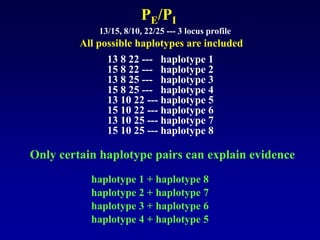
152. LR =
1
2[Pr(H1)Pr(H8) + Pr(H2)Pr(H7) + Pr(H3)Pr(H6) + Pr(H4)Pr(H5)]
Mixture
Likelihood Ratio

153. • Technically correct
• Can not estimate individual haplotype frequencies
• 217 (131,072) possible haplotypes (Yfiler)
211 (2048) possible haplotypes (PP Y)
• Not all combinations can explain the evidence
• Assuming independence is not correct
• Cannot place types in database, most never seen, too
many
Mixture
LR

154. Use same logic as PI
for the denominator in the LR
Haplotypes fall into either category
Only E/E can explain the evidence
and only a subset of these fit
E/E and E/E pairs can not explain the evidence
E = excluded E = not excluded

155. m*/n(n-1) and take upper CI as denominator
Mixture
LR
m* - those pairs (of E/E) that explain evidence

156. LR =
1
m*/n(n-1)
Mixture
LR
• The denominator is the PI with an assumed
number of contributors
• Makes better use of data

157. Online available Y-STR haplotype
reference databases
We still have the problem that none of these
(or PopStats) is designed to enable mixture
calculations!!
Calculation of reporting statistics is quite
straight-forward with the help of the searchable
databases
And doing this with 12 or 17 loci by hand…
…would be a bear!

158. John V. Planz, Ph.D
UNT Center for Human Identification
jplanz@hsc.unt.edu