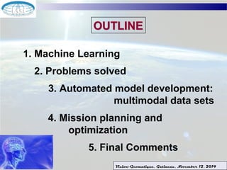
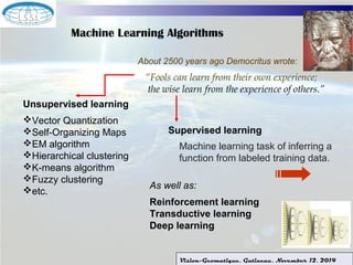
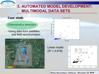
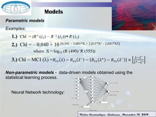
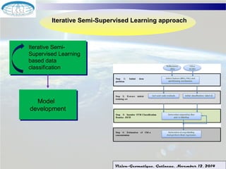
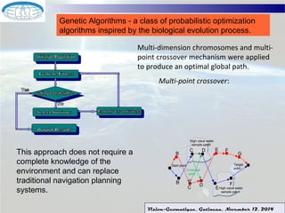
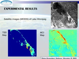
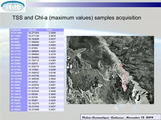
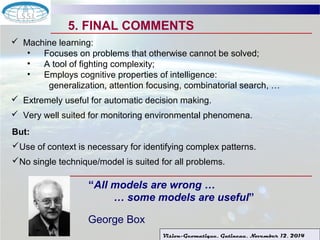
MACHINE LEARNING FOR SATELLITE-GUIDED WATER QUALITY MONITORING

1. MACHINE LEARNING FOR
SATELLITE-GUIDED WATER
QUALITY MONITORING
Marek B. Zaremba
Laboratoire de Systèmes Spatiaux Intelligents (LSSI)
Département d’informatique et d’ingénierie
Université du Québec en Outaouais
Gatineau, Canada
Vision-Geomatique, Gatineau, November 12, 2014

2. OOUUTTLLIINNEE
1. Machine Learning
2. Problems solved
3. Automated model development:
multimodal data sets
4. Mission planning and
optimization
5. Final Comments
Vision-Geomatique, Gatineau, November 12, 2014

3. 1. MACHINE LEARNING
Machine learning is a sub-field of artificial intelligence that is
concerned with the design and development of algorithms that
allow computers to learn the behavior of data sets empirically.
Vision-Geomatique, Gatineau, November 12, 2014
What is Machine Learning?
A major focus of machine-learning research is to
produce (induce) empirical models from data automatically.
WHY?
This approach is usually used because of the
absence of adequate and complete theoretical
models.
Can’t you do
anything
right?

4. Machine Learning Algorithms
About 2500 years ago Democritus wrote:
“Fools can learn from their own experience;
the wise learn from the experience of others.”
Machine learning task of inferring a
function from labeled training data.
Vision-Geomatique, Gatineau, November 12, 2014
Unsupervised learning
Vector Quantization
Self-Organizing Maps
EM algorithm
Hierarchical clustering
K-means algorithm
Fuzzy clustering
etc.
Supervised learning
As well as:
Reinforcement learning
Transductive learning
Deep learning

5. Supervised learning
Neural Networks
They learn complex nonlinear input-output
Backpropagation
Autoencoders
Hopfield networks
Boltzmann machines
Restricted Boltzmann Machines
Spiking neural networks
etc.
Support Vector Machines
relationships and adapt
themselves to the data, using
sequential training procedures.
SVMs map the training data into a
higher-dimensional feature space
via kernel mapping, and construct
a separating hyperplane with a
maximum error margin.
Vision-Geomatique, Gatineau, November 12, 2014
Linear classifiers
Fisher's linear discriminant
Logistic regression
Multinomial logistic regression
Naive Bayes classifier
Perceptron

6. 2. PROBLEMS SOLVED
Learning Algorithms – which are the best?
The No Free Lunch (NFL) theorem (Wolpert and Macready, 1995) has
shown that learning algorithms cannot be universally good. Matching
algorithms to problems gives higher average performance than does
applying a fixed algorithm to all.
Hence:
Experience with a broad range of techniques is the best
insurance for solving arbitrary new problems
General classes of problems:
Vision-Geomatique, Gatineau, November 12, 2014
 Classification
 Regression
 Optimization

7. Vision-Geomatique, Gatineau, November 12, 2014
Classification
problems
Supervised and unsupervised
Ex. Water/Land cover
classification

8. Regression problems
The use of machine learning can actually help us to construct
multivariate, nonlinear mappings between satellite radiances and the
suite of water products.
Vision-Geomatique, Gatineau, November 12, 2014
Example:
Non-parametric
inverse modeling
architectures:
-Allow us to obtain
complex bi-directional
radiative transfer models;
-Production very fast;
-Can be adapted to
different bio-optical
models and applied in
form of a NN library.

9. Optimization problems
If we start our search here
Vision-Geomatique, Gatineau, November 12, 2014
A local method will only find
local extrema
Using ML techniques:

10. 3. AUTOMATED MODEL DEVELOPMENT:
MULTIMODAL DATA SETS
140
120
100
80
60
40
20
0
Chlorophyll-a Distribution
-1 0 1 2 3 4 5 6
Chlorophyll-a concentration mg/m 3
MCI-MERIS
Vision-Geomatique, Gatineau, November 12, 2014
Case study
Chlorophyll-a detection
-Using data from satellites
and field spectrometers
Linear model
(R2 = 0.679):

11. Parametric models
Examples:
Models
Non-parametric models - data-driven models obtained using the
statistical learning process.
Neural Network technology:
Vision-Geomatique, Gatineau, November 12, 2014

12. The problem …
Biased (statistics systematically different from the population parameter) and
non-ergodic (distribution parameters vary in time) data sets
Biases are ubiquitous. With fusion of multiple datasets bias is often
an issue (very relevant for climate variables). Yet, we typically need
to fuse multiple datasets to construct long-term time series and/or
improve global coverage.
If the biases are not corrected before data fusion we introduce
further problems, such as spurious trends, leading to the
possibility of unsuitable policy decisions.
So what can we do about this?
.... we do not have a theoretical explanation (The Earth system is so
complex, with many interacting processes, and often the instruments are also
complex, this is not always possible to theoretically understand the
cause of the bias and data issues from first principles).

13. Iterative Semi-Supervised Learning approach
Vision-Geomatique, Gatineau, November 12, 2014
Iterative Semi-
Supervised Learning
based data
classification
Model
development
Model
development

14. Model development -
NN models
Before and after the Iterative
Semi-Supervised Learning
procedure:

15. 4. MISSION PLANNING AND OPTIMIZATION
Objective:
Optimization of the in-situ data acquisition process through the planning
of an optimal ship trajectory.
 The path planning system generates an optimal path with the goal of
maximizing the number and the value of the collected samples during
the acquisition mission.
 The acquisition mission can be varied depending on the strategy applied
to collect the samples for different water pollutants (Chl-a, TSS, DOC,
…) :
 Maximum gradient following strategy
 Maximum concentration areas
 Uniform coverage strategy
 Any strategy can be represented by an objective function.
æ
å NJ
= +å +å
C V /
N t D
i J  The strategies can be applied depending on the surrounding
environment and the data acquisition mission constraints.
ö
÷ ÷ø
ç çè
= = =
i
K
S
K
J
S
J
1 1 1

16. Broader context of Hybrid Intelligent Control
ψ
Mapping and
environment
modeling
α
Planning
P
E
Context
Reactive
Control
E
ΨE
π
Logic
Statement
Cost function
Deliberative
level
Reactive level
ΨR
The deliberative level control
architecture formally defined as:
DC ={E,y ,p ,P,a}
The reactive level deals with
the obstacles and the ship
maneuverability
Vision-Geomatique, Gatineau, November 12, 2014

17. Genetic Algorithms approach
Classes of Search Techniques:
GAs use different:
 Representations (chromosomes)
 Mutation and Crossover mechanisms
 Fitness functions
Vision-Geomatique, Gatineau, November 12, 2014

18. Genetic Algorithms - a class of probabilistic optimization
algorithms inspired by the biological evolution process.
Multi-dimension chromosomes and multi-point
crossover mechanism were applied
to produce an optimal global path.
Multi-point crossover:
High value water
sample patch
B C D E
Start point
D E
G
Target
point
F
High value water
sample patch
B
C
F
Crossover
point
This approach does not require a
complete knowledge of the
environment and can replace
traditional navigation planning
systems.
Vision-Geomatique, Gatineau, November 12, 2014

19. EXPERIMENTAL RESULTS
Satellite images (MODIS) of Lake Winnipeg
TSS
Map
MCI
Map
Vision-Geomatique, Gatineau, November 12, 2014

20. TSS and Chl-a (maximum values) samples acquisition
longitude latitude Value
-97.071594 52.271004 0.3949
-97.15443 52.271156 0.3678
-97.0877 52.163826 0.4037
-96.9688 51.998085 0.4001
-96.94884 51.884686 0.4083
-97.10551 51.87565 0.4532
-97.17112 51.886684 0.4526
-97.17112 51.886684 0.4378
-97.19144 51.804962 0.4324
-97.25087 51.705112 0.4360
-97.27605 51.62972 0.4971
-97.27722 51.555775 0.6226
-97.27228 51.47804 0.6288
-97.258446 51.456432 0.6196
-97.213425 51.470726 0.6044
-97.187546 51.485546 0.5692
-97.18434 51.53722 0.5521
-97.22941 51.522934 0.5597
-97.19398 51.577347 0.3957
-97.13055 51.624245 0.5948
-97.10014 51.69328 0.3663
-97.040436 51.83706 0.4298
-97.08387 51.95991 0.4200
-97.13075 52.102375 0.3001
-97.14458 52.231052 0.4037
-97.08629 52.273468 0.3931
Vision-Geomatique, Gatineau, November 12, 2014

21. 5. FINAL COMMENTS
Vision-Geomatique, Gatineau, November 12, 2014
 Machine learning:
• Focuses on problems that otherwise cannot be solved;
• A tool of fighting complexity;
• Employs cognitive properties of intelligence:
generalization, attention focusing, combinatorial search, …
 Extremely useful for automatic decision making.
 Very well suited for monitoring environmental phenomena.
But:
Use of context is necessary for identifying complex patterns.
No single technique/model is suited for all problems.
“All models are wrong …
… some models are useful”
George Box

22. Vision-Geomatique, Gatineau, November 12, 2014