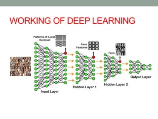
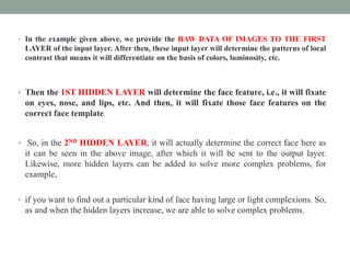
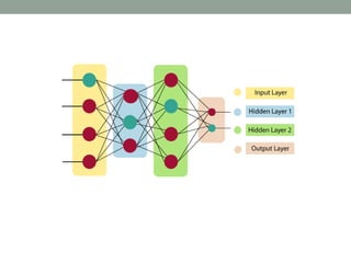
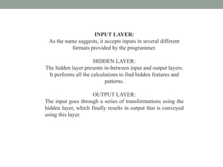
DEEP LEARNING
DEFINATION OF DEEP
LEARNING
WORKING OF DEEP LEARNING
• In the example given above, we provide the RAW DATA OF IMAGES TO THE FIRST
LAYER of the input layer. After then, these input layer will determine the patterns of local
contrast that means it will differentiate on the basis of colors, luminosity, etc.
• Then the 1ST HIDDEN LAYER will determine the face feature, i.e., it will fixate
on eyes, nose, and lips, etc. And then, it will fixate those face features on the
correct face template.
• So, in the 2ND HIDDEN LAYER, it will actually determine the correct face here as
it can be seen in the above image, after which it will be sent to the output layer.
Likewise, more hidden layers can be added to solve more complex problems, for
example,
• if you want to find out a particular kind of face having large or light complexions. So,
as and when the hidden layers increase, we are able to solve complex problems.
APPLICATIONS OF DEEP LEARNING
AMAZON ALEXA
• ADVANTAGES OF DEEP LEARNING
• 1. AUTOMATIC FEATURE LEARNING
• The algorithms employed in Deep learning are powered to automatically learn
features eliminating the need for hand-engineered intervention. This is especially
beneficial for tasks with difficult-to-define properties, such as picture recognition.
• 2. HANDLING HUGE AND COMPLICATED DATASETS
• Deep learning algorithms come with the potential of handling enormous and
complex datasets that typical traditional machine learning algorithms would
struggle to comprehend. This feature makes it a powerful tool that can be
leveraged in gaining insights from the colossal amount of data and huge datasets.
This is one of the most critical advantages of deep learning in comparison to other
traditional methods.
• 3. ENHANCED PERFORMANCE
• Deep learning algorithms have proven to generate a more cutting-edge
performance with their integration into an array of applications like image and
audio recognition, natural language processing, and computer vision.
• 5. HANDLING VARIED TYPES OF DATA
• Deep Learning algorithms have the capacity of handling structures as
well as unstructured data like Images, texts, and audio.
• 6. INCREASED CAPACITY GIVEN THEIR COMPLEXITY
• This is yet another notable advantage of deep learning. Machine learning
types like Deep learning that employs neural networks with multiple
hidden layers are highly suitable for large-scale and high-dimensional
problems. This is prompted by its large number of parameters. It can
simulate intricate or complex non-linear correlations in data making it
highly suitable for complex data sets.
• 7. UNSUPERVISED AND AUTOMATED LEARNING
• Deep learning also boasts the advantage of being trainable to learn data
representations and either perform tasks or initialize supervised learning
models using unsupervised representation learning. It can also provide
valuable and important features or skills without the need for human
intervention.
• 8. ADAPTABILITY AND SCALABILITY
• Deep learning models are highly adaptable. The models can be
fine-tuned or adapted to new tasks with a limited amount of
labeled data by employing and leveraging information acquired
from previous tasks. This top advantage of Deep learning
comes in handy in application or use-case requirements where
there is a dearth of labeled data.
• 9. ABILITY TO HANDLE LACKING OR MISSING DATA
• Another advantage of deep learning is its capacity to function
even when data is lacking. A specific model can handle missing
or absent data by learning to automatically impute missing
values. This makes it an appropriate and ideal tool for
scenarios involving incomplete or distorted data.
• DISADVANTAGES OF DEEP LEARNING
• 1. REQUIRES A LARGE AMOUNT OF DATA
• Deep Learning's advantage of using massive data as its training
dataset can cause a big advantage. A significant amount of High-
quality data is required for the proper functioning of a deep learning
model. This massive requirement demands a significant amount of
time as well as resources for obtaining data
.
• 2. EXTENSIVE COMPUTING NEEDS
• This is one of the major disadvantages of Deep learning. For training
a specific model with huge datasets necessitates more computing
resources than other machine learning models. Some of the
examples are -Powerful central processors and graphics processing
units, large amounts of storage and random access memories, etc.
• 3. OVERFITTING TENDENCIES
• One of the biggest disadvantages of Deep learning is its
problem of Overfitting. In the case of Overfitting, the model
performs well on training data but comparably poor on unseen
data. This may result in the model rendering irrelevant or
incorrect answers. This further results in undermining
automatic and transfer learning.
• 4. ISSUES WITH INTERPRETATION
• Another significant limitation of deep learning is that its models
can be complicated to interpret or explain, unlike the case with
traditional machine learning algorithms and models. Some
people may struggle to comprehend the operating mechanism
of the model or its decision-making processes.
RESULT ANALYSIS
INTRODUCTIONTONEURALNETWORK
• Neural Networks are computational models that mimic the complex functions of the human brain.
• The neural networks consist of interconnected nodes or neurons that process and learn from data, enabling
tasks such as pattern recognition and decision making in machine learning.
•
The given figure illustrates the typical diagram of
Biological Neural Network
The typical Artificial Neural Network looks something like the given
figure.
THE ARCHITECTURE OF AN
ARTIFICIAL NEURAL NETWORK
• IN ORDER TO DEFINE A NEURAL NETWORK THAT CONSISTS OF
A LARGE NUMBER OF ARTIFICIAL NEURONS, WHICH ARE
TERMED UNITS ARRANGED IN A SEQUENCE OF LAYERS. LETS US
LOOK AT VARIOUS TYPES OF LAYERS AVAILABLE IN AN
ARTIFICIAL NEURAL NETWORK.
• IN ORDER TO DEFINE A NEURAL NETWORK THAT
CONSISTS OF A LARGE NUMBER OF ARTIFICIAL
NEURONS, WHICH ARE TERMED UNITS ARRANGED IN
A SEQUENCE OF LAYERS.
INPUT LAYER:
As the name suggests, it accepts inputs in several different
formats provided by the programmer.
HIDDEN LAYER:
The hidden layer presents in-between input and output layers.
It performs all the calculations to find hidden features and
patterns.
OUTPUT LAYER:
The input goes through a series of transformations using the
hidden layer, which finally results in output that is conveyed
using this layer.
ADVANTAGES OF ARTIFICIAL NEURAL
NETWORK (ANN)
1. PARALLEL PROCESSING CAPABILITY:
Artificial neural networks have a numerical value that
can perform more than one task simultaneously.
2.STORING DATA ON THE ENTIRE NETWORK:
data that is used in traditional programming is stored on
the whole network, not on a database. the disappearance
of a couple of pieces of data in one place doesn't prevent
the network from working.
HARDWARE DEPENDENCE:
Artificial neural networks need processors with parallel
processing power, as per their structure. Therefore, the realization
of the equipment is dependent.
DIFFICULTY OF SHOWING THE ISSUE TO THE
NETWORK:
ANNs can work with numerical data. Problems must be
converted into numerical values before being introduced to ANN.
The presentation mechanism to be resolved here will directly
impact the performance of the network. It relies on the user's
abilities.
THE DURATION OF THE NETWORK IS UNKNOWN:
The network is reduced to a specific value of the error, and this
value does not give us optimum results.
DISADVANTAGES
APPLICATIONS OF ARTIFICIAL NEURAL NETWORKS
Social Media:
Marketing and Sales:
Frank Rosenblatt
• An MLP is a type of feed forward artificial neural network with multiple layers, including an input
layer, one or more hidden layers, and an output layer. Each layer is fully connected to the next.
• Multilayer Perceptron Neural Network is a Neural Network with multiple layers, and all its layers
are connected.
• It uses a Back Propagation algorithm for training the model. Multilayer Perceptron is a class
of Deep Learning, also known as MLP.
MULTILAYER PERCEPTRON
• Frank Rosenblatt first defined the word Perceptron in his perceptron
program.
• Perceptron is a basic unit of an artificial neural network that defines
the artificial neuron in the neural network.
• It is a supervised learning algorithm containing nodes’ values,
activation functions, inputs, and weights to calculate the output.
• The Multilayer Perceptron (MLP) Neural Network
works only in the FORWARD DIRECTION.
• All nodes are fully connected to the network. Each
node passes its value to the coming node only in the
forward direction.
• The MLP neural network uses a Back propagation
algorithm to increase the accuracy of the training
model.
• A multilayer perceptron (MLP) Neural network
belongs to the feed forward neural network.
• It is an Artificial Neural Network in which all nodes
are interconnected with nodes of different layers.
ADVANTAGES OF MULTILAYER PERCEPTRON
NEURAL NETWORK
• It can handle complex problems while dealing with large
datasets.
• Developers use this model to deal with the fitness problem
of Neural Networks.
• It has a higher accuracy rate and reduces prediction error
by using backpropagation.
• After training the model, the Multilayer Perceptron Neural
Network quickly predicts the output.
DISADVANTAGES OF MULTILAYER PERCEPTRON
NEURAL NETWORK
• This Neural Network consists of large computation, which
sometimes increases the overall cost of the model.
• The model will perform well only when it is trained
perfectly.
• Due to this model’s tight connections, the number of
parameters and node redundancy increases.
FORWARD PROPAGATION
• the input data is fed in the forward direction through the
network.
• Each hidden layer accepts the input data, processes it as
per the activation function and passes to the successive
layer.
WHY FEED-FORWARD NETWORK?
• In order to generate some output, the input data should be
fed in the forward direction only.
• The data should not flow in reverse direction during
output generation otherwise it would form a cycle and the
output could never be generated. Such network
configurations are known as feed-forward network.
• The feed-forward network helps in forward propagation.
ADVANTAGES:
Efficiency: Forward propagation is computationally efficient,
especially when compared to backpropagation, which involves the
calculation of gradients and requires more computational resources.
Parallelization: Since forward propagation involves independent
calculations for each neuron in a layer, it is highly amenable to
parallelization. This makes it well-suited for implementation on
parallel computing architectures like GPUs and TPUs, leading to faster
training times.
Real-time Prediction: Once a neural network is trained, forward
propagation can be used for real-time prediction or inference tasks.
This is because the process only involves passing the input data
through the network without any backward pass or weight updates.
Simplicity: The concept of forward propagation is relatively simple to
understand and implement, making it a foundational component of
neural network training algorithms.
.
DISADVANTAGES:
Limited to Feed forward Networks:
Forward propagation is primarily used in feedforward neural
networks, where information flows in one direction, from the
input layer to the output layer. It may not be directly
applicable to other types of neural networks, such as
recurrent neural networks (RNNs), which involve feedback
loops.
Initialization Dependency: The effectiveness of
forward propagation heavily depends on the initialization of
the network's weights and biases. Poor initialization can lead
to issues like vanishing or exploding gradients, which can
hinder training convergence
OPTIMIZATION TECHNIQUES IN DEEP LEARNING
* ROLE *
It plays a crucial role in deep learning and is essential for training neural networks effectively. Here are some key
aspects of optimization in deep learning:
• Model Training:
• Optimization algorithms are used to train deep learning models by adjusting the model's parameters to
minimize a loss function.
• The goal is to find the optimal set of parameters that best fit the training data and generalize well to unseen
data.
• Loss Function Optimization:
• Deep learning models are trained using a loss function that measures the difference between the predicted
outputs and the actual targets.
• Optimization algorithms such as stochastic gradient descent (SGD), Adam, RMSProp, and others are used to
minimize this loss function by updating the model parameters iteratively.
CONVERGENCE AND STABILITY:
• Optimization algorithms play a role in ensuring that the training the training process converges to a stable and
optimal solution.
• Techniques such as momentum, adaptive learning rates, and gradient clipping help improve convergence speed
and stability.
PARALLELAND DISTRIBUTED TRAINING:
• As deep learning models become more complex and data-intensive, optimization techniques are also adapted for
parallel and distributed training setups.
• This includes techniques like data parallelism, model parallelism, and asynchronous training, which optimize
training on multiple GPUs or across distributed computing resources.
 GRADIENT DESCENT VARIANTS:
• Gradient descent is a fundamental optimization technique used in
deep learning. Variants like SGD, mini-batch SGD, and batch SGD
are commonly employed.
• These algorithms compute the GRADIENT OF THE LOSS
FUNCTION WITH RESPECT TO THE MODEL
PARAMETERS and update the parameters in the direction that
reduces the loss.
 OPTIMIATION TECHNIQUES IN DEEP LEARNING
THE GOAL OF THE GRADIENT DESCENT IS TO MINIMISE A
GIVEN FUNCTION WHICH, IN OUR CASE, IS THE LOSS
FUNCTION OF THE NEURAL NETWORK. TO ACHIEVE THIS
GOAL.
 TYPES OF GRADIENT DESCENT
1. STOCHASTIC GRADIENT DESCENT (SGD):
• SGD is a fundamental optimization algorithm used to minimize the loss function by
updating the model parameters based on the gradient of the loss with respect to each
parameter.
• It operates by randomly selecting a subset of training samples (mini-batch) to compute
the gradient, making it computationally efficient for large datasets.
• what if our dataset is very huge. Deep learning models crave for data.
• The more the data the more chances of a model to be good.
• Suppose our dataset has 5 million examples, then just to take one step the
model will have to calculate the gradients of all the 5 million examples.
• This does not seem an efficient way. To tackle this problem we have
Stochastic Gradient Descent.
• In Stochastic Gradient Descent (SGD), we consider just one example at a
time to take a single step. We do the following steps in one epoch for SGD:
Take an example
1.Feed it to Neural Network
2.Calculate it’s gradient
3.Use the gradient we calculated in step 3 to update the weights
4. Repeat steps 1–4 for all the examples in training dataset.
Since we are considering just one example at a time the cost will
fluctuate over the training examples and it will not necessarily
decrease.
But in the long run, you will see the cost decreasing with fluctuations.
• Also because the cost is so fluctuating, it will never reach
the minima but it will keep dancing around it.
• SGD can be used for larger datasets. It converges faster
when the dataset is large as it causes updates to the
parameters more frequently.
ADVANTAGES OF STOCHASTIC GRADIENT
DESCENT
• It is easier to fit into memory due to a single training
sample being processed by the network
• It is computationally fast as only one sample is
processed at a time
• For larger datasets it can converge faster as it causes
updates to the parameters more frequently
• Due to frequent updates the steps taken towards the
minima are very noisy.
• Frequent updates are computationally expensive due to
using all resources for processing one training sample at
a tim
DISADVANTAGES OF STOCHASTIC
GRADIENT DESCENT
2. MINI-BATCH GRADIENT DESCENT:
• This IS A MIXTURE OF BOTH STOCHASTIC AND BATCH GRADIENT DESCENT. The
training set is divided into multiple groups called batches.
• Each batch has a number of training samples in it. At a time a single batch is passed through the
network which computes the loss of every sample in the batch and uses their average to update the
parameters of the neural network.
• For example, say the training set has 100 training examples which is divided into 5 batches with
each batch containing 20 training examples
• Mini-batch gradient descent is a variation of the gradient descent
algorithm that splits the training dataset into small batches that are used
to calculate model error and update model coefficients.
• Implementations may choose to sum the gradient over the mini-batch
which further reduces the variance of the gradient.
• Mini-batch gradient descent seeks to find a balance between the
robustness of stochastic gradient descent and the efficiency of batch
gradient descent.
• It is the most common implementation of gradient descent used in the
field of deep learning.
ADVANTAGES
• The model update frequency is higher than batch gradient
descent which allows for a more robust convergence,
avoiding local minima.
• The batched updates provide a computationally more
efficient process than stochastic gradient descent.
• The batching allows both the efficiency of not having all
training data in memory and algorithm implementations.
DISADVANTGES
• Mini-batch requires the configuration of an additional “mini-
batch size” hyperparameter for the learning algorithm.
• Error information must be accumulated across mini-batches
of training examples like batch gradient descent.
3. BATCH GRADIENT DESCENT
• Batch gradient descent is a variation of the gradient descent algorithm
that calculates the error for each example in the training dataset, but
only updates the model after all training examples have been
evaluated.
• One cycle through the entire training dataset is called a training epoch.
• Therefore, it is often said that batch gradient descent performs model
updates at the end of each training epoch.
ADVANTAGES
• Fewer updates to the model means this variant of gradient
descent is more computationally efficient than stochastic
gradient descent.
• The decreased update frequency results in a more stable
error gradient and may result in a more stable convergence
on some problems.
• The separation of the calculation of prediction errors and
the model update lends the algorithm to parallel processing
based implementations.
DISADVANTGES
• The more stable error gradient may result in premature
convergence of the model to a less optimal set of parameters.
• The updates at the end of the training epoch require the
additional complexity of accumulating prediction errors across
all training examples.
• Commonly, batch gradient descent is implemented in such a way
that it requires the entire training dataset in memory and
available to the algorithm.
• Model updates, and in turn training speed, may become very
slow for large datasets.
GRADIENT DESCENT WITH MOMENTUM
• What is the problem with all the variant of gradient descent is that it takes lot of
time to pass through the gentle slope.
• This is because at gentle slope gradient is very small so update becomes slow.
• To solve this problem we will use the idea of momentum incorporated to gradient
descent.
WHAT IS MOMENTUM?
• Momentum is like a ball rolling downhill. The ball will gain momentum as it rolls
down the hill.
• In simple term,you want to reach to the destination which
entirely new for you.what will you do.you will ask direction from
the person nearby. That person will direct you in some direction
so you move in that direction slowly.
• After reaching certain distance , again you ask the another person
for the direction and that person also point you in the same
direction, then you will move in that direction with bit more
acceleration.
• So your acceleration will definitely increase as you gain
information for the later person and earlier person are same. This
phenomena is called momentum.
MOMENTUM OPTIMIZATION:
• Momentum is a technique that helps accelerate SGD in the relevant direction
and dampens oscillations.
• It accumulates a momentum term based on past gradients and updates the
parameters using this momentum in addition to the current gradient.
• Popular variants include Nesterov Accelerated Gradient (NAG), which
applies momentum to the updated parameters instead of the current
parameters.
GRADIENT DESCENT WITH MOMENTUM:
• Gradient descent with momentum incorporates a momentum term to accelerate
convergence, especially in the presence of high curvature or noisy gradients.
• It accumulates a fraction of past gradients to determine the direction of parameter
updates, which helps dampen oscillations and speed up convergence in relevant
directions.
• Momentum optimization is a powerful technique that addresses the limitations of
traditional gradient descent methods by introducing momentum to accelerate
convergence and stabilize updates.
• It is widely used in deep learning and machine learning due to its ability to handle
high-curvature landscapes and noisy gradients, leading to faster training and better
optimization performance. However, careful tuning of hyperparameters is essential
to leverage its benefits effectively.
ADVANTAGES OF MOMENTUM OPTIMIZATION:
1. Accelerated Convergence:
Momentum optimization helps accelerate convergence by
accumulating gradients over time, which helps navigate through
plateaus, valleys, and noisy gradients more efficiently.
2. Damped Oscillations:
By incorporating momentum, the optimizer dampens
oscillations and overshooting around the minimum, leading to
smoother and more stable updates.
3. Escape Local Minima:
Momentum helps the optimizer escape shallow local minima by
providing a "momentum" to overcome small gradients and
continue exploring the optimization landscape.
DISADVANTAGES OF MOMENTUM OPTIMIZATION:
1. Training Instabilities: In some cases, especially when dealing
with very noisy or sparse gradients, momentum optimization
can introduce instabilities during training. These instabilities
may manifest as oscillations in the training loss or erratic
behavior in parameter updates.
RMSProp (Root Mean Square Propagation):
• RMSProp is another adaptive learning rate algorithm designed to address some
limitations of AdaGrad, particularly in non-convex optimization problems.
• It divides the learning rate by a running average of the squared gradients, which helps
stabilize the learning process and improve convergence, especially in deep learning
settings.
ADAM (ADAPTIVE MOMENT ESTIMATION):
• Adam is a popular variant of stochastic gradient descent that combines aspects of both
momentum optimization and RMSProp.
• It maintains separate adaptive learning rates for each parameter and also keeps track
of an exponentially decaying average of past gradients and squared gradients, leading
to efficient and robust optimization in various scenarios.

Unit one ppt of deeep learning which includes Ann cnn

  • 1.
  • 2.
  • 3.
  • 4.
    • In theexample given above, we provide the RAW DATA OF IMAGES TO THE FIRST LAYER of the input layer. After then, these input layer will determine the patterns of local contrast that means it will differentiate on the basis of colors, luminosity, etc. • Then the 1ST HIDDEN LAYER will determine the face feature, i.e., it will fixate on eyes, nose, and lips, etc. And then, it will fixate those face features on the correct face template. • So, in the 2ND HIDDEN LAYER, it will actually determine the correct face here as it can be seen in the above image, after which it will be sent to the output layer. Likewise, more hidden layers can be added to solve more complex problems, for example, • if you want to find out a particular kind of face having large or light complexions. So, as and when the hidden layers increase, we are able to solve complex problems.
  • 5.
  • 6.
  • 7.
    • ADVANTAGES OFDEEP LEARNING • 1. AUTOMATIC FEATURE LEARNING • The algorithms employed in Deep learning are powered to automatically learn features eliminating the need for hand-engineered intervention. This is especially beneficial for tasks with difficult-to-define properties, such as picture recognition. • 2. HANDLING HUGE AND COMPLICATED DATASETS • Deep learning algorithms come with the potential of handling enormous and complex datasets that typical traditional machine learning algorithms would struggle to comprehend. This feature makes it a powerful tool that can be leveraged in gaining insights from the colossal amount of data and huge datasets. This is one of the most critical advantages of deep learning in comparison to other traditional methods. • 3. ENHANCED PERFORMANCE • Deep learning algorithms have proven to generate a more cutting-edge performance with their integration into an array of applications like image and audio recognition, natural language processing, and computer vision.
  • 8.
    • 5. HANDLINGVARIED TYPES OF DATA • Deep Learning algorithms have the capacity of handling structures as well as unstructured data like Images, texts, and audio. • 6. INCREASED CAPACITY GIVEN THEIR COMPLEXITY • This is yet another notable advantage of deep learning. Machine learning types like Deep learning that employs neural networks with multiple hidden layers are highly suitable for large-scale and high-dimensional problems. This is prompted by its large number of parameters. It can simulate intricate or complex non-linear correlations in data making it highly suitable for complex data sets. • 7. UNSUPERVISED AND AUTOMATED LEARNING • Deep learning also boasts the advantage of being trainable to learn data representations and either perform tasks or initialize supervised learning models using unsupervised representation learning. It can also provide valuable and important features or skills without the need for human intervention.
  • 9.
    • 8. ADAPTABILITYAND SCALABILITY • Deep learning models are highly adaptable. The models can be fine-tuned or adapted to new tasks with a limited amount of labeled data by employing and leveraging information acquired from previous tasks. This top advantage of Deep learning comes in handy in application or use-case requirements where there is a dearth of labeled data. • 9. ABILITY TO HANDLE LACKING OR MISSING DATA • Another advantage of deep learning is its capacity to function even when data is lacking. A specific model can handle missing or absent data by learning to automatically impute missing values. This makes it an appropriate and ideal tool for scenarios involving incomplete or distorted data.
  • 10.
    • DISADVANTAGES OFDEEP LEARNING • 1. REQUIRES A LARGE AMOUNT OF DATA • Deep Learning's advantage of using massive data as its training dataset can cause a big advantage. A significant amount of High- quality data is required for the proper functioning of a deep learning model. This massive requirement demands a significant amount of time as well as resources for obtaining data . • 2. EXTENSIVE COMPUTING NEEDS • This is one of the major disadvantages of Deep learning. For training a specific model with huge datasets necessitates more computing resources than other machine learning models. Some of the examples are -Powerful central processors and graphics processing units, large amounts of storage and random access memories, etc.
  • 11.
    • 3. OVERFITTINGTENDENCIES • One of the biggest disadvantages of Deep learning is its problem of Overfitting. In the case of Overfitting, the model performs well on training data but comparably poor on unseen data. This may result in the model rendering irrelevant or incorrect answers. This further results in undermining automatic and transfer learning. • 4. ISSUES WITH INTERPRETATION • Another significant limitation of deep learning is that its models can be complicated to interpret or explain, unlike the case with traditional machine learning algorithms and models. Some people may struggle to comprehend the operating mechanism of the model or its decision-making processes.
  • 12.
  • 13.
    INTRODUCTIONTONEURALNETWORK • Neural Networksare computational models that mimic the complex functions of the human brain. • The neural networks consist of interconnected nodes or neurons that process and learn from data, enabling tasks such as pattern recognition and decision making in machine learning. • The given figure illustrates the typical diagram of Biological Neural Network The typical Artificial Neural Network looks something like the given figure.
  • 14.
    THE ARCHITECTURE OFAN ARTIFICIAL NEURAL NETWORK • IN ORDER TO DEFINE A NEURAL NETWORK THAT CONSISTS OF A LARGE NUMBER OF ARTIFICIAL NEURONS, WHICH ARE TERMED UNITS ARRANGED IN A SEQUENCE OF LAYERS. LETS US LOOK AT VARIOUS TYPES OF LAYERS AVAILABLE IN AN ARTIFICIAL NEURAL NETWORK. • IN ORDER TO DEFINE A NEURAL NETWORK THAT CONSISTS OF A LARGE NUMBER OF ARTIFICIAL NEURONS, WHICH ARE TERMED UNITS ARRANGED IN A SEQUENCE OF LAYERS.
  • 16.
    INPUT LAYER: As thename suggests, it accepts inputs in several different formats provided by the programmer. HIDDEN LAYER: The hidden layer presents in-between input and output layers. It performs all the calculations to find hidden features and patterns. OUTPUT LAYER: The input goes through a series of transformations using the hidden layer, which finally results in output that is conveyed using this layer.
  • 17.
    ADVANTAGES OF ARTIFICIALNEURAL NETWORK (ANN) 1. PARALLEL PROCESSING CAPABILITY: Artificial neural networks have a numerical value that can perform more than one task simultaneously. 2.STORING DATA ON THE ENTIRE NETWORK: data that is used in traditional programming is stored on the whole network, not on a database. the disappearance of a couple of pieces of data in one place doesn't prevent the network from working.
  • 18.
    HARDWARE DEPENDENCE: Artificial neuralnetworks need processors with parallel processing power, as per their structure. Therefore, the realization of the equipment is dependent. DIFFICULTY OF SHOWING THE ISSUE TO THE NETWORK: ANNs can work with numerical data. Problems must be converted into numerical values before being introduced to ANN. The presentation mechanism to be resolved here will directly impact the performance of the network. It relies on the user's abilities. THE DURATION OF THE NETWORK IS UNKNOWN: The network is reduced to a specific value of the error, and this value does not give us optimum results. DISADVANTAGES
  • 19.
    APPLICATIONS OF ARTIFICIALNEURAL NETWORKS Social Media: Marketing and Sales:
  • 20.
  • 21.
    • An MLPis a type of feed forward artificial neural network with multiple layers, including an input layer, one or more hidden layers, and an output layer. Each layer is fully connected to the next. • Multilayer Perceptron Neural Network is a Neural Network with multiple layers, and all its layers are connected. • It uses a Back Propagation algorithm for training the model. Multilayer Perceptron is a class of Deep Learning, also known as MLP. MULTILAYER PERCEPTRON
  • 22.
    • Frank Rosenblattfirst defined the word Perceptron in his perceptron program. • Perceptron is a basic unit of an artificial neural network that defines the artificial neuron in the neural network. • It is a supervised learning algorithm containing nodes’ values, activation functions, inputs, and weights to calculate the output.
  • 23.
    • The MultilayerPerceptron (MLP) Neural Network works only in the FORWARD DIRECTION. • All nodes are fully connected to the network. Each node passes its value to the coming node only in the forward direction. • The MLP neural network uses a Back propagation algorithm to increase the accuracy of the training model. • A multilayer perceptron (MLP) Neural network belongs to the feed forward neural network. • It is an Artificial Neural Network in which all nodes are interconnected with nodes of different layers.
  • 24.
    ADVANTAGES OF MULTILAYERPERCEPTRON NEURAL NETWORK • It can handle complex problems while dealing with large datasets. • Developers use this model to deal with the fitness problem of Neural Networks. • It has a higher accuracy rate and reduces prediction error by using backpropagation. • After training the model, the Multilayer Perceptron Neural Network quickly predicts the output.
  • 25.
    DISADVANTAGES OF MULTILAYERPERCEPTRON NEURAL NETWORK • This Neural Network consists of large computation, which sometimes increases the overall cost of the model. • The model will perform well only when it is trained perfectly. • Due to this model’s tight connections, the number of parameters and node redundancy increases.
  • 26.
  • 27.
    • the inputdata is fed in the forward direction through the network. • Each hidden layer accepts the input data, processes it as per the activation function and passes to the successive layer. WHY FEED-FORWARD NETWORK? • In order to generate some output, the input data should be fed in the forward direction only. • The data should not flow in reverse direction during output generation otherwise it would form a cycle and the output could never be generated. Such network configurations are known as feed-forward network. • The feed-forward network helps in forward propagation.
  • 28.
    ADVANTAGES: Efficiency: Forward propagationis computationally efficient, especially when compared to backpropagation, which involves the calculation of gradients and requires more computational resources. Parallelization: Since forward propagation involves independent calculations for each neuron in a layer, it is highly amenable to parallelization. This makes it well-suited for implementation on parallel computing architectures like GPUs and TPUs, leading to faster training times. Real-time Prediction: Once a neural network is trained, forward propagation can be used for real-time prediction or inference tasks. This is because the process only involves passing the input data through the network without any backward pass or weight updates. Simplicity: The concept of forward propagation is relatively simple to understand and implement, making it a foundational component of neural network training algorithms. .
  • 29.
    DISADVANTAGES: Limited to Feedforward Networks: Forward propagation is primarily used in feedforward neural networks, where information flows in one direction, from the input layer to the output layer. It may not be directly applicable to other types of neural networks, such as recurrent neural networks (RNNs), which involve feedback loops. Initialization Dependency: The effectiveness of forward propagation heavily depends on the initialization of the network's weights and biases. Poor initialization can lead to issues like vanishing or exploding gradients, which can hinder training convergence
  • 30.
    OPTIMIZATION TECHNIQUES INDEEP LEARNING * ROLE * It plays a crucial role in deep learning and is essential for training neural networks effectively. Here are some key aspects of optimization in deep learning: • Model Training: • Optimization algorithms are used to train deep learning models by adjusting the model's parameters to minimize a loss function. • The goal is to find the optimal set of parameters that best fit the training data and generalize well to unseen data. • Loss Function Optimization: • Deep learning models are trained using a loss function that measures the difference between the predicted outputs and the actual targets. • Optimization algorithms such as stochastic gradient descent (SGD), Adam, RMSProp, and others are used to minimize this loss function by updating the model parameters iteratively.
  • 31.
    CONVERGENCE AND STABILITY: •Optimization algorithms play a role in ensuring that the training the training process converges to a stable and optimal solution. • Techniques such as momentum, adaptive learning rates, and gradient clipping help improve convergence speed and stability. PARALLELAND DISTRIBUTED TRAINING: • As deep learning models become more complex and data-intensive, optimization techniques are also adapted for parallel and distributed training setups. • This includes techniques like data parallelism, model parallelism, and asynchronous training, which optimize training on multiple GPUs or across distributed computing resources.
  • 32.
     GRADIENT DESCENTVARIANTS: • Gradient descent is a fundamental optimization technique used in deep learning. Variants like SGD, mini-batch SGD, and batch SGD are commonly employed. • These algorithms compute the GRADIENT OF THE LOSS FUNCTION WITH RESPECT TO THE MODEL PARAMETERS and update the parameters in the direction that reduces the loss.
  • 34.
     OPTIMIATION TECHNIQUESIN DEEP LEARNING THE GOAL OF THE GRADIENT DESCENT IS TO MINIMISE A GIVEN FUNCTION WHICH, IN OUR CASE, IS THE LOSS FUNCTION OF THE NEURAL NETWORK. TO ACHIEVE THIS GOAL.  TYPES OF GRADIENT DESCENT 1. STOCHASTIC GRADIENT DESCENT (SGD): • SGD is a fundamental optimization algorithm used to minimize the loss function by updating the model parameters based on the gradient of the loss with respect to each parameter. • It operates by randomly selecting a subset of training samples (mini-batch) to compute the gradient, making it computationally efficient for large datasets.
  • 35.
    • what ifour dataset is very huge. Deep learning models crave for data. • The more the data the more chances of a model to be good. • Suppose our dataset has 5 million examples, then just to take one step the model will have to calculate the gradients of all the 5 million examples. • This does not seem an efficient way. To tackle this problem we have Stochastic Gradient Descent. • In Stochastic Gradient Descent (SGD), we consider just one example at a time to take a single step. We do the following steps in one epoch for SGD:
  • 36.
    Take an example 1.Feedit to Neural Network 2.Calculate it’s gradient 3.Use the gradient we calculated in step 3 to update the weights 4. Repeat steps 1–4 for all the examples in training dataset. Since we are considering just one example at a time the cost will fluctuate over the training examples and it will not necessarily decrease. But in the long run, you will see the cost decreasing with fluctuations.
  • 37.
    • Also becausethe cost is so fluctuating, it will never reach the minima but it will keep dancing around it. • SGD can be used for larger datasets. It converges faster when the dataset is large as it causes updates to the parameters more frequently.
  • 38.
    ADVANTAGES OF STOCHASTICGRADIENT DESCENT • It is easier to fit into memory due to a single training sample being processed by the network • It is computationally fast as only one sample is processed at a time • For larger datasets it can converge faster as it causes updates to the parameters more frequently
  • 39.
    • Due tofrequent updates the steps taken towards the minima are very noisy. • Frequent updates are computationally expensive due to using all resources for processing one training sample at a tim DISADVANTAGES OF STOCHASTIC GRADIENT DESCENT
  • 40.
    2. MINI-BATCH GRADIENTDESCENT: • This IS A MIXTURE OF BOTH STOCHASTIC AND BATCH GRADIENT DESCENT. The training set is divided into multiple groups called batches. • Each batch has a number of training samples in it. At a time a single batch is passed through the network which computes the loss of every sample in the batch and uses their average to update the parameters of the neural network. • For example, say the training set has 100 training examples which is divided into 5 batches with each batch containing 20 training examples
  • 41.
    • Mini-batch gradientdescent is a variation of the gradient descent algorithm that splits the training dataset into small batches that are used to calculate model error and update model coefficients. • Implementations may choose to sum the gradient over the mini-batch which further reduces the variance of the gradient. • Mini-batch gradient descent seeks to find a balance between the robustness of stochastic gradient descent and the efficiency of batch gradient descent. • It is the most common implementation of gradient descent used in the field of deep learning.
  • 43.
    ADVANTAGES • The modelupdate frequency is higher than batch gradient descent which allows for a more robust convergence, avoiding local minima. • The batched updates provide a computationally more efficient process than stochastic gradient descent. • The batching allows both the efficiency of not having all training data in memory and algorithm implementations. DISADVANTGES • Mini-batch requires the configuration of an additional “mini- batch size” hyperparameter for the learning algorithm. • Error information must be accumulated across mini-batches of training examples like batch gradient descent.
  • 44.
    3. BATCH GRADIENTDESCENT • Batch gradient descent is a variation of the gradient descent algorithm that calculates the error for each example in the training dataset, but only updates the model after all training examples have been evaluated. • One cycle through the entire training dataset is called a training epoch. • Therefore, it is often said that batch gradient descent performs model updates at the end of each training epoch.
  • 45.
    ADVANTAGES • Fewer updatesto the model means this variant of gradient descent is more computationally efficient than stochastic gradient descent. • The decreased update frequency results in a more stable error gradient and may result in a more stable convergence on some problems. • The separation of the calculation of prediction errors and the model update lends the algorithm to parallel processing based implementations.
  • 46.
    DISADVANTGES • The morestable error gradient may result in premature convergence of the model to a less optimal set of parameters. • The updates at the end of the training epoch require the additional complexity of accumulating prediction errors across all training examples. • Commonly, batch gradient descent is implemented in such a way that it requires the entire training dataset in memory and available to the algorithm. • Model updates, and in turn training speed, may become very slow for large datasets.
  • 47.
    GRADIENT DESCENT WITHMOMENTUM • What is the problem with all the variant of gradient descent is that it takes lot of time to pass through the gentle slope. • This is because at gentle slope gradient is very small so update becomes slow. • To solve this problem we will use the idea of momentum incorporated to gradient descent. WHAT IS MOMENTUM? • Momentum is like a ball rolling downhill. The ball will gain momentum as it rolls down the hill.
  • 49.
    • In simpleterm,you want to reach to the destination which entirely new for you.what will you do.you will ask direction from the person nearby. That person will direct you in some direction so you move in that direction slowly. • After reaching certain distance , again you ask the another person for the direction and that person also point you in the same direction, then you will move in that direction with bit more acceleration. • So your acceleration will definitely increase as you gain information for the later person and earlier person are same. This phenomena is called momentum.
  • 51.
    MOMENTUM OPTIMIZATION: • Momentumis a technique that helps accelerate SGD in the relevant direction and dampens oscillations. • It accumulates a momentum term based on past gradients and updates the parameters using this momentum in addition to the current gradient. • Popular variants include Nesterov Accelerated Gradient (NAG), which applies momentum to the updated parameters instead of the current parameters.
  • 52.
    GRADIENT DESCENT WITHMOMENTUM: • Gradient descent with momentum incorporates a momentum term to accelerate convergence, especially in the presence of high curvature or noisy gradients. • It accumulates a fraction of past gradients to determine the direction of parameter updates, which helps dampen oscillations and speed up convergence in relevant directions. • Momentum optimization is a powerful technique that addresses the limitations of traditional gradient descent methods by introducing momentum to accelerate convergence and stabilize updates. • It is widely used in deep learning and machine learning due to its ability to handle high-curvature landscapes and noisy gradients, leading to faster training and better optimization performance. However, careful tuning of hyperparameters is essential to leverage its benefits effectively.
  • 53.
    ADVANTAGES OF MOMENTUMOPTIMIZATION: 1. Accelerated Convergence: Momentum optimization helps accelerate convergence by accumulating gradients over time, which helps navigate through plateaus, valleys, and noisy gradients more efficiently. 2. Damped Oscillations: By incorporating momentum, the optimizer dampens oscillations and overshooting around the minimum, leading to smoother and more stable updates. 3. Escape Local Minima: Momentum helps the optimizer escape shallow local minima by providing a "momentum" to overcome small gradients and continue exploring the optimization landscape.
  • 54.
    DISADVANTAGES OF MOMENTUMOPTIMIZATION: 1. Training Instabilities: In some cases, especially when dealing with very noisy or sparse gradients, momentum optimization can introduce instabilities during training. These instabilities may manifest as oscillations in the training loss or erratic behavior in parameter updates.
  • 55.
    RMSProp (Root MeanSquare Propagation): • RMSProp is another adaptive learning rate algorithm designed to address some limitations of AdaGrad, particularly in non-convex optimization problems. • It divides the learning rate by a running average of the squared gradients, which helps stabilize the learning process and improve convergence, especially in deep learning settings. ADAM (ADAPTIVE MOMENT ESTIMATION): • Adam is a popular variant of stochastic gradient descent that combines aspects of both momentum optimization and RMSProp. • It maintains separate adaptive learning rates for each parameter and also keeps track of an exponentially decaying average of past gradients and squared gradients, leading to efficient and robust optimization in various scenarios.