• Search Methods for Simple Selection: – S1 Linear search (brute force): • Retrieve every record in the file, and test whether its attribute values satisfy the selection condition. – S2 Binary search: • If the selection condition involves an equality comparison on a key attribute on which the file is ordered, binary search (which is more efficient than linear search) can be used. (See OP1).

1. Advance Database Management Systems : 38
Algorithms for SELECT and JOIN Operations
Prof Neeraj Bhargava
Vaibhav Khanna
Department of Computer Science
School of Engineering and Systems Sciences
Maharshi Dayanand Saraswati University Ajmer

2. Slide 15- 2
Algorithms for SELECT and JOIN Operations (1)
• Implementing the SELECT Operation
• Examples:
– (OP1): s SSN='123456789' (EMPLOYEE)
– (OP2): s DNUMBER>5(DEPARTMENT)
– (OP3): s DNO=5(EMPLOYEE)
– (OP4): s DNO=5 AND SALARY>30000 AND SEX=F(EMPLOYEE)
– (OP5): s ESSN=123456789 AND PNO=10(WORKS_ON)

3. Slide 15- 3
Algorithms for SELECT and JOIN Operations (2)
• Implementing the SELECT Operation (contd.):
• Search Methods for Simple Selection:
– S1 Linear search (brute force):
• Retrieve every record in the file, and test whether its attribute
values satisfy the selection condition.
– S2 Binary search:
• If the selection condition involves an equality comparison on a key
attribute on which the file is ordered, binary search (which is more
efficient than linear search) can be used. (See OP1).
– S3 Using a primary index or hash key to retrieve a single
record:
• If the selection condition involves an equality comparison on a key
attribute with a primary index (or a hash key), use the primary
index (or the hash key) to retrieve the record.

4. Slide 15- 4
Algorithms for SELECT and JOIN Operations (3)
• Implementing the SELECT Operation (contd.):
• Search Methods for Simple Selection:
– S4 Using a primary index to retrieve multiple records:
• If the comparison condition is >, ≥, <, or ≤ on a key field with a primary
index, use the index to find the record satisfying the corresponding
equality condition, then retrieve all subsequent records in the (ordered)
file.
– S5 Using a clustering index to retrieve multiple records:
• If the selection condition involves an equality comparison on a non-key
attribute with a clustering index, use the clustering index to retrieve all
the records satisfying the selection condition.
– S6 Using a secondary (B+-tree) index:
• On an equality comparison, this search method can be used to retrieve a
single record if the indexing field has unique values (is a key) or to retrieve
multiple records if the indexing field is not a key.
• In addition, it can be used to retrieve records on conditions involving >,>=,
<, or <=. (FOR RANGE QUERIES)

5. Slide 15- 5
Algorithms for SELECT and JOIN Operations (4)
• Implementing the SELECT Operation (contd.):
• Search Methods for Simple Selection:
– S7 Conjunctive selection:
• If an attribute involved in any single simple condition in the
conjunctive condition has an access path that permits the use of
one of the methods S2 to S6, use that condition to retrieve the
records and then check whether each retrieved record satisfies the
remaining simple conditions in the conjunctive condition.
– S8 Conjunctive selection using a composite index
• If two or more attributes are involved in equality conditions in the
conjunctive condition and a composite index (or hash structure)
exists on the combined field, we can use the index directly.

6. Slide 15- 6
Algorithms for SELECT and JOIN Operations (5)
• Implementing the SELECT Operation (contd.):
• Search Methods for Complex Selection:
– S9 Conjunctive selection by intersection of record pointers:
• This method is possible if secondary indexes are available on all (or
some of) the fields involved in equality comparison conditions in
the conjunctive condition and if the indexes include record
pointers (rather than block pointers).
• Each index can be used to retrieve the record pointers that satisfy
the individual condition.
• The intersection of these sets of record pointers gives the record
pointers that satisfy the conjunctive condition, which are then
used to retrieve those records directly.
• If only some of the conditions have secondary indexes, each
retrieved record is further tested to determine whether it satisfies
the remaining conditions.

7. Slide 15- 7
Algorithms for SELECT and JOIN Operations (7)
• Implementing the SELECT Operation (contd.):
– Whenever a single condition specifies the selection, we can
only check whether an access path exists on the attribute
involved in that condition.
• If an access path exists, the method corresponding to that access
path is used; otherwise, the “brute force” linear search approach
of method S1 is used. (See OP1, OP2 and OP3)
– For conjunctive selection conditions, whenever more than one
of the attributes involved in the conditions have an access path,
query optimization should be done to choose the access path
that retrieves the fewest records in the most efficient way.
– Disjunctive selection conditions

8. Slide 15- 8
Algorithms for SELECT and JOIN Operations (8)
• Implementing the JOIN Operation:
– Join (EQUIJOIN, NATURAL JOIN)
• two–way join: a join on two files
• e.g. R A=B S
• multi-way joins: joins involving more than two files.
• e.g. R A=B S C=D T
• Examples
– (OP6): EMPLOYEE DNO=DNUMBER DEPARTMENT
– (OP7): DEPARTMENT MGRSSN=SSN EMPLOYEE

9. Slide 15- 9
Algorithms for SELECT and JOIN Operations (9)
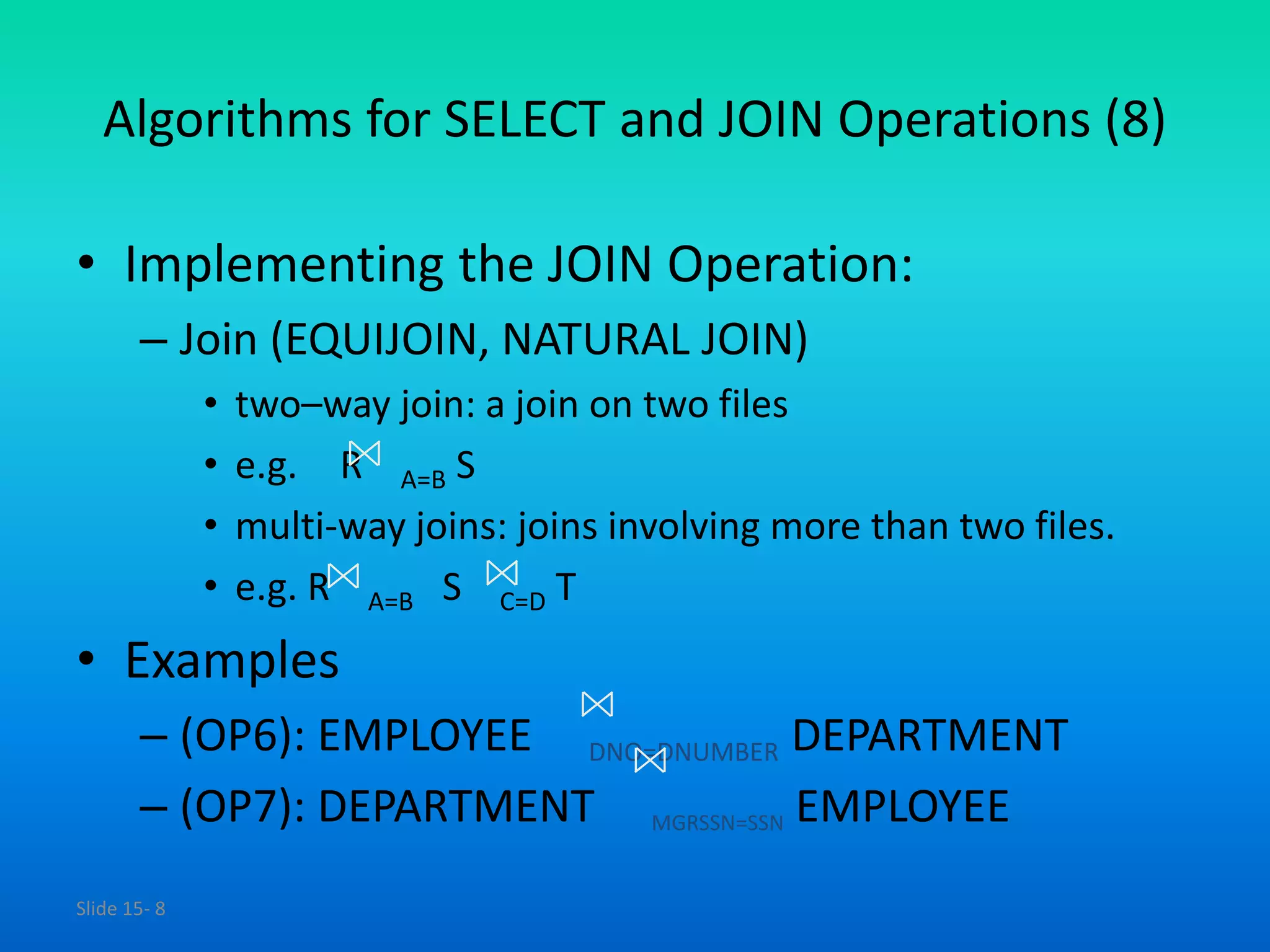
• Implementing the JOIN Operation (contd.):
• Methods for implementing joins:
– J1 Nested-loop join (brute force):
• For each record t in R (outer loop), retrieve every record s from S
(inner loop) and test whether the two records satisfy the join
condition t[A] = s[B].
– J2 Single-loop join (Using an access structure to retrieve the
matching records):
• If an index (or hash key) exists for one of the two join attributes —
say, B of S — retrieve each record t in R, one at a time, and then
use the access structure to retrieve directly all matching records s
from S that satisfy s[B] = t[A].

10. Slide 15- 10
Algorithms for SELECT and JOIN Operations (10)
• Implementing the JOIN Operation (contd.):
• Methods for implementing joins:
– J3 Sort-merge join:
• If the records of R and S are physically sorted (ordered) by value of
the join attributes A and B, respectively, we can implement the
join in the most efficient way possible.
• Both files are scanned in order of the join attributes, matching the
records that have the same values for A and B.
• In this method, the records of each file are scanned only once each
for matching with the other file—unless both A and B are non-key
attributes, in which case the method needs to be modified slightly.

11. Slide 15- 11
Algorithms for SELECT and JOIN Operations (11)
• Implementing the JOIN Operation (contd.):
• Methods for implementing joins:
– J4 Hash-join:
• The records of files R and S are both hashed to the
same hash file, using the same hashing function on the
join attributes A of R and B of S as hash keys.
• A single pass through the file with fewer records (say, R)
hashes its records to the hash file buckets.
• A single pass through the other file (S) then hashes
each of its records to the appropriate bucket, where
the record is combined with all matching records from
R.

12. Slide 15- 12
Algorithms for SELECT and JOIN Operations (12)

13. Slide 15- 13
Algorithms for SELECT and JOIN Operations (13)

14. Slide 15- 14
Algorithms for SELECT and JOIN Operations (14)
• Implementing the JOIN Operation (contd.):
• Factors affecting JOIN performance
– Available buffer space
– Join selection factor
– Choice of inner VS outer relation

15. Slide 15- 15
Algorithms for SELECT and JOIN Operations (15)
• Implementing the JOIN Operation (contd.):
• Other types of JOIN algorithms
• Partition hash join
– Partitioning phase:
• Each file (R and S) is first partitioned into M partitions using a
partitioning hash function on the join attributes:
– R1 , R2 , R3 , ...... Rm and S1 , S2 , S3 , ...... Sm
• Minimum number of in-memory buffers needed for the
partitioning phase: M+1.
• A disk sub-file is created per partition to store the tuples for
that partition.
– Joining or probing phase:
• Involves M iterations, one per partitioned file.
• Iteration i involves joining partitions Ri and Si.

16. Slide 15- 16
Algorithms for SELECT and JOIN Operations (16)
• Implementing the JOIN Operation (contd.):
• Partitioned Hash Join Procedure:
– Assume Ri is smaller than Si.
1. Copy records from Ri into memory buffers.
2. Read all blocks from Si, one at a time and each record
from Si is used to probe for a matching record(s) from
partition Si.
3. Write matching record from Ri after joining to the
record from Si into the result file.

17. Slide 15- 17
Algorithms for SELECT and JOIN Operations (17)
• Implementing the JOIN Operation (contd.):
• Cost analysis of partition hash join:
1. Reading and writing each record from R and S during the
partitioning phase:
(bR + bS), (bR + bS)
2. Reading each record during the joining phase:
(bR + bS)
3. Writing the result of join:
bRES
• Total Cost:
– 3* (bR + bS) + bRES

18. Slide 15- 18
Algorithms for SELECT and JOIN Operations (18)
• Implementing the JOIN Operation (contd.):
• Hybrid hash join:
– Same as partitioned hash join except:
• Joining phase of one of the partitions is included during the
partitioning phase.
– Partitioning phase:
• Allocate buffers for smaller relation- one block for each of the M-1
partitions, remaining blocks to partition 1.
• Repeat for the larger relation in the pass through S.)
– Joining phase:
• M-1 iterations are needed for the partitions R2 , R3 , R4 , ......Rm
and S2 , S3 , S4 , ......Sm. R1 and S1 are joined during the
partitioning of S1, and results of joining R1 and S1 are already
written to the disk by the end of partitioning phase.

19. Assignment
• Explain the Algorithm for SELECT and JOIN
operations