TS Editor 3.0 User Manual

Hydro Office Software for Water Sciences

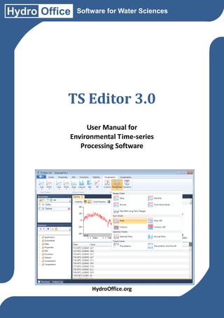
TS Editor 3.0
User Manual for
Environmental Time-series
Processing Software

HydroOffice.org

Gregor M. 2013. TS Editor 3.0 – user manual for environmental time-series processing
Citation:
software. HydroOffice.org, Online Only, 95 p.

© Miloš Gregor, PhD. / milos.gregor@hydrooffice.org
HydroOffice.org – software for water science
This file is published under Creative Common License

1 / 92

Contents at a Glance

1 Introduction ............................................................................................................................................... 7
2 Starting the program .............................................................................................................................. 9

3.1 Ribbon Main Menu ................................................................................................................. 11
3 User Interface of TS Editor ................................................................................................................ 10

3.2 Ribbon Toolbar ........................................................................................................................ 12
3.3 Panels ......................................................................................................................................... 15

4.1 Application ............................................................................................................................... 34
4 Functions ................................................................................................................................................. 33

4.2 Documents ................................................................................................................................ 36
4.3 Data ............................................................................................................................................ 39
4.4 Properties ................................................................................................................................. 42
4.5 Edit ............................................................................................................................................. 48
4.6 Functions .................................................................................................................................. 62
4.7 Statistic ...................................................................................................................................... 67
4.8 Visualization ............................................................................................................................ 74
4.9 Cooperation .............................................................................................................................. 87
5 Conclusion ............................................................................................................................................... 91
Appendix I: Document Naming Conventions ............................................................................... 92

2 / 92

Table of Contents

1 Introduction ............................................................................................................................................... 7
2 Starting the program .............................................................................................................................. 9
3 User Interface of TS Editor ................................................................................................... 10
3.1 Ribbon Main Menu .............................................................................................................. 11
3.2 Ribbon Toolbar ..................................................................................................................... 12

3.3.1 Documents Panel ............................................................................................................... 15
3.3 Panels ....................................................................................................................................... 15

3.3.2 Functions Panel .................................................................................................................. 16
3.3.3 Processes Panel .................................................................................................................. 18
3.3.4 Output Log Panel ............................................................................................................... 19
3.4 Script Window ........................................................................................................................ 19
3.5 Documents ............................................................................................................................... 20
3.5.1 Table........................................................................................................................................ 22
3.5.2 Chart ....................................................................................................................................... 23
4 Functions ................................................................................................................................................. 33

4.1.1 Application.Help ................................................................................................................ 34
4.1 Application ............................................................................................................................. 34

4.1.2 Application.Minimize....................................................................................................... 34
4.1.3 Application.Restore .......................................................................................................... 34
4.1.4 Application.Maximize ...................................................................................................... 34
4.1.5 Application.About ............................................................................................................. 34
4.1.6 Application.End.................................................................................................................. 34
4.1.7 Application.Functions ...................................................................................................... 34
4.1.8 Application.Processes...................................................................................................... 35
4.1.9 Application.Log .................................................................................................................. 35

4.2.1 Documents.Show ............................................................................................................... 36
4.2 Documents .............................................................................................................................. 36

4.2.2 Documents.ShowAll .......................................................................................................... 36
4.2.3 Documents.Close ................................................................................................................ 36
4.2.4 Documents.CloseAll ........................................................................................................... 36
4.2.5 Documents.Edit .................................................................................................................. 36
4.2.6 Documents.Delete .............................................................................................................. 37
4.2.7 Documents.DeleteAll ........................................................................................................ 37
4.2.8 Documents.Rename .......................................................................................................... 37
4.2.9 Documents.Comment ....................................................................................................... 37
4.2.10 Documents.SelectAll ....................................................................................................... 37
4.2.11 Documents.InvertSelection .......................................................................................... 37
4.2.12 Documents.SeriesType ................................................................................................. 38

4.3.1. Data.Open ............................................................................................................................ 39
4.3 Data ........................................................................................................................................... 39

4.3.2. Data.Create .......................................................................................................................... 39
4.3.3. Data.Save .............................................................................................................................. 41

4.4.1 Properties.NumberOfRecords....................................................................................... 42
4.4 Properties ............................................................................................................................... 42

4.4.2 Properties.NumberOf....................................................................................................... 42
4.4.2.1 Properties.NumberOf.EmptyValues ........................................................................ 42

3 / 92

4.4.2.2 Properties.NumberOf.ZeroValues ............................................................................ 43
4.4.2.3 Properties.NumberOf.DefinedValues ..................................................................... 43
4.4.3 Properties.TimeRanges................................................................................................... 43
4.4.4 Properties.Gaps .................................................................................................................. 43
4.4.4.1 Properties.Gaps.Annual ............................................................................................... 44
4.4.4.2 Properties.Gaps.Monthly............................................................................................. 44
4.4.4.3 Properties.Gaps.Daily ................................................................................................... 44
4.4.4.4 Properties.Gaps.Weekly ............................................................................................... 44
4.4.4.5 Properties.Gaps.Hourly................................................................................................ 44
4.4.4.6 Properties.Gaps.UserDefined .................................................................................... 45
4.4.5 Properties.IsContinual..................................................................................................... 45
4.4.6 Properties.HasUniformStep........................................................................................... 46
4.4.7 Properties.ShowTimeSteps ........................................................................................... 46
4.4.8 Properties.IncreasingSegments ................................................................................... 46
4.4.8.1 Properties.IncreasingSegments.AverageLength ................................................ 46
4.4.8.2 Properties.IncreasingSegments.Length................................................................. 47
4.4.8.3 Properties.IncreasingSegments.TotalLength ....................................................... 47
4.4.8.4 Properties.IncreasingSegments.Count ................................................................... 47
4.4.9 Properties.ConstantSegments ....................................................................................... 47
4.4.10 Properties.DecreasingSegments................................................................................ 47

4.5.1 Edit.Select ............................................................................................................................. 48
4.5 Edit ............................................................................................................................................ 48

4.5.1.1 Edit.Select.ByTimeRange ............................................................................................ 48
4.5.1.2 Edit.Select.ByTimeFilter .............................................................................................. 49
4.5.1.3 Edit.Select.ByValueRange ............................................................................................ 50
4.5.1.4 Edit.Select.ByConditions.............................................................................................. 50
4.5.1.5 Edit.Select.ByCourse ..................................................................................................... 50
4.5.1.5.1 Edit.Select.ByCourse.Increasing ........................................................................... 51
4.5.1.5.2 Edit.Select.ByCourse.Constant ............................................................................... 51
4.5.1.5.3 Edit.Select.ByCourse.Decreasing .......................................................................... 51
4.5.1.6 Edit.Select.EmptyValues ............................................................................................... 51
4.5.1.7 Edit.Select.ZeroValues .................................................................................................. 51
4.5.2 Edit.Update ........................................................................................................................... 51
4.5.2.1 Edit.Update.+ ................................................................................................................... 51
4.5.2.2 Edit.Update.-..................................................................................................................... 52
4.5.2.3 Edit.Update.* .................................................................................................................... 52
4.5.2.4 Edit.Update./ .................................................................................................................... 52
4.5.2.5 Edit.Update.Math............................................................................................................ 52
4.5.3 Edit.Delete ............................................................................................................................ 52
4.5.4 Edit.Gaps ............................................................................................................................... 53
4.5.4.1 Edit.Gaps.Fill .................................................................................................................... 53
4.5.4.2 Edit.Gaps.FillByComparing ........................................................................................ 54
4.5.5 Edit.Transform ................................................................................................................... 54
4.5.5.1 Edit.Transform.Weekly.ToDaily ................................................................................ 55
4.5.5.2.1 Edit.Transform.Daily.ToWeekly ............................................................................ 55
4.5.5.2.2 Edit.Transform.Daily.ToHourly ............................................................................. 55
4.5.5.3.1 Edit.Transform.Hourly.ToDaily ............................................................................. 55
4.5.5.3.2 Edit.Transform.Hourly.ToHMS .............................................................................. 57
4.5.5.4 Edit.Transform.HMS.ToHourly ................................................................................. 57
4.5.5.5 Edit.Transform.UserDefined...................................................................................... 57
4.5.6 Edit.ShiftInTime................................................................................................................. 58

4 / 92

4.5.7 Edit.ShowAsTimeSpan .................................................................................................... 58
4.5.8 Edit.GetTimeStructure ..................................................................................................... 58
4.5.9 Edit.GetValues ..................................................................................................................... 59
4.5.11 Edit.Convert ...................................................................................................................... 60

4.6.1 Functions.MassCurve ....................................................................................................... 62
4.6 Functions................................................................................................................................. 62

4.6.1.1 Functions.MassCurve.Single ....................................................................................... 62
4.6.1.2 Functions.MassCurve.Double .................................................................................... 63
4.6.2 Functions.SeriesInterpolation ...................................................................................... 63
4.6.3 Functions.CompositeTable ............................................................................................. 64
4.6.4 Functions.UniteSeries ...................................................................................................... 64
4.6.5 Functions.ProfileInTime ................................................................................................. 65

4.7.1 Statistic.Basic ....................................................................................................................... 67
4.7 Statistic ..................................................................................................................................... 67

4.7.1.1 Statistic.Basic.Min .......................................................................................................... 67
4.7.1.2 Statistic.Basic.Max .......................................................................................................... 67
4.7.1.3 Statistic.Basic.Avg ........................................................................................................... 67
4.7.1.4 Statistic.Basic.Sum ......................................................................................................... 68
4.7.1.5 Statistic.Basic.Count ...................................................................................................... 68
4.7.2 Statistic.InTime ................................................................................................................... 68
4.7.2.1 Statistic.InTime.Annual ................................................................................................ 68
4.7.2.1.1 Statistic.InTime.Annual.Min .................................................................................... 68
4.7.2.1.2 Statistic.InTime.Annual.Max ................................................................................... 68
4.7.2.1.3 Statistic.InTime.Annual.Avg .................................................................................... 69
4.7.2.1.4 Statistic.InTime.Annual.Sum................................................................................... 69
4.7.2.1.5 Statistic.InTime.Annual.Count................................................................................ 69
4.7.2.2 Statistic.InTime.Seasonal ............................................................................................ 69
4.7.2.2.1 Statistic.InTime.Seasonal.Min ................................................................................ 69
4.7.2.2.2 Statistic.InTime.Seasonal.Max ................................................................................ 69
4.7.2.2.3 Statistic.InTime.Seasonal.Avg ................................................................................. 70
4.7.2.2.4 Statistic.InTime.Seasonal.Sum ............................................................................... 70
4.7.2.2.5 Statistic.InTime.Seasonal.Count ............................................................................ 70
4.7.2.3 Statistic.InTime.Monthly ............................................................................................. 70
4.7.2.3.1 Statistic.InTime.Monthly.Min ................................................................................. 70
4.7.2.3.2 Statistic.InTime.Monthly.Max ................................................................................. 70
4.7.2.3.3 Statistic.InTime.Monthly.Avg .................................................................................. 70
4.7.2.3.4 Statistic.InTime.Monthly.Sum ................................................................................ 70
4.7.2.3.5 Statistic.InTime.Monthly.Count ............................................................................. 71
4.7.3 Statistic.Specialized.Reports ........................................................................................... 71
4.7.3.1 Statistic.Specialized.Reports.Monthly ..................................................................... 71
4.7.3.3.1 Statistic.Specialized.Reports.Monthly.Min ......................................................... 72
4.7.3.3.2 Statistic.Specialized.Reports.Monthly.Max ......................................................... 72
4.7.3.3.3 Statistic.Specialized.Reports.Monthly.Avg .......................................................... 72
4.7.3.3.4 Statistic.Specialized.Reports.Monthly.Sum ........................................................ 72
4.7.3.3.5 Statistic.Specialized.Reports.Monthly.Count ..................................................... 72
4.7.3.2 Statistic.Specialized.Reports.Classic.AnnualTable ............................................... 72

4.8.1 Visualization.FastCharts ................................................................................................. 74
4.8 Visualization .......................................................................................................................... 74

4.8.1.1 Visualization.FastCharts.Line .................................................................................... 75
4.8.1.2 Visualization.FastCharts.Point .................................................................................. 75

5 / 92

4.8.2 Visualization.ClassicCharts............................................................................................. 75
4.8.2.1 Visualization.Classic Charts.Line .............................................................................. 75
4.8.2.2 Visualization.ClassicCharts.Point ............................................................................. 76
4.8.2.3 Visualization.Classic Charts.Area ............................................................................. 76
4.8.2.4 Visualization.Classic Charts.Bar................................................................................ 76
4.8.2.5 Visualization.Classic Charts.Column ....................................................................... 76
4.8.2.6 Visualization.ClassicCharts.XY .................................................................................. 77
4.8.3 Visualization.SpecializedCharts ................................................................................... 77
4.8.3.1 Visualization.SpecializedCharts.Custom ............................................................... 77
4.8.3.2 Visualization.SpecializedCharts.Predefined ......................................................... 78
4.8.3.2.1.1 Visualization.SpecializedCharts.Predefined.RangeCharts.Daily ............ 79
4.8.3.2.1.2 Visualization.SpecializedCharts.Predefined.RangeCharts.Monthly ...... 79
4.8.3.2.1.3 Visualization.SpecializedCharts.Predefined.RangeCharts.Annual ........ 79
4.8.3.2.1.4 Visualization.SpecializedCharts.Predefined.RangeCharts.
FromMoreSeries ........................................................................................................................... 79
PartWithLong- TermRanges ................................................................................................... 80
4.8.3.2.2 Visualization.SpecializedCharts.Predefined.SumCharts ............................... 80
4.8.3.2.2.1 Visualization.SpecializedCharts.Predefined.Sum Charts.Area ................ 81
4.8.3.2.2.2 Visualization.SpecializedCharts.Predefined.SumCharts.Area100 ......... 81
4.8.3.2.2.3 Visualization.SpecializedCharts.Predefined.SumCharts.Column ........... 81
4.8.3.2.2.4 Visualization.SpecializedCharts.Predefined.SumCharts.Column100 ... 81
4.8.3.2.3 Visualization.SpecializedCharts. Predefined.SelectionCharts ..................... 82
4.8.3.2.3.1 Visualization.SpecializedCharts.Predefined.SelectionCharts.
SelectedParts .................................................................................................................................. 82
AnnualParts .................................................................................................................................... 83
4.8.3.2.4 Visualization.SpecializedCharts.Predefined.TypedCharts ........................... 83
4.8.3.2.4.1 Visualization.SpecializedCharts.Predefined.TypedCharts.
Precipitation ................................................................................................................................... 83
PrecipitationAndRunoff ............................................................................................................. 84
4.8.3.3 Visualization.SpecializedCharts.Dynamic............................................................. 85

4.9.1 Cooperation.Software.Feflow ........................................................................................ 87
4.9 Cooperation............................................................................................................................ 87

4.9.1.1 Cooperation.Software.Feflow.ReadFeflowTimeSeries ...................................... 88
4.9.1.2 Cooperation.Software.Feflow.CreateFeflowTimeSeries ................................... 88
4.9.2 Cooperation.File.CSV ........................................................................................................ 89
4.9.2.1 Cooperation.File.CSV.ReadCSVFile ........................................................................... 89
4.9.2.2 Cooperation.File.CSV.CreateCSVFile ........................................................................ 90
5 Conclusion ............................................................................................................................................... 91
Appendix I: Document Naming Conventions ............................................................................... 92

6 / 92

1 Introduction
This is the user manual for the TS Editor tool in version 3.0. The program name was created
from the words “Time Series Editor”, which implies its focus and specialization. The first two
versions were developed by the author for personal use especially in areas where computing
capabilities of other applications, such as MS Excel and other spreadsheets or statistical packages,
were insufficient. These versions were used for more narrowly focused operations (Fig. 1).
Gradually, development of HydroOffice package enabled data preparation in the form of time series
for each of its applications and provided result processing and visualization.
Therefore, it was decided to finalize this application to the stage where it is offered as a
separate installable tool. In the progress, this tool has been re-programmed with its architecture,
functionality and scope completely redesigned. All information and instructions contained in the
previous programs are incorporated in this new development, thus making this the most
sophisticated and useful tool in the HydroOffice software package. This program reads data from
files much faster and the calculation speed and visualization features are significantly superior to
other systems. This was achieved through the use of new technology and programming techniques.
However, since this program has not been optimized to run on Windows XP, for best results it must
be run on the newer operating system of MS Vista/7/8.

Fig. 1: TS Editor in versions 1.0 and 3.0.

The following text describes the functionality of this program, the user interface and
possibilities and limitations for its use. If you work in the field of hydrology, hydrogeology,
meteorology or climatology, this program is designed for you. It saves time spent in processing data
such as measured values of river discharges, springs’ yields, observed groundwater level changes,
air temperatures, precipitation and wind speed/directions. This TS Editor 3.0 latest version offers
over 2,000 functions which can be combined in different ways. You have vast possibilities
immediately you understand the principles of working with this program. All functions are run
using the buttons in the menu, from the functional tree to specialized applications, and this program
includes a very simple scripting interface. This not only makes your work much quicker and easier

7 / 92

but it also especially focuses on features lacking in other programs. Please check out the following
options and functionality.
I am sure that this program will simplify your work, and if you have problems using it,
please feel free to contact me in the forum section on the web (http://hydrooffice.org), or please
email me. I will be extremely grateful for your comments, questions and future references.

8 / 92

2 Starting the program
Program TS Editor 3.0 is not distributed as separate software, but as a part of HydroOffice
2012 software (Fig. 2).

Fig. 2: Main window of HydroOffice 2012 software with the TS Editor 3.0 tool.

It is therefore installable and executable as other tools of the HydroOffice package and if
you have purchased a license for its use, its installation option appears in the list of installable tools.
The overall process of purchasing, licensing, installation and startup of the program is described in
the separate user manual for using the HydroOffice 2012 software. Therefore, at this point the
process is not described in deeper detail. If, you have not purchased a licence for TS Editor 3.0, you
can always buy it at http://hydrooffice.org , or at your dealer.

TIP: If you wish to try the program before buying it, you can install the “Demo”
Version. This version includes all the functionality of the program. Its only limitation is that for
test purposes you can only use time series which are automatically loaded into the program.
Your processed results can be exported from the program without any restrictions.

9 / 92

3 User Interface of TS Editor
The program user interface was developed using the latest technology and practices, and it
consists of three main parts – The Ribbon, and the Panels and Documents Area (Fig. 3).

Fig. 3: Main window of TS Editor 3.0.

The basis of the program window is Ribbon (Fig. 3). This software element is relatively
new, but when users adopt it, this layout allows relatively quick and efficient work with the program.
Ribbon is located at top of the window. Almost all program functions are hidden under individual
Tabs. The core functionality for working with TS Editor is grouped on the Home tab and all other
functions are divided into separate logical categories on the remaining tabs. In addition, it is also
possible to control the functions from the functional tree in the panel named Functions. This
operation of this feature is further explained in chapter 3.3.2.
The second part of the program consists of separate panels on the left side of the window
(Fig. 3). These panels can be relocated by the user in a window, separate to the main window, with
“hide” and “close”. The only panel which cannot be closed is the Documents panel which is a
permanent part of the program. After starting the program, there are two panels docked in the right
window pane (the Documents and Functions panels), and two more are docked at the bottom edge
of the window (Processes and Output Log). These two latter panels have an AutoHide parameter
set to “TRUE”, which means that if they aren't active, or the user does not focus on them with the
mouse, they are automatically hidden. A functionality description of these panels is described in
chapters 3.3.1 – 3.3.4.
The last and largest part of the program window is designed to display separate documents.
When the user loads input files or processes, the required calculation, results are shown in this
section. Similar to the panels, all individual documents can be shown, docked in the main window,
switched between each other, re-located from the main window into separate windows and closed.
These functions are all described in detail in the following sections of the manual.

10 / 92

3.1 Ribbon Main Menu
The basis of the TS Editor 3.0 user interface is ribbon. It has a privileged status-control
called the Ribbon Main Menu button (Fig. 4a). Clicking this shows all basic functions of the
program (Fig. 4b). The first option is to show the user manual in PDF format. The second item
displays basic information about the program and licence. The HydroOffice Online command
shows the project website. This feature is similar to the one in the basic HydroOffice 2012 program.
When you click on the last item named Settings, the option for user interface settings is displayed.
The current version allows you to set only two parameters of user interface – visibility of the ribbon
toolbar and setting for functions dialogs

Fig.4: Ribbon Main Menu in TS Editor 3.0 (A – Ribbon Main Menu button; B – Functions of the Ribbon
Main Menu).
The window shown
in Figure 5 appears when
you click on Settings >
Ribbon. You can set the
visibility of the ribbon
toolbar in this window, and
this setting has two states.
The first option is to have
the ribbon toolbar entirely
visible so that the applica-
tion appears exactly at it
does when you start the
Fig. 5: Window for Ribbon toolbar visibility setup. program. In this state, the
ribbon automatically hides
and the program is visually
similar to older software
types based on menu control.
In this case, automatically
selected functions will be
displayed when you click on
Fig. 6: Dialog for setup of the AutoClose parameter for functions the selected item in the
dialogs. menu. But when you focus
on a different part of the
window, the toolbar is automatically hidden. This option is appropriate for use if you have small
screen resolution, or if you want to see multiple documents in parallel.
When you click on the second item, Settings > Runtime Functions Window, the window

11 / 92

shown in Figure 6 appears. With this function you can set the parameter AutoClose for functions
dialog. Default value is “TRUE”. This setting is used for a specific purpose. If you click any
function under AutoClose, a separate dialog is shown for setting parameters called “function”. After
setting these parameters and further processing of “function”, these windows can be automatically
closed or they can be preserved for changing parameters of the function and re-launching. If this
AutoClose parameter is set to “true”, the windows automatically close after the first execution of
the function. However if you want the window to remain open, you set this parameter to “FALSE”,
so that the window will not close and you can execute the selected function again. The function of
this AutoClose parameter will become clearer after reading this manual, If you have any difficulty
in understanding its function you can run some functions under both states (AutoClose = TRUE /
FALSE) and the difference will be apparent.

3.2 Ribbon Toolbar
As mentioned earlier, all the functions for time series processing are in the ribbon toolbar in
the main program window. All ribbon tabs are highlighted in Figure 7. Overall, functions are
divided into seven tabs. The first Tab – Home - displays functions for individual application Panels,
importing / exporting data and manual definition of time series plus features for working with
individual documents.
Using functions on the Properties tab allows the user to acquire the basic technical and
structural information about the selected time series (meta-data), such as the total number of records,
the number of records satisfying a special condition, determining the time range of the series, the
gaps in time series, information on the uniformity and continuality of the document and information
about increasing, decreasing and constant segments of your values.
Functions of the Edit tab are used to edit the actual time series. With these features it is
possible to filter the data using multiple methods and approaches, in bulk edit values or to delete
them. Additional features allow you to fill gaps in time, transform the time series, move the values
in time and to convert units or to combine two series into a single series.
The tab Functions contains specialized functions, including the calculations of single or double
mass curves, linear interpolation of time series, creation of a single table from multiple time series,
document unification on the basis of the one selected or visualization of time series in the profile
(examples of this are; the relationships between ‘water temperature and the depth of a well’ or
between ‘precipitation and altitude’).
Functions on the Statistic tab are prepared for variable statistical processing of values in
time series. Examples include – ‘monthly averages, annual maximums, long-term minimums and
seasonal statistical characteristics’. In addition, this tab includes functions for automatic production
of various statistical reports to be used in final reports and articles.
The penultimate tab – Visualization - contains functions for visualizing the time series. The
program allows you to create highly variable time series visualizations, to form simple line charts in
predefined range charts or rainfall-runoff graphs.
The last tab is - Cooperation - which contains tools for working with external programs and
files. The current version of TS Editor includes features for co-working with the hydraulic model
‘Feflow’. The program allows you to import data from Feflow or to export data from the application
into formats supported by Feflow software. The last feature is a function to import /export data from
/in the CSV format (comma separated values).

TIP To quickly switch between individual ribbon tabs, focus the mouse on ribbon and
rotate the wheel on the mouse. This is a little- known trick to quickly switch ribbon tabs. :-)

12 / 92

Fig. 7: Ribbon toolbar with all the functions.

The Ribbon toolbar is not as static as it appears. The character and structure is
fundamentally changed when you double-click on the graph in your document (Fig. 8). After
double-clicking, the basic functions of the program are hidden, but the functions for visual setting
of your selected graph appear.
Individual tabs of the ribbon toolbar are shown in Figure 9. The Main tab contains the basic
settings of the chart together with the functions for graph export to an image file, or the option of
direct printing. The second tab called Background includes options for setting the chart
background. Using functions in the next tab allows you to setup chart area properties, and the
functions for setting axis properties are listed on the following tab. The Legend tab allows you to
set properties in the chart legend. The next tab contains a collection of settings for individual graph
series, and using functions on the last tab lets you define, align, adjust and set your graph titles.
A complete description of all the features and how to set up the chart will be explained in a
separate chapter (3.5.2). If you want to hide tabs for chart visual setting and show the basic
functions of the application, just activate a different part of the window by clicking on any panel, or
click on the first button displayed on each tab - called “Close”.

13 / 92

Fig. 8: Ribbon toolbar structure after double-clicking on the chart in the displayed document.

Fig. 9: Ribbon toolbar tabs for configuration of the chart’s visual properties.

14 / 92

3.3 Panels
The panels form a very important part of the program because most work in the program is
performed through them. After starting the program, two of these are docked on the left side of
window and two are docked on the bottom edge of the window and are automatically minimized.
This chapter now explains their functionality and importance. As the first the Documents Panel is
presented first. In this panel, the user has access to all documents that were imported into the
program or generated by the selected function. This is followed by the Functions Panel where all
application functions are displayed in a tree structure. Finally, the assistance Panels named
Processes and Output Log are introduced.

3.3.1 Documents Panel

The Panel titled Documents (Fig. 10 a) is one of the most important panels in the program,
because all documents stored in computer memory are listed therein. Therefore, this panel can not
be closed, only relocated or minimized. Individual documents are displayed as items in the list.
Each document is represented as an individual item in one line and is presented by three elements.
The first element is an icon. This icon defines the document type. When this icon has a small arrow,
this means that the document has been loaded from the file onto the disk. If the icon is displayed
with a small “plus” picture the document was created directly inside the program using any function
on the selected document. This icon is followed by a letter that defines the type of time series stored
in the document. If the document does not have this letter, it means that the document does not have
the time series character. One example of such a document could be a result table with calculated
statistical parameters. Determination of the document type is carried out automatically, and the
document can be defined by the letter W (weekly time series), D (daily time series), H (hourly time
series) and finally U (undetected time series). The name of document is displayed after these two
icons, and the given document name must be unique for this list.
This panel also contains five
commands in the toolbar (Fig. 10 b). With
the first three buttons, you define which
documents you want to see. You have the
following choices; (1) display all
documents in memory, (2) display only
those which have been loaded from
computer disk, or (3) display only those
which were created directly in the program
using its built-in functionality.
You must be certain which of these
documents you wish to use before you
perform a program function. Then, you
click on the document to be used and select
the required function from the ribbon
toolbar. Now the fourth and fifth toolbar
commands come into play. If you want to
use a function for multiple documents
Fig. 10: Panel Documents (Left – general view of the simultaneously, press the Ctrl or Shift key
panel; Right – description of the panel toolbar and click on all the required documents.
commands). Using this approach, you can process
multiple documents simultaneously. If you
want to select all the documents at once, click on the penultimate button in the toolbar. If you want
to invert the document selection, click on the last button.

15 / 92

After selecting the documents and clicking on the desired function, one or more new
documents will be created containing your result. Processed results immediately appear in separate
document windows. These windows can be closed, but they are still retained in the memory. If you
want to see them again, just double click on the selected document in the panel and it will be
displayed in a separate window. If you keep the mouse over the document, tooltip information for
the document will be displayed (Fig. 11).
This element shows information about
the document. (1) The first line contains the
name of the document (2) the second details
the primary file source it is based on, (3) the
third line shows the time stamp, which
defines the time when the document was
loaded into memory, (4) If the selected
document is created from another document
using any built-in function, its name appears
Fig. 11: Tooltip information for the selected on the fourth line, and (5) The function used
document. is recorded on the fifth line. Finally, if the
program or user has added comments to the document, these are displayed on the last line.
The following features of this panel appear when you right-click the mouse on the selected
document (Fig. 12).
By clicking on the first menu item
(Show), the user can view the selected
document in a separate window. The second
item is used for manual editing of the selected
document. You must take care when editing,
because you directly edit the document in
memory without cancelling the changes. The
Delete command can immediately delete the
document from computer memory. The
Rename command changes the name of the
selected document. The menu item called
Fig. 12: Popup menu items for the selected
Series Type is used to change the time series
document.
type if the program has determined it
incorrectly. The Comment command enables you to manually assign comments to the document,
and these are then displayed in the tooltip information (Fig. 11). Finally, the last command allows
you to select all documents in memory.

TIP At work it is very important to know how you have named your documents,
especially for documents that are generated directly in the program. Appendix 1 details
Document Naming Conventions.

3.3.2 Functions Panel

The second panel is called Functions (Fig. 13). This panel contains every function of the TS
Editor 3.0 software in a tree structure.
Exactly as you found in the ribbon toolbar, all functions in this panel are divided into logical
groups. The only difference here is that the functions from the ribbon Home tab are divided into
three different groups, namely Application, Documents and Data. The remaining basic tree items
are the same as those in the ribbon tabs headers. The individual functions were described according
to this tree structure in the previous chapter - Chapter 4. The user can choose whether to run the
required functions from the ribbon toolbar or from this panel, or to use a combination of both.
Figure 13 defines the commands from the panel toolbar. The first button serves to expand the tree

16 / 92

levels. Each click on this
button expands the next
tree level. Activating the
second button collapses the
tree, and immediately
following the first click the
tree is collapsed at the
highest level. The third
command runs a function
defined by selecting the
tree item or entering script
into the text box. The script
text box can be hidden or
displayed using the last
button, and Figure 14
shows how the panel looks
when the script text box is
displayed or hidden.
Fig. 13: Panel Functions (Left – general view of the panel; Right – You can launch the
description of the panel toolbar commands). function you wish to run
by writing it in the script
text box, and the text box
will then automatically
complete the name of the
desired function (Fig. 15).
The function of the
last button on the toolbar is
Fig. 14: Displayed (Left) and hidden (Right) script text box. now explained. This “Coo-
peration” button is used to
display the Info bar that serves as a help for the selected function (Fig. 16). When you click on the
selected item in the tree you automatically loads its name and description.

Fig. 15: Auto-completion functionality Fig. 16: Panel Information bar.
of the script text box.

A second method for obtaining information about the selected item in the tree is to keep the
mouse cursor over it until the tooltip is displayed (Fig. 17). This program function can be run in
three ways. (1) You can double-click on the selected item in the tree, (2) you can press the F5 key
after writing your script in the text box or (3) you can press the third button in the panel toolbar.
Using this panel is quite simple, but detailed description of the individual functions is contained in
chapter 4.

17 / 92

TIP : As explained in the
previous text, you can run the functions
by using the ribbon toolbar buttons or by
using the items on this panel. In addition,
TS Editor 3.0 includes a specialized
option for professionals - the “command
Fig. 17. Tooltip help for the selected tree item. line” - which is described in the sub-
chapter “Scripts Window”.

3.3.3 Processes Panel

The first two panels are minimized in the bottom left corner of the application (Fig. 18), and
the structure and properties of the Processes panel are now described.

Fig. 18: Minimized application Panels.

The Processes panel stores the history of your used functions and documents. If you want to
view this panel, click on its header. This panel is always empty when you run the application (Fig.
19).

Fig. 19: Empty Processes panel after application start.

When you import multiple files into the program and you process them by selected functions,
the table is filled with information (Fig. 20). The table consists of four columns. The first column
(ID) defines the number of the process. The second column (Source) defines the document or file
on your computer disk used in your actual processing. Your existing file name, or the new file name
you give it, and its directory path appear in this cell.
The third column (Function) defines the name of function used in your current process - for
example; Data.Open. The last column (To Document) defines the name of the document created
by a given function in your current process. Using this table, you can also control how individual
documents are created in the program (from document or file >>> by function >>> to document).
The example, Figure 20 shows that two files were imported into the program using the
Data.Open function. The names of these documents are Q1 and Q2. Subsequently, the following
two functions were performed on document Q1; (1) Annual maximum values were calculated from
the time series and the result is stored in document Q1.3, and (2) the average monthly values and
the result are stored in document Monthly_Avg.4.

18 / 92

Fig. 20: Processes panel with the history of used functions and documents.

One advantage of storing this history is that when you import multiple files into the program
you can check for gaps in your data, find missing values and create statistical results based on these
documents. Using this panel you can therefore create a large number of new documents without
losing track of their process history.

3.3.4 Output Log Panel

The final panel of the TS Editor 3.0 is the Output Log panel (Fig. 21). This contains only a
simple text box where application logs are stored. Each record has the time you created it, its type
and the log message.

Fig. 21: Screenshot of the Output Log panel.

The log type is labelled with OK or Error. If the type is OK, this shows that the process,
function or initialization was without any detected error. The Error label indicates that an error
occurred in the process. The log message then contains information such as the name of the
function which created the error message or a detected bug. In addition to automatically generated
logs, you can also add comments or notes here.

3.4 Script Window

The command line in this program called Script Window has a very useful function (Fig.
22). When you use TS Editor on a daily basis, you will quickly know the required commands
because they are simple, logical and self explanatory. The command line tool is implemented in this
program for professional users.

19 / 92

Fig. 22: Screenshot of the Script Window.

You use this tool by pressing the hot key CTRL+F, and a new window appears containing a
simple text box where you enter your script command. When you begin typing a command, the text
program automatically scans more than 2,300 commands and displays all options to complete your
demand. This script text box operates differently to the one in the Functions panel. In this script
text box you only need to write the first fragment of your command and the program scanning-
display allows you to select any command similar to your requirement. Figure 23 provides an
example.

Fig. 23: Example from the auto-complete command process.

If you imagine that you want to determine the maximum monthly values in a selected
document, you don't need to write the whole command Statistic.InTime.Monthly.Max. You can
simply write the string 'max', and the program automatically finds all commands that contain this
string and displays them in a drop-down list. You select the one you want and press the F5 key. The
program checks that the command is entered correctly, and if it is, the program closes the window
and runs the desired function.

3.5 Documents

The most important elements of the user interface are documents. As mentioned previously,
the data contained in your documents is stored in computer memory. This may consist of a time
series of values or a table with processed results. These data objects can be visualized in the form of
documents. The example in Figure 24 shows three documents displayed in three separate windows.
The currently visible document is named Q1. The document itself consists of three elements –
toolbar with functions, plus a table and graph. This example shows a document containing a time
series of values for the course of river discharges. The first of the table’s two columns stores the
date-time values and the second column has the actual measurements. The second part of the
window displays the data as a linear graph of values over time.
Documents are automatically listed as tabs, and individual documents can be activated by
clicking on the document header. A second method of switching the visible documents is by holding
down the CTRL key and pressing the TAB key (Fig. 25).
Documents are automatically listed as tabs, and individual documents can be activated by
clicking on the document header. A second method of switching the visible documents is by holding
down the CTRL key and pressing the TAB key (Fig. 25).
In addition to automatic document tabbing, you can switch, dock and align individual
documents. Figure 26 shows examples of working with documents. The left-hand example shows
document separation from the main application window into a separate window, while the one on
the right shows multiple documents in parallel display and alignment in one window, so they are all
visible together.

20 / 92

Fig. 24: Example of an opened document in the program.

Fig. 25: Document-switching using the CTRL+TAB hot-key.

Fig. 26: Moving document (Left) and parallel view of multiple documents on the screen (Right).

A separate part of the document features the toolbar (Fig. 27). Using this toolbar you can set
the graph and table visibility with the first two buttons below.

21 / 92

Examples of these settings
can be seen in Figure 28. With these
Fig. 27: Toolbar from the document window. two buttons, you show or hide the
table and graph so that either
element fills the entire document. In “document display” both elements are visible in the document
area. The only two application functions that generate documents without graphs are “IsContinual”
and “HasUniformStep”. All other functions create table and graph visualization.

Fig. 28: Options for table and graph display in the document (Left – table and graph parallel display;
Middle – hidden table; Right – hidden chart).

Besides this op-
tion of hiding selected
objects in the document,
other toolbar buttons can
alter their position. An
example is shown in
Figure 29 where the chart
can be dragged horizon-
tally or vertically before
or after the table.
Additional
methods of document tab-
le and graph control are
explained in the next two
subsections

Fig. 29: Chart setting options to position the table.

3.5.1 Table

The table has less processing
capabilities than the graph because the
table view is not editable and it only
allows values of the time series or
calculated parameters to be shown.
Basically, data in the table can only be
saved or copied to clipboard (Fig. 30).
Right-click on the table and a pop-
Fig. 30: Working with the table in a selected document. up menu appears showing the above
described functions. If you copy the table
to the clipboard, you can directly insert it into another program such as MS Excel. Otherwise, using
the ‘save’ command stores your data on disk, and its function is identical to Data.Save which is
shown on Figure 38.

22 / 92

3.5.2 Chart

Graphic sections of the documents are more diverse and offer more customization.
Examples of graphs in TS Editor are shown in Figure 31. Each program function which creates a
new document also contains a precisely defined graphic visualization.

Fig. 31: Examples of graphic visualizations in TS Editor.

Only two features in a document graph can be controlled. You can zoom or scroll a selected
part of the graph or activate functions to set the graphic properties. Examples of zooming and
scrolling are shown in Figure 32.

Fig. 32: Example of graph zooming and scrolling.

This figure graphs a time series of temperature measurements over an extended period. If
you want to display only a selected part of this period, press the left mouse button and select the
section you want to view (Fig. 32 Left). When selected, leave the mouse button and the selected
part is displayed separately (Fig. 32 Right). This procedure can be repeated as long as you see only
the part you exactly want to see. Use the scrollbar on the bottom axis and move over the “time”. If
you want to return to the previous scale of display, just click on the small button located to the left
of the scrollbar on the X-axis. Using this method, graphs in documents can be zoomed and scrolled
only over the X-axis. However, it is possible to zoom and scroll graphs over both X and Y axes
using the function group called Visualization. An example is shown in Figure 33.

23 / 92

Fig. 33: Example of graphs that can be zoomed and scrolled on both axes.

These documents don't contain the table portion and therefore they are not listed in the
Documents panel. In addition, all have the same header – Visualization- and under this option, any
parts of your graph can be zoomed. The visual properties of chart are chosen by double-clicking on
the chart area, thus changing the ribbon toolbar as seen in Fig. 34.

Fig. 34: Functions for setting the graph’s visual properties.

This double-click hides the classic functions of the program, and graph setting options are
displayed. These settings are grouped in seven ribbon tabs, and the available options allow you to
completely adjust the visualization. You will appreciate that this software is a very powerful
visualization tool. An example of what can be done with the graph is shown in Figure 35. This
visualization was created by several “tricks” and when you become conversant with working with
all graph properties functions, you will have no problem in creating your own similar graph. These
tricks comprise; (1) visualization of two documents created in one window, and (2) the background
is composed by changing the image and position of chart areas and also changing their size and
transparency.
The following text describes the functionality of each button in the ribbon toolbar. It begins
with examining the settings and functions offered by the Main ribbon tab (Fig. 36).
The following text describes the functionality of each button in the ribbon toolbar. It begins
with examining the settings and functions offered by the Main ribbon tab (Fig. 36).
Figure 36 shows four buttons for setting complete graph properties. The graph ribbon
toolbar itself does not contain all functions and settings you can use for working with graphs.
Although the major commands are included, for some purposes you may need additional commands
which are available using the following four buttons in the ribbon toolbar.
With these settings, you can edit individual Chart Areas, Legends, Chart Titles and Series.
Clicking on any of these buttons displays their properties in a new window (Fig. 37). This window
consists of three parts – (1) the ‘combo’ (combination) box is at the top, (2) the property grid is in
the middle and (3) the label is at the bottom. When the selected graph contains a number of objects
(Chart Areas, Titles, Series), these are listed in the upper combo box, where you select the object
you want to modify - and its properties are loaded into the property grid and setup. When you click
in the property grid on the selected cell, a brief description is shown in the bottom label. If you
change any properties in the property grid, this is automatically reflected immediately in the graph.

24 / 92

Hundreds of properties can be set, so although every possibility is not described here, all properties
are easily mastered because they are logically labelled and fully described in the bottom label.

Fig. 35: Example of graph properties setting using several tricks.

Fig. 36: Buttons used to display complete chart
settings.

Fig. 38: Functions for chart export.

The next features in the ribbon tab are used to
export the chart from the program (Fig. 38). The first
function Save is used to save the current graph to an
image file and you can select one of eight image file
formats.
The second function Print allows direct print of
the graph from the program (Fig. 39).
After launching this function, you set your basic
parameters such as paper size, margins and orientation
and click the OK button. The Print Preview form is
displayed for your direct graph printing. Finally, the next
three features for visual settings are on this ribbon tab Fig. 37: Window showing complete
(Fig. 40). properties of chart objects.

25 / 92

Fig. 39: Function for direct graph printing.

Fig. 40: Features for predefined visual settings.

Using these functions you can quickly setup visual parameters for the graph. Simply click on
the selected button to drop down the list which displays all predefined themes (Fig. 41). The
Palettes function automatically sets the predefined colours for the visual series. The program
automatically uses a Bright Pastel palette. If you wish to use a different one, just select it from the
list. This program offers a choice of nine color palettes. If you have selected one palette but want to
manually change the colour of only one series, this is done very simply using the Series feature in
the ribbon tab.

Fig. 41: Predefined themes for the Series, and for Graph and Chart Areas.

26 / 92

Similarly, you can change the background settings for the entire graph and individual Chart
Areas using the ‘background’ and ‘areas’ buttons. Simply click on a selected item in the drop-down
list and the program automatically adjusts the graph. If the selected graph contains multiple Chart
Areas, the program sets the selected background for all of them. These functions can also
subsequently be edited manually exactly as described for the colour palettes.
The remaining ribbon tab allows you to set the background properties for the entire graph.
Figure 42 shows the functions available for this purpose.

Fig. 42: Ribbon tab for graph background properties.

Using these features, you can adjust the background colour, import images into the
background and set the graph borders. The same functions can also be found in other graph objects
such as Chart Area, Legend, and other objects as described hereunder.
Use the first button to set the background chart colour. Clicking on this shows additional
options (Fig. 43). The most important setting is Back Colour. This parameter adjusts the overall
colour of the chart background. If you want to use any gradient, set the Back Secondary Colour
and choose any type of Gradient. The program includes eight basic gradient types.
If you want to load an image into the chart background, use the second button – Image.
Using the Open Image command you can read an image from your hard drive. By Clear Image
command you can delete the image from the background. The Alignment, Layout and Wrap
Mode commands are used to set displays in the graph. The last command Transparency Colour
sets the colour which will be transparent in the image. One example of using this is to combine the
coloured gradient and the image.

Fig. 43: Individual functions for setting graph background properties.

Finally, the Border button enables you to set the colour, style and thickness of the graph
edges and the next ribbon tab is used to set the properties of the Chart Areas. Individual functions
are shown in Figure 44.

Fig. 44: Ribbon tab for setting the Chart Area properties.

27 / 92

Here, the most important part of the ribbon tab is the first part (Fig. 45). To configure the
properties of the selected Chart Area, you must first select them in the built-in ‘Combo’ box. The
first Chart Area is always named the Main Area, and the names of the following Chart Areas
depend on the function which created the document. From all setup properties, you set only
properties for the Chart Area which is selected in the combo box. The visibility of the Chart Area is
set using the first button below the Combo box. The second button is Add, and its use allows you to
add a new Chart Area into your current chart. Additional features are hidden under the Align button,
and these are used for alignment, orientation and styling of the Chart Area.
Other functions, such as
Color, Image and Border serve
a similar purpose to those used in
the Chart Background, but these
settings are applied only to your
selected Chart Area. Finally,
there is one remaining functiona-
lity, shown in Figure 46. Using
this last function you can set the
3D view of the selected Chart
Area. Here, you can alter the
Inclination, Perspective and
Fig. 45: Main settings for Chart Area properties. Rotation values until you
achieve your desired result.
The tools on the Axis ribbon tab
are used to change the visual setting of the
axis (Fig. 47). When you want to use the
features and functions of this tab, you must
set the following two parameters. Set both
the Chart Area and its Axis you want to
edit in the first two combo boxes. If you
have only one Chart Area, no setting for
this is required because it is already
defined, but the actual Axis must still be
set. The described functions can then be
used.
Visibility of the Axis can be set
using the button Is Visible, and clicking on
the All Settings button brings up all
possible Axis adjustable properties. The
following additional commands set the
properties of the Axis visually. Functions
under the button Interlacion enable you to
colour the odd segments of the major axis
grid, and an example of the IsInterlaced
Fig. 46: 3D view settings for the selected Chart Area.
setting is shown in Figure 48.

Fig. 47: Ribbon tab for setting the Axis properties.

28 / 92

Fig. 48: Example of using the “IsInterlaced” property.

Figure 49 shows examples of individual functions logically grouped under the buttons on
this tab. The first button shows the functions for setting the Major Grid properties. You can set its
visibility, interval of display, colour, line type and width. The same parameters can also be set for
Minor Grid.
The second button shows possibilities available by setting the Major Tick Mark properties.
In addition to the properties set for the Major Grid, you can also set the size and style of Tick
Mark. Using Axis Labels, you can set additional parameters, such as their visibility, autofit,
minimum and maximum, size, rotation angle, font and colour.

Fig. 49: Individual functions for setting Axis properties.

The Scale button defines whether the axis is logarithmic or linear, its orientation and the
axis range from zero to minimum/maximum values. Finally, you can define the parameters and
properties of the Axis Title, such as the axis label orientation, alignment, font and colour, and also
define a title text. An additional ribbon tab is designed for the definition of legend (Fig. 50).

Fig. 50: Ribbon tab for setting the Legend properties.

You can set all properties of the legend using this ribbon tab. Each chart automatically
includes a legend called Main Legend. This is automatically hidden, but if you want to see it, just
click on the first button on the tab. As in previous cases, you must define the legend item you want
to edit in the combo box. The next button can add another legend object to the graph. The Docking
button contains many functions and features (Fig. 51).
The functions under the Docking button align the legend relative to the selected Chart Area.
The first item defines the Chart Area where you want to align the legend. The following two
commands set the alignment properties, and the last command sets the inside/outside position of the
legend in relation to the Chart Area.
Functions and commands under the Title button define the legend title properties – its text,

29 / 92

font, alignment, text colour, background, legend border and definition of the type of separator
between the legend title and the items. Functions under the Items button define the visual
characteristics of legend items such as the font, colour, style and order.

Fig. 51: Individual functions for setting Legend properties.

The penultimate and most important ribbon tab is used to set properties of the Series shown
in the graph (Fig. 52). Exactly as previously stated, the first step on this tab is the combo box
definition of the Series whose properties you want to edit. The first button below the combo box
sets the visibility of the selected series in the chart, and the second button defines the Chart Area
where you want to render the selected series.

Fig. 52: Ribbon Tab for setting the Series properties.

The further button featured in Figure 53 is used to select the display type for the selected
series. The program preferably uses the Fast Line type because it is the fastest to draw. In addition
to this, the program contains 34 other types of series which can be used depending on the function
which created the visualized document. If you choose a display type that can not be used, the
program will show an error message. For example, you will receive an error message if you try to
use the Bubble, Polar or Range type functions to display a single course of water discharges,
because these tools are inappropriate for that purpose.

Fig. 53: Choice of Series display type.

30 / 92

TIP: If you want to display an extensive series of values (thousands of records) it is
preferable to use a Fast Drawn display type. Their rendering is several times faster than other
types. If you use one of the slower (Slow Drawn) group, rendering can take more than 15 – 30
seconds. The slowest are Spline types, because their course is always mathematically smoothed.
On the other hand, if you use the Fast Line of Fast Point, some properties, such as the Markers
or gradient colouring, cannot be set or cannot be used. (OR. “cannot be set and used”)

The next button is used to quickly set the Series colour (Fig. 54). If you want to setup a
special type of gradient, such as in an Area type series, this is best defined using the Colour button
commands. Other features of the Colour, Image and Border buttons operate similarly to the
analogous functions in previous tabs. Additional “series-display” functions are shown in Figure 55.
Using the functions under the Axis Type button, you can
choose whether the selected Series is related to the primary or
secondary Axis. This is useful if you want to parallel display a graph
with river discharges and temperatures. Then, the discharges can be
related to the primary axis, with temperatures placed on the
secondary axis.
Using the functions under the Legend button you can decide
if you want the selected Series to be displayed in the legend or the
Series description in the legend, and where there are multiple legends
in the chart, you can adjust in which legend the Series is to be
displayed. The last Marker button allows you to set all the
parameters of the Series markers, including the marker border, colour,
width, size, step and style.
Fig. 54: Series colour
definition.

Fig. 55: Selected features for setting the Series properties.

Finally, the last ribbon tab in Figure 56 enables you to set the properties of the chart Title.
You define the title you want to edit in the combo box. The first title is automatically named
“Title1” and is not visible unless you set its visibility with the first button. The Add button is used
to add another title object to the chart, while the third button defines the title text and the last
buttons set its font and colour.

Fig. 56: Ribbon tab for setting the Titles properties.

31 / 92

Using the Text and Docking buttons pictured in Figure 51, you can set the orientation,
alignment, style and other properties of the title. The functioning of the last three buttons is the
same as in the previous ribbon tabs, but these are bound to the Title object.
Finally, if you are satisfied with the visual setting of your chart, you can print them or export
them using the functions in the Main ribbon tab. Although you can display the dialogs for the
complete properties for individual chart objects with this tab, only the most often used features and
functions are available in the ribbon toolbar.
Having read the manual this far, you understand all the specifics and opportunities available
in the program graphic user interface. This knowledge will ensure you efficient and quick work
with the program functions contained in the next chapter.

32 / 92

4 Functions
This chapter covers the description of all TS Editor capabilities in version 3.0. Compared to the
previous, non-public versions of the program it includes many more functions and options. Its main
advantages are:
− The ability of simultaneous multiple document processing
− The capability of merging the results of mass processing
− The speed of calculation and visualization
− The use of command lines
− The ability to combine all functions in variable and effective structures
− The storage of function results in separate documents
The first advantage of the program is described as mass document processing. Due to this
function, you can import several time series into the program and simultaneously process them
using selected functions. When you use a function in your mass processing which determines values
for the same object, the results are automatically merged, stored and displayed in a single document.
Examples of this are using functions which return; (1) long-term statistical values (min, max and the
sum) and (2) logical parameters (the time range of the selected series and the number of values in a
document,).
The latest technology and algorithms have been utilized to develop this program, making the
import, export and calculations much faster than the older tools in the HydroOffice software
package. The speed of this program successfully competes with other program developers’ products.
Many functions are single purpose and relatively simple but with their appropriate combination
you can achieve high efficiency when working with this program. Here is one example; when you
import two time series of river discharges into the program, you can first check whether there are
any gaps in the series using Properties.Gaps.Daily. If you locate missing records, you include
them using “compare interpolation” in the second time series (Edit.Gaps.FillByComparing). Then
calculate the difference in discharges between these two profiles (Edit.Combine). The discharge
values can be recalculated from L.sec-1 to m3.day-1 (Edit.Convert). Select the last three years from
the resultant document (Edit.Select.ByTimeRange), and you can calculate the monthly maximum
values (Statistic.InTime.Monthly.Max).
Trying to achieve the same processing in MS Excel takes a long time, but in TS Editor 3.0 it can
be done in a minute when you understand the principles of working with this program. Grouping of
functions is really intuitive, so in most cases you will be able to use the functions immediately.
In addition, you have access to each intermediate result of your work in the form of documents, and
therefore you can return to any step of your processing procedure. All functions are divided into
nine groups (Table 1). The functionality of all tools, commands and functions are described
according to these groups which are divided in the tree structure in the Functions panel. This panel
includes all commands in the program, and these are described in order beneath Table 1.

Table 1 Command groups and their description.
Group of functions Description
Application basic functions for working with the program
Documents functions for working with documents in memory
Data functions for data import, manual definition and export
Properties functions for obtaining information about time series (metadata)
Edit functions for time series editing
Functions specialized functions of the program
Statistic statistical features of the program
Visualization functions for time series visualization
Cooperation functions for working with external data formats, software and databases

33 / 92

4.1 Application
Commands from the Application group allow fundamental work with the program.
Individual commands can minimize the window, display the user's manual, show or activate
individual panels or exit the program.

4.1.1 Application.Help

This command is used to display the user's manual for the program, and it is the first item
in the Ribbon Main Menu (Fig. 4).

4.1.2 Application.Minimize

This command is used to minimize the window.

4.1.3 Application.Restore

The Application.Restore command is used to restore the original size of the window if the
window was previously maximized to full-screen.

4.1.4 Application.Maximize

This command is used to maximize the window to full-screen. Together with the two
previous commands, this command can substitute for the buttons in the upper right corner of the
window.

4.1.5 Application.About

This command displays an individual window which gives basic information about the
program, such as its name, version, description, licence, name of the licenced user and licence
identifier (Fig. 57).

Fig. 57: Window highlighting information about the program.

4.1.6 Application.End

This command will stop the program immediately while you confirm the message box.

4.1.7 Application.Functions

This command activates the Functions panel. When it is closed, this opens it in the defined
place. This command, together with the following two, can also be run through the ribbon toolbar.

34 / 92

Their locations are shown in Figure 58.

Fig. 58: The position of the “Application.Functions, Application.Processes and Application.Log”
commands in the ribbon toolbar.

4.1.8 Application.Processes

This command activates or displays the Processes panel where a list of documents and their
functions is displayed.

4.1.9 Application.Log

The Application.Log command activates display of the Output Log panel where all the
program logs are recorded.

35 / 92

4.2 Documents
The commands in this group enable elementary work with documents loaded in the
computer memory and displayed in the panel called “Documents”.

4.2.1 Documents.Show

This command allows you to view all the documents selected from the Documents panel in
one separate window.

4.2.2 Documents.ShowAll

In contrast to the previous one, this command will display all documents in separate
windows. The command also displays those documents not selected in the Documents panel.

4.2.3 Documents.Close

The Documents.Close command is used to close the currently active document window,
but it does not delete the document from memory.

4.2.4 Documents.CloseAll

This command closes all open documents, but does not delete them from memory.

4.2.5 Documents.Edit

The Documents.Edit function displays a new window where you can edit a selected
document (Fig. 59). The equivalent of this command is also available in the ribbon toolbar (Fig. 59
Right).

Fig. 59: Left – this window manually edits the selected document with value format checking; Right –the
ribbon button which initiates this feature.

This function has a special window display where you can manually edit document values.
The window header text is always composed of the text “Edit” - and the name of the selected
document. Here you can edit all types of documents. During editing, the program controls whether
the adjusted values meet the defined values format, and editing is recorded directly into the object
in computer memory, so changes cannot be returned. If you select an entire row and press the

36 / 92

Delete key, the entire current row will be removed. When you finish editing, just close the window.

4.2.6 Documents.Delete

The Documents.Delete command is used to delete selected
documents from computer memory. You can also use the Delete icon
at the end of each item in the Documents panel to achieve the same
result (Fig. 60). If the document is opened as a separate window, the
window does not automatically close, but the program asks if you
want it closed.

4.2.7 Documents.DeleteAll

In contrast to the previous command, this completely deletes
all documents from computer memory. However, they still remain
Fig. 60: Deletion of selected open in windows that display them after deletion. You can
documents by clicking on the collectively close them using the Documents.CloseAll function. In
delete icon.
addition, information about documents still stored remains in the
“Processes” panel table.

4.2.8 Documents.Rename

The Documents.Rename command is used if you want to change the name of the selected
document, but you cannot use this if you have selected multiple documents.

4.2.9 Documents.Comment

This command also cannot be used for multiple documents. This function adds a comment
to your selected document which appears as an item in the tooltip when you keep your mouse
cursor over the document for longer than normal.

4.2.10 Documents.SelectAll
This command selects all
documents stored in memory for
further processing, and both this
command and the next command
“Documents.InvertSelection”
are featured in Figure 61.

4.2.11
Documents.InvertSelection

The command
InvertSelection checks all
documents in the Documents
panel. If the document is not
selected the program will select it,
Fig. 61: Examples of the commands “SelectAll” and and visa versa- if the document is
“InvertSelection”. selected the program will dese-
lect it. An example of this is shown in Figure 61.

37 / 92

4.2.12 Documents.SeriesType

You can adjust the type of time series you want using Documents.SeriesType subgroup
commands. The program automatically detects the type. However in very exceptional cases, if the
program makes a mistake you can manually redefine your type. You can select time series defined
as Weekly, Daily or HMS type. This parameter determines the time-step of measurements in your
document. If this time-step is not constant, or where it varies in time or includes gaps in the series,
the document is marked as an “Unknown” type. The weekly and daily time series types are very
valuable in your work. However, the last (HMS) time step is less than 1 day, and the step is
calculated in hours, minutes or seconds. In most cases, this type of definition only has information
value.

38 / 92

4.3 Data
Functions grouped under Data in the program are used to create,
import and export documents (Fig. 62). The classic data structures
described in the following subchapter are used for import and all other
tools of HydroOffice software package. Additional program options for
importing and exporting data are listed in the Cooperation section.
Fig. 62: Functions of the
“Data” command group.

4.3.1. Data.Open

The Data.Open function is the most basic function in the program because it is used to
import the time series of values into the program. After executing this command, the Open File
Dialog appears so that you can choose the file you want to import. This file has a format
standardized for HydroOffice software, and it must have the extension *.txt so it can be edited by
the appropriate text editor.
The structure of the file is shown in Figure 63. The file has two columns, where the first is
reserved for date and time values and the second presents the actual measured values. These values
can have an integer, decimal, float or double-precision format and columns are separate by tabs.

Fig. 63: Example of a prepared file (Left – example of an open file; Right – the structure of the time series
file).

Although the first row is reserved for the description of values, it has the same format as
the other rows, except for the data format string. Your formatted file is imported into the program.
A problem exists, when your file contains values in a different format to that defined in the
computer's operating system. The most common example is when you have different settings for the
decimal separator in the system and in the file. This occurs with “,’” and “.”. This must be equally
set in operating system and also in input file.

4.3.2. Data.Create

The Data.Create command allows you to prepare a document directly and manually in the
program. There are two methods of entering data into a table (Figs. 64 and 65). A specialized
window is displayed when you click on this command. This window consists of two parts; one part
from the toolbar and one from the table. You have a choice of two buttons on the toolbar, and the
program includes this simplified function for entering your data manually.
This feature appears when you click on the Define button in the toolbar and assists you in
defining the “start” and “end” time characteristics. When this is defined you must also define the
time steps in days, hours, minutes or seconds. Each value is finally summated to the resultant time
step measurements. This step can be defined, for example, as 0 days, 2 hours, 30 minutes and 0

39 / 92

seconds. The final step will then read 2:30. When these parameters are set, click on the Generate
button and the program automatically fills in the time column with your temporal values, from your
defined “start” to “end” of your chosen time step. This accelerates work with manual data entry,
because you only need to add your measured values. If you want to delete the selected row, press
the Delete key.
The second method of data entry is more interesting. When you have defined values in any
spreadsheet application (for example in MS Excel or OO Calc.) these can be transferred into the
program using Ctrl + C and Ctrl + V. Copied values must have the same character as that of the
file structure, so you must select two columns. The first column contains date-time values and the
second has the measured values. For this purpose, the selection does not include the header row.

Fig. 64: Manual time series definition and generation.

Fig. 65: Document creation using the Ctrl + C / Ctrl + V function.

40 / 92

When you have made your selection, press Ctrl + C and switch to the TS Editor. If you
mouse-click on the table, you can press Ctrl + V. The program reads the data from the clipboard
transfers it line by line and adds it to the table. If the table is empty, the program begins adding from
the first row, and if there is already data in the table, the program adds it to the end of your table.
Now that your data is prepared in the table, just click on the Create New button in the
toolbar and the program first asks you to define a name for the new document and then adds it into
memory. The only requirement here is that the new document must have more than 15 rows. You
can then work with this new document using all standard functions, tools and commands.

4.3.3. Data.Save

The Data.Save function is used to save your selected document to a file on disk. After
initiating this function, the program displays the classic Save File Dialog where you define the disk
place, name and format of the resultant file. Four file types are formatted; txt, rtf, doc and xls. The
last two are not actual doc or xls files; they are ASCII text formatted and automatically opened in a
predefined program. This approach was chosen because of version compatibility problems with MS
Office programs.
As previously noted you can also copy the document content into the clipboard by right-
clicking on the document table and selecting the Copy function in the popup menu.

41 / 92

4.4 Properties
Functions grouped under Properties are used to obtain information about the properties of
the time series – metadata. You can ascertain the number of values in the document, the number of
records with zero value and the number of values in a defined range. In addition, you can locate
gaps in your time series and also control your measurement time-steps.

4.4.1 Properties.NumberOfRecords

You can determine the total number of records in the
time series with this command. The equivalent of this command
is located in the ribbon toolbar where you commence work on
this program (Fig. 66).
This command can be used simultaneously for multiple
documents if all selected documents are in a natural time series.
Your processed results are displayed in a single merged
document, as shown in the example in Figure 67. This table
shows the list of processed documents arranged in the first
Fig. 66: Commands in the
“Properties.NumberOfRecords”
column and the “records count” values from individual
group. documents are in the second column. The results are also shown
in a column graph, where a bar on the X axis is reserved for
each document and the values are on the Y axis.

Fig. 67: Example of a document created by the “Properties.NumberOfRecords” function.

4.4.2 Properties.NumberOf

The commands in the NuberOf group calculate the number of specific values in your
document. The three separate functions of this group are now described.

4.4.2.1 Properties.NumberOf.EmptyValues

This function counts the number of records for which you have defined the time, but not the
specific values: and therefore the cell in the Value column is empty. This empty cell has specific
functions which are described later.

42 / 92

4.4.2.2 Properties.NumberOf.ZeroValues

This function counts the number of zero values (Value = 0). Examples of this can occur in
time series such as for air temperature and daily precipitation totals.

4.4.2.3 Properties.NumberOf.DefinedValues

You obtain the number of values in a user-defined range with this function. Their definition
appears as a discrete dialog where you can define the upper and/or bottom value range (Fig. 68).
Defining only one threshold allows you to determine the number of all values above the lower
threshold of the defined value or below its upper threshold. When you define and activate both
thresholds using the IsUsed check box, you can determine the number of values in a specific range.
When their definition appears, click on the Calculate button and the program calculates your count
and displays the result in a new document. You can use this function simultaneously on multiple
documents.

Fig. 68: Dialog for defining the range of values you want to count.

4.4.3 Properties.TimeRanges

The Properties.TimeRanges function shows the beginning and end of your time series from
selected documents in the one table. Although this table structure is similar to tables used in
previous functions, the time series ranges in this chart are displayed as bar ranges (Fig. 69). This
function simply copies the date and time values from the beginning and end of your document.

Fig. 69: Document showing the obtained beginning and end temporal values for each selected document,
together with its visualization.

4.4.4 Properties.Gaps

The Properties.Gaps functions are used to locate gaps in your time series and search for
varying gap lengths. These functions are hidden under the Gaps button on the ribbon (Fig. 70).

43 / 92

TIP: In addition to finding
gaps in the document, you can use
the following commands to evaluate
the length of non-precipitation
periods or periods with values in the
same range. You can then delete
these values using one of the
functions in the Edit.Delete group.

Fig. 70: Commands in the “Properties.Gap”s group.

4.4.4.1 Properties.Gaps.Annual

This command allows you to search for gaps in your time series which are longer than 1
year. When such missing records are located, the start and end of this period are entered on your
table.

4.4.4.2 Properties.Gaps.Monthly

This command is similar to the previous one, except here your document search covers
periods of at least 1 month with missing values.

4.4.4.3 Properties.Gaps.Daily
This command also searches for
missing values, but the length of the
gaps without measurements must be at
least 1 day. An example of gap results
is shown in Figure 71.
The table shows the time range
of these gaps with their length in the
number of days. The highlighted gap
periods in the graph time line are
shown as a series of range bars. For
this type of command we can also
select multiple documents
simultaneously, but the results are
displayed in a separate document for
each time series.
Fig. 71: New document with a list of periods with missing
values in the time series.

4.4.4.4 Properties.Gaps.Weekly

This command searches for missing values, and the minimum length of this period must be
at least 1 week.

4.4.4.5 Properties.Gaps.Hourly

The command Properties.Gaps.Hourly searches for valueless periods in the time series

44 / 92

which must cover at least 1 hour.

4.4.4.6 Properties.Gaps.UserDefined

This command is user specific, so it allows you to search gaps in the time series according to
your own precisely defined time range. You can define your time step as in the dialog in Figure 72.
Use the text boxes
at the top of the window
and define the length of
your gaps in days, hours,
minutes and seconds. The
resulting value is then
displayed in the next line.
In the combo box (last line)
Fig. 72: Window for locating user-defined gaps in the time series.
define the type of output
table. Your output can
define the classic range table or a document containing your new time series. The classic range
table for missing values was described in previous section. The result in the form of the new time
series is shown in Figure 73.
In this type of
output, you can define the
missing values using the
date where your gap
commences and the number
of days with missing values.
Since this is a chaotic time
series and cannot be
displayed as a linear graph
series, it is shown in a bar
arrangement. The advanta-
ge of this is that the output
result can be used as a new
document for further analy-
sis. An appropriate example
of this is the annual average
count of days with missing
values (Statistic.InTime.
Fig. 73: The check for missing values in your time series; in the form of a
Annual.Avg),
new time series.

4.4.5 Properties.IsContinual

This command function is quite simple. It checks whether the records in your document are
continuous in time. The program runs through the individual records in your document and checks
whether each record is later in time that the previous one. If this condition is True for all records,
the program notifies this in the new document. Again, multiple documents can be simultaneously
selected and the results merged into a new document. This is a simple check of your time series
continuality, but it also notifies you if two separate series have been merged into the one document.

45 / 92

4.4.6 Properties.HasUniformStep

Unlike the previous functions, this checks whether the spacing between the time
measurements is uniform. If it is uniform, the program returns True for the selected document. If
the measurement frequency changes over time or a document contains gaps, it shows False.
Multiple documents can again be processed simultaneously and results merged in a single summary
document.

4.4.7 Properties.ShowTimeSteps

This function is related to the previous one which determined whether the values in your
document are measured in the same time step. When this program indicates that the spacing is not
uniform, the measurement time step can be visualized using this command. The example in Figure
74 shows measurement time step changes during your experimental period; The first half of the
period until 1964 has values measured in a 7-day step, the series then has a gap where the step = 0,
and finally values until the end of document have a one-day interval.

Fig. 74: Example of results from the “Properties.ShowTimeSteps” function.

4.4.8 Properties.IncreasingSegments

Functions in the Properties.IncreasingSegments group detect
information about the segments in the time series which have
increasing character. This function is found at the end of the ribbon tab
in the ribbon toolbar (Fig. 75).

4.4.8.1 Properties.IncreasingSegments.AverageLength

This function determines the average length of increasing
Fig. 75: Functions for segments in your time series. The result is a value of the average length.
determining parameters of You can select multiple documents simultaneously for these functions
increasing sections in the and your results are summarized in a single document.
time series.

46 / 92

4.4.8.2 Properties.IncreasingSegments.Length

This function shows the length of the increasing segments over time. The table in Figure 76
illustrates the date and time of commencement of your segments and the second column gives the
values of your segment length in the number of days. The average values of discharges here usually
increase for 3 days. Segments longer than 5 days occur only rarely and a maximum increased value
of 15 consecutive days is shown.

Fig. 76: Visualization of increasing segment length over time.

4.4.8.3 Properties.IncreasingSegments.TotalLength

This function presents the total length of increasing segments as a single number for the
entire series.

4.4.8.4 Properties.IncreasingSegments.Count

Unlike previous function, this command finds the total number of segments with
increasing values in your selected document. Multiple documents can be manipulated
simultaneously and results combined in one document.

4.4.9 Properties.ConstantSegments

This group includes commands similar to the previous one, except that it analyzes the
characteristics of segments with constant values. This function allows simultaneous multiple
document processing.

4.4.10 Properties.DecreasingSegments

Four functions in this group are designed for segments with decreasing values over time.
Since these functions have already been sufficiently described in previous subsections (4.4.8), they
will not be described in detail here.

47 / 92

4.5 Edit
Functions of the Edit group are used to adjust the time series. This group of commands
and tools has the richest value in processing your results. These commands allow you to select and
filter time series, fill gaps, delete selected sections or combine two time series into one using a
number of parameters. The individual functions are described in the following subsections.

4.5.1 Edit.Select

The Edit.Select group includes tools which
enable you to select parts of your time series data into a
new document. They can be selected by time range,
values range, using special filter or according to user-
defined conditions.
Most features here can be used simultaneously
in multiple documents, resulting in creation of several
new documents. This means that the results are not
merged into a single document. The first selection
option is used for editing by “time range” selection.
Fig. 77: Commands in the “Edit.Select”
group. 4.5.1.1 Edit.Select.ByTimeRange

The Edit.Select.ByTimeRange function allows you to import part of your time series from
the selected document into a new one. Here, however, you can select only one document. Click on
this function and your selected document is displayed in a separate window. Using bottom sliders,
you define time range to be copied into the new document (Fig. 78). The selected graph segment is
highlighted in red colour. The beginning of your time range is defined by the upper slider and the
end by the lower slider. The dates of your selected beginning and end are shown on the right side of
the sliders. When you have defined this time range, your selected values are copied into a new
document (Fig. 79).
The following
specific visualization in
Figure 79 results from
using any commands in
the Edit.Select. The
graph portion of the
document window is dis-
played in the original
document (blue) and va-
lues from new documents
are displayed as points
(orange). The table por-
tion shows only the sele-
Fig. 78: Your choice of time series imported into a new document, using cted values. This view
the defined “time range”. was selected because it is
clear that the values come
from the Edit.Select function. However, if the original document is deleted from memory, this
document is visualized as a classic linear series of values over time.

48 / 92

Fig. 79: Example of a document created by the “Edit.Select” command.

4.5.1.2 Edit.Select.ByTimeFilter
The second choice for time
series data selection is based on
temporal characteristics and
parameters of the time series.
The dialog shown in Figure 80 is
displayed when you click on this
command. You can vary filtering
of your series quite considerably
using the settings in this window,
and this function can be used
simultaneously for several docu-
ments. Data can be filtered
according to eight parameters.
When you select the parameter
you want activated, click on the
check box to activate the filter. If
you do not want to use the
selected filter, the IsChecked
parameter must be set to False.
Fig. 80: Tool used for selecting data according to its temporal You can also use a combination of
characteristics. different filters here, as shown in
Figure 80.
(1) The first filter selects your data by year. From the list of years, select those you want to
copy from the existing document, (2) The second filter sorts the data by month of the year.(3) The
third filter lets you select data according to the day of year (1 – 366). During the selection process,
the program reads the current date. If the value meets your defined range conditions, copy the
current row from the series into a new document. (4 -8) the remaining filters let you filter the data
by day of month, day of week, hours, minutes and seconds ranges.
The example of combining these filters in Figure 80 allows you to copy the records in your
current document from the years 1930-1940, from the months January – June and from the 5th to the

49 / 92

15th day of those months. When you define these filters, the program copies the data that meets your
specified parameters into a new document.

4.5.1.3 Edit.Select.ByValueRange
With this filter you can
create a new one from the current
document that meets the condition
of values range defined by one or
two thresholds (Fig. 81). If you
want to activate the upper or lower
limit, just click on the check box
IsUsed and define the required
Fig. 81: Data selection according to value range definition. value. This command is set
similarly to the function Proper-
ties.NumberOf.DefinedValues.

4.5.1.4 Edit.Select.ByConditions

Using this tool, you can select data from any type of document based on a user-defined
filter. Example of dialog is shown in Figure 82.
In this dialog, you write
your user-defined filter script in
the text box. Its structure is the
same as for a SQL command after
the WHERE clause. You can use
this tool for both time series, and
any other type of document. Each
condition consists of a column
name (e.g. Date) operator (e.g. >,
=, <=) and value (12.2;
Fig. 82: Data selection according to user-defined filter.
#13/2/2002#; 'Document_Name').
If the value has a string character,
it must be enclosed in 'quotation marks'. If it is a numerical value, you write it without the quotation
marks and if it is date-time it is enclosed by #. If you use multiple conditions you must join them by
the operator AND or OR. For example, you can use the following command:

Date > #1/1/1999# AND Date <= #31/12/2000# AND Value <= 20 AND Value > 5

As shown in the box above, this command selects values greater than 5 and equal to or less
than 20 from the 1999-2000 time series. Using this function, you can define highly customized
scripts for your data selection.

4.5.1.5 Edit.Select.ByCourse

The commands in this subgroup can be selected from time series segments which have a
certain characteristic; such as segments of values with a constant or increasing trend. These
commands can be used on several documents simultaneously, and the same number of new
documents will be created.

50 / 92

4.5.1.5.1 Edit.Select.ByCourse.Increasing
This function selects
segments with a growing
trend of values from the
current time series and
copies them into a new
document. Examples are
shown in Figure 83. The
original time series is shown
by the blue line and the
selected increasing segments
are highlighted by red dots.
Fig. 83: Example of result from the ‘Edit.Select.ByCourse.Increasing’
function.

4.5.1.5.2 Edit.Select.ByCourse.Constant

Similar to the previous function, this also selects data into a new document according to
their course. This function selects segments with a constant course of values.

4.5.1.5.3 Edit.Select.ByCourse.Decreasing

This function has the same characteristics as the previous two, but the time series selects
segments with a decreasing trend in values.

4.5.1.6 Edit.Select.EmptyValues
The Edit.Select.EmptyValues function selects an empty cell in the Values column in your
document record. These empty cells occur when some commands are used.

4.5.1.7 Edit.Select.ZeroValues

This command allows the user to select records in a time series which contain zero value.
For example, zero values are typical in air temperature and precipitation time series.

4.5.2 Edit.Update

Functions in the Edit.Update subgroup
can be used to edit data by selecting simple
functions. These functions are under the Update
button on the ribbon toolbar (Fig. 84). Again, you
can select a number of documents and the results
will be stored in the same number of new
documents. You can use these functions to adjust
Fig. 84: Functions in the Edit.Update group. the values in your current document using simple
mathematical functions.

4.5.2.1 Edit.Update.+

This function is used for addition of your defined value to current values in the time series.

51 / 92

When you click on a function in this group, an input box is displayed. Here you enter your required
value and the program automatically performs the selected mathematical operation with all values
in your document.

4.5.2.2 Edit.Update.-

In contrast to the previous function, this allows you to deduct your value from the values in
the time series.

4.5.2.3 Edit.Update.*

Using this function, you multiply the time series values by a defined amount.

4.5.2.4 Edit.Update./

This final basic function allows you to divide time series values by a defined amount.

4.5.2.5 Edit.Update.Math

The Edit.Update.Math subgroup of commands contains 17 mathematical functions used in
the same way as the previous functions. They are described in Table 1 below.

Table 1 Functions in the Edit.Update.Math subgroup of commands.
Name Description
1/Value Returns 1 / current value in the time series
Sin Returns the sine of the number
Cos Returns the cosine of the number
Tan Returns the tangent of a number
Ln Calculates the natural logarithm
Round Rounds the number to a defined accuracy
Sqrt Returns the square root of the number
Sqrt(x) Returns the Xth root of the number
Trunc Removes decimals
Power Returns the square number
Power(x) Returns the X-squared number
Mod Computes the remainder after dividing by number
Log10 Calculates the logarithm of the number
Log(x) Calculates the logarithm to the base
Exp Calculates the square of the “e”
Cotan Returns the co-tangent number
Abs Returns the absolute value of a number

4.5.3 Edit.Delete
Functions in the Edit.Delete group are used to records deleting from the time series of the
selected documents (Fig. 85). These commands are exactly the opposite of Edit.Select commands.
Individual features and tools are the same in both groups, except one group selects the data and the
other deletes it. The function and use of each tool was previously explained in detail in chapter 4.5.1.

52 / 92

The only thing you must remember is that these
functions work in reverse; these delete your selected
values.

4.5.4 Edit.Gaps

There are two tools to fill the gaps in time series
in the subset of Edit.Gaps commands (Fig. 86). The first
function is used to fill gaps with simple linear
interpolations from the last two values, while the second
command works on a comparative interpolation basis.
Fig. 85: Functions to delete data from Their functions are presented in the following text.
your time series.
4.5.4.1 Edit.Gaps.Fill

The first function displays the form in Figure 87.
With this tool, you can fill the gaps in the time series
using a simple method. First, you set the time step which
defines the step of values measured in the time series.
Setting the Time Step parameter has been described
Fig. 86: Functions for filling gaps in your several times above, but in addition to entering values
time series.
manually, you can increase or
decrease the values in the text
boxes using the mouse wheel.
When you rotate the wheel in one
direction, the values are reduced,
and values increase with wheel
rotation in the opposite direction.
If you have defined the time step
for value measurement in your
Fig. 87: Form for filling gaps in your time series. document, then you only need to
define a gap filling method.
This method is selected
using four options in the combo
box. Missing records can be
inserted using the following
options; linear interpolation,
empty cells in Values column, or
zero or user-defined constant
value.
If you select a linear
interpolation, the program interpo-
lates the missing values from the
last existing ones. In addition, the
user can set the maximum length
Fig. 88: Example of gap filling in the time series of river of the interpolated period in the
discharges using linear interpolation. next text box. If the time series is
in daily step and you set this value to 5, this gives you the maximum length of the interpolated
segment of 5 * time step = 5 days. If the gap is longer than this defined value, the records will be
added, but cells in the “Values column” remain empty. An example of values interpolated in the gap
If you select the Nothing item in the combo box, gaps in the time series will be filled by

53 / 92

empty cells in the Values column. If you choose Zero, the cells are filled with zero value, and if you
select User Defined, the missing records in the time series will be added, but your user-defined
values will be substituted.
These tools can be used for multiple documents simultaneously, but the user must be sure
that the selected documents have an equal time step. Your results are then stored in separate new
documents.

4.5.4.2 Edit.Gaps.FillByComparing

Alternatively, you can fill gaps in the time series using the comparative interpolation method
(Figs. 89 and 90).

Fig. 89: Dialog for setting gap-filling by comparative interpolation.
Clicking on this function
gives a dialog where you set
only two parameters in the
combo boxes. In the first combo
box you select the document in
which you want to fill gaps. In
the second combo box you set
the document according to the
values you want to insert. This
gap-filling method is used, for
example, when you have the
time series of discharges from
two profiles in a river – two
series with a similar course of
values. An example is shown in
Figure 90. Here, a gap was
Fig. 90: Example of filling missing values by “comparative found in the selected time series
interpolation”. (light red series). The program
finds the same time segment in comparative time series (blue series) and based on these values, the
missing values are filled (red line). For this conversion, the program calculates the ratio between
the first and last available values in both time series. These two ratio coefficients are interpolated in
the missing segment and finally these calculated values of conversion coefficient are multiplied by
values from the comparative time series. In this way, the program obtains simulated missing values,
and this procedure continues for the next gaps. This method is preferred for longer gaps. A
prerequisite for using this method is that the comparative series is complete – without gaps, and the
measurement time steps are equal in both series. Where the comparative series also contain gaps,
the program copies these into your new document.

4.5.5 Edit.Transform

Functions in the Edit.Transform group serve for temporal transformations of time series. For
example, daily time series can be converted to weekly series using these functions. These functions

54 / 92

can be found in the ribbon toolbar under the Transform
button (Fig. 91). The individual functions are described in
the following subsections.

4.5.5.1 Edit.Transform.Weekly.ToDaily

When you click on this command, the dialog in
Figure 92 is displayed. With this tool you can change the
weekly type of time series to a daily type, and multiple
Fig. 91: Functions for temporal documents can be transformed simultaneously.
transformation of time series.

Fig. 92: Tool for transformation from weekly to daily time series.

This dialog allows you to set how the values will be added. This option is in the combo box.
To fill values between weeks you set the linear interpolation from existing ones, and new records
can be filled by the last measured value or zero. Alternatively, you can leave the cell in the Value
column blank or fill it by the constant user-defined value. Visual representation of these methods

4.5.5.2.1 Edit.Transform.Daily.ToWeekly

Another tool from the transformation group is shown in Figure 94. This is used to transform
daily time series to weekly ones. You can create a weekly time series from the selected daily one
and you can set what values you want used. You can set all the following; the value from the
current time step, the average weekly value, the minimum and maximum value of the week or a
summary value for the whole weekly step.

4.5.5.2.2 Edit.Transform.Daily.ToHourly

This tool allows you to create a new time series from a daily time series to an hourly step.
After selecting your documents and executing the command, the dialog appears as in Figure 95. In
this dialog you set several parameters. Firstly, set the hour, minute and second to use the current
daily value from your selected time series. The other values in hourly steps will be then be
generated up to the next day. These values can be defined in a few ways, and this filling method is
defined in the combo box. These other values can be filed by linear interpolation, by empty cell,
zero or user-defined value, or they can be filed by the last measured values.

4.5.5.3.1 Edit.Transform.Hourly.ToDaily

In reverse, you can create the daily time series from hourly ones using this function (Fig. 96).
As in the previous cases, you must only choose documents you want to transform and then define
the method for completing the values. Here, you can use the average daily value, or the minimum,
maximum or summary value for your daily time step.

55 / 92

Fig. 93: Methods of transforming weekly to daily time series

Fig. 94: Tool for transforming the daily time series to a weekly one.

Fig. 95: Tool for transforming daily time series to hourly ones.

Fig. 96: Tool for transforming hourly time series to daily ones.

56 / 92

4.5.5.3.2 Edit.Transform.Hourly.ToHMS

Using this tool, you can transform the hourly time series to time series with the smaller steps
of minutes or seconds. This dialog appears in Figure 97. Here, you set three parameters; (1) set the
minute and second values into what you want copied in the current hourly value, (2) set the method
of generating the next values. These values between existing hourly values can be filled by linear
interpolation from existing values or can be defined as in the previous cases with zero, empty cell,
user-defined value or by copying the last existing value, and (3) Using the Time Step parameter,
set the measurement steps in the new document by minutes and/or seconds. Finally, press the
Transform button and the program generates a new time series from the existing hourly one with
the shorter time steps and values according to your defined settings.

Fig. 97: Tool for transforming hourly time series to smaller time steps.

4.5.5.4 Edit.Transform.HMS.ToHourly

This tool allows you to reverse time series with small measurement steps, from
Hours/Minutes/Seconds (HMS) to hourly time series (Fig. 98). With this dialog, you only need to
set the method of generating your values in the new document, and click on the Transform button.

Fig. 98: Tool for transforming small measurement time steps to hourly time steps.

4.5.5.5 Edit.Transform.UserDefined

User-defined transforma-
tions can be performed with the last
tool in this group. When you set
this transformation, the following
dialog appears (Fig. 99).
From the combo box, you
first set the document you want to
transform. Following your selection,
the program automatically determi-
Fig. 99: Tool for user-defined time series transformations. nes the document’s current measu-
rement step and displays it next to the combo box. You then define the time step of values for your

57 / 92

new document. This new time step can be shorter or longer than in the selected document. Finally,
define the method of generating values in the last combo box. Thus, you can interpolate these
values, or you can use different statistical values such as minimum, maximum, average or
summary values. The method you select depends on the transformation character. For example, if
you create weekly time series from daily ones, you can use statistical values such as minimum or
average weekly values. But if you transform the weekly type to daily, you can not use any of these
summary values (min, max, average). To get these you must use the “linear interpolation” method.

4.5.6 Edit.ShiftInTime
This function is
used to move the values of
time series over a time
span. To set this offset, use
the dialog in Figure 100.
On the first line you define
the time shift. These values
can be defined in days,
Fig. 100: Tool for time series values moving over a time span. hours, minutes or seconds,
and they are summed to the resulting time shift.
Finally, you must set the direction of the shift, depending on whether you want to move the
values to the past or future. Example of a shifted time series is shown in Figure 101. The blue line
shows the source document if this was not deleted from your computer's memory. The yellow line
shows the new document, which was moved in this case for 5 days in the future. This tool creates a
new document using a simple function to shift your values to the past or future, whichever you want.

Fig. 101: Example of values shifted in time.

4.5.7 Edit.ShowAsTimeSpan

With this tool, you can change the display type of time values in your document. After
setting all the parameters in the dialog, your temporal values are displayed in the form of decimal
values (Fig. 102).
Here, you first set the initial value (t0) in days, hours, minutes and seconds. This starting
time is set to the first row in your document. If this parameter isn't set, the first value will be equal
to t = 0. Then you set the type of time values. Based on this setting, values can be displayed as a
decimal number in days, hours, minutes or seconds. Finally, click on the Show button and the
results are displayed in a defined format (Fig. 103).

4.5.8 Edit.GetTimeStructure

This function has the very specific purpose to copy the time structure of your selected
document into a new one. This new document will contain a table with two columns. The
DateTime values are in the first column and the second column is empty. There is no graphical

58 / 92

visualization in this document.

Fig. 102: Dialog for setting the display of time parameters in your document.

Fig. 103: Examples of results from the described function under various settings.

4.5.9 Edit.GetValues

This function is used to copy values from one document to another by using the dialog in
Figure 104. You set the documents you want to use in two combo boxes. In the first combo box, set
the document into which you want to copy the values. Here, the time structure is important because
this sets the values copied from the second document – in the bottom combo box. Your third
document can then be created from the time structure contained in the first document and the values
in the second document.

Fig. 104: Tool for copying values from one document to another.

59 / 92

The use of this tool is appropriate when you want to create a document with the time
structure identical to your first document, together with all its gaps and temporal characteristics. It
is important to remember that these values will be copied only if the time records are identical in
both documents. This means that if measurements are shifted in one document even by only 1
second they cannot be copied into a new document.

4.5.10 Edit.Combine
This additional function Edit.Combine is used for merging two documents into one. This is a
very powerful tool that you can use to combine two documents using really interesting approaches
and features. After running this function, the dialog displayed in Figure 105 appears.

Fig. 105: Tool used to combine time series.

In the top combo boxes you select the two documents you want to combine. These
documents should be of similar nature and character. For example, they can be two time series of
river discharges. These two documents can be combined using one of the four procedures displayed
on the option buttons. Its function is described in Figure 106.
These methods are similar to those used in the combination of two layers in a GIS program.
The only difference here is that time series are used to combine the time characteristics in your
selected documents. Method “A and B” creates a new document from the values contained in both
your existing documents. Method “A not B” creates a document only from values contained in your
document A. Method “A xor B” is used to create a document from records that are unique and not
included in both documents. The last method “A or B” simply merges the records of both series. In
methods A and B and A or B, two records with identical time can be created in relation to the time
structure. The function used to merge these identical records into one is set in the last combo box.
This combo box contains a number of combining functions. Among other possibilities, for
example, these records can be added-up, multiplied, averaged or higher values can be selected.

4.5.11 Edit.Convert

This final editing function is used to convert values. More that 2,000 functions for
converting values are located under the last button on the Edit ribbon tab (Fig. 107). You select the
type of conversion you want in the menu, and the program includes 11 basic types of conversions.
These include conversions for temperature, velocity, pressure and density, as well as for the many
other factors listed in Figure 107.
You select the unit you want from the sub-menu and the type of conversion you require in
your selected documents. The program then recalculates the values according to the defined
conversion and stores the results in new documents for you.

60 / 92

Fig. 106: Description of methods used to combine time series.

Fig. 107: Conversion options in TS Editor software.

61 / 92

4.6 Functions
Tools included in this ribbon tab have a specific position and purpose. These are not in other
groups of commands and therefore they have their own separate group. Figure 108 shows the
individual tools in the Functions group.

Fig. 108: Tools and commands in the Functions tab on the ribbon toolbar.

Examples of the uses of these tools include; to create mass curves, interpolate the entire
series, to form composite tables from multiple documents, to unite multiple documents
simultaneously and to create statistical profile visualizations. These various tools and functions are
now described in detail in the following text.

4.6.1 Functions.MassCurve

Tools in the Functions.MassCurve sub-group allow you to create single or double mass
curves, as described in the next two sub-sections.

4.6.1.1 Functions.MassCurve.Single

An example of single mass curves creation is processed in Figure 109.

Fig. 109: Example of single mass curves creation..

This command can process multiple documents simultaneously with results merged into one
new document. After documents selection and execution, the program finds time ranges in your
selected documents and creates a new table from these values, where the first column contains the
date and time values. Existing values are then added in each document and the resultant mass
curves are stored in a new table. If the documents begin at different dates, the resultant curves are
offset from one another. In the resultant document you can analyze and evaluate the individual mass

62 / 92

curves. If you separate the mass curves into individual documents, you must select and process each
document individually.

4.6.1.2 Functions.MassCurve.Double

This function is used to create double mass curves. Clicking on this command displays a
dialog with settings (Fig. 110 Left). This dialog allows you to set the X-axis in the selected
document and select the documents where you want the Y-axis drawn.

Fig. 110: Left – dialog for double mass curves; Right – resultant document with a double mass curve.

When you click on the Create button, a new document is created with a table and graph for
the result (Fig. 110 Right). These double mass curves are used, for example, when you want to
investigate the effects of changes in precipitation on river discharges. There are numerous
opportunities to use mass curves and you will find other applications in books and papers.

4.6.2 Functions.SeriesInterpolation

This function can be used to create a new document by interpolation between two time
series. This function is set by displaying dialog Figure 111. You set the two time series you want to
interpolate in the combo boxes. Then, just set the Scale parameter. To create a new time series as
the average between these two series, leave this setting on value 50. If you want to increase the
impact of one document and decrease the impact of a second one, this can be done with this
parameter. This is useful, for example, when you want to create a time series of discharges between
two measured profiles where the distance between them is set as a percentage of the length (in
profile A) of the total length (between profiles A and B). After setting these parameters and clicking
the Interpolate button, a new document is created. If any part of time series is missing in either of
the two selected documents, the program automatically copies the values from the time series in the
document where these values are not missing. An example of this function is shown in Figure 111
Right.
This picture shows interpolation between documents A and B in the red lines. Three
interpolations were calculated with the Scale parameter set to 25 (green line), 50 (blue line) and 75
(yellow line).

63 / 92

Fig. 111: Left – dialog for setting the interpolation function; Right – an example of the interpolation results.

4.6.3 Functions.CompositeTable

A further function allows you to create a composite table using settings in a separate dialog
(Fig. 112).

Fig. 112: Dialog for composite table creation.

In this dialog, select the documents from the list with values you want to see in a single table.
Using the parameters Table Start and Table End set the time range for the resulting table. If you
want to use a range specified in selected documents, simply click on the Define by Selected
Documents button. The program automatically finds the time range of each document and uses
these values, [or these parameters can also be defined manually]. When you click on the Create
button, a new document will be processed as in Figure 113.
The first column of the table is reserved for the Date/Time component. Values from selected
documents are stored in the remaining columns. The course of these values from merged documents
is then displayed in a graph.

4.6.4 Functions.UniteSeries

The penultimate function of this group is reserved for documents unification according to
one, which you then select. The dialog in Figure 114 depicts its use. In this dialog, set the time
series in the combo box that you want to use to unite other series.

64 / 92

Fig. 113: Example of a document created using the CompositeTable function.

This unification is based on the same time structure as
your selected document. This means that the selected
documents from the list will have the same size, the same
step and the same gaps in time as your selected document.
Then choose the documents from the list that you want to
unite and click on the Unite button. The program
automatically unites these selected documents over time, and
saves the results in new documents.

4.6.5 Functions.ProfileInTime

The last function is used for the analysis of time
series values, depending on the vertical parameter. To set
this function, use the dialog in Figure 115.
This function is used for specific analysis of time
Fig. 114: Tool for series unification series, depending on the selected vertical parameter. You can
according to your selection. use this feature, for example, to analyze precipitation
depending on altitude or groundwater temperature
changes depending on the depth below the surface.
Choose the documents you want to analyze and add the vertical value where you want it located.
After setting this parameter in the text box, click on the Add button to add the document into the
table. Documents listed in this table will be used in subsequent analysis. When you define this,
select the parameter in the bottom combo box you want to calculate and visualize. You have a
choice of 10 statistical parameters. For example, if you want to analyze the relationship between
altitude and long-term annual average precipitation or long-term monthly average values, just click
on the Process button and the defined analysis is processed into a new document (Fig. 116).
In this example the time series of daily precipitation from four stations is used (altitudes
from 300 to 800 m a.s.l.). The chosen statistical parameter is the long-term average daily
precipitation totals. After processing, a new document is displayed in which the average values were
calculated for each station at different altitudes. The result is also rendered as a graph in vertical
profile, and it shows that the values of average daily precipitation increase with increasing altitude.
This tool is very useful if you have other vertical parameters in addition to the time series. It is also
possible to analyze other factors such as latitude or altitude with this tool.

65 / 92

Fig. 115: Time series analysis based on a vertical parameter.

Fig. 116: Document showing the relationship between the values of selected time series and the vertical
parameter.

66 / 92

4.7 Statistic
Statistic tools are the most important functions in TS Editor 3.0 and you will use these
functions very frequently. The individual statistical functions are displayed logically in the ribbon
toolbar, according to their character (Fig. 117).

Fig. 117: Statistical tools in the ribbon toolbar.

Individual commands are sequentially described in the following text. The program
calculates the long-term, annual, seasonal and monthly statistical characteristics. In addition,
the program also includes functions for creating statistical reports which can be used for fast and
efficient development of material for your final reports.

4.7.1 Statistic.Basic

The subgroup Basic includes functions for calculating long-term minimum, maximum or
average values. With these commands, you can process multiple documents together,, with results
merged into a single final document.

4.7.1.1 Statistic.Basic.Min

This function allows you to calculate the long-term minimum value from selected
documents. After selecting the required documents and executing the function, a new resultant
document will be created as shown in Figure 118. Selected documents are listed in the first column
of the table, and obtained values are in the second. Resulting values are shown in the graph as a
column series. Your documents always have the same character when you use the following
functions in this group of commands.

Fig. 118: Example of document created by a described function.

4.7.1.2 Statistic.Basic.Max

The Statistic.Basic.Max function is used to determine the maximum long-term value from
your time series.

4.7.1.3 Statistic.Basic.Avg

The Statistic.Basic.Avg is used to determine the long-term average value of your time
series.

67 / 92

4.7.1.4 Statistic.Basic.Sum

The Statistic.Basic.Sum is used to determine the summation value of all the values in your
time series.

4.7.1.5 Statistic.Basic.Count

The Statistic.Basic.Count function is used to determine the number of values in the
selected time series. This function is the same as Properties.NumerOfRecords, and it is included
here for uniformity of statistical functions. The structure of the resultant document is the same as
for previous functions.

4.7.2 Statistic.InTime
This group of commands enables you to calculate statistical
parameters of selected regular intervals, such as for the years, months
and seasons in the year. The minimum, maximum, average, sum
values and the number of values in your defined time interval can be
analyzed in these intervals. Individual commands are described in
detail in the following sections.

4.7.2.1 Statistic.InTime.Annual

This group of commands enables you to calculate statistical
parameters for individual years. These commands are in the ribbon
Fig. 119: Statistical toolbar shown in Figure 119. With these commands, it is possible to
commands for annual handle multiple documents together, with results merged in one
periods.
resulting document.

4.7.2.1.1 Statistic.InTime.Annual.Min
This command allows
you to calculate the annual
minimum values from the time
series. Using this command you
can handle multiple documents
together, with results merged in
one document. An example
document created by this
command is shown in Figure 120.
The individual years are
listed in the first column of this
table, and minimum annual
values are shown in the
Fig. 120: Sample of minimum annual values processed from two following columns. Individual
time series. series are shown in the graph by
the lines over time. This has the
same character as documents created by other commands in this sub-group.

4.7.2.1.2 Statistic.InTime.Annual.Max

This function allows you to determine the maximum annual values from the time series.

68 / 92

4.7.2.1.3 Statistic.InTime.Annual.Avg

This command allows you to determine the annual values from your selected documents.
Here, these are, the annual average values.

4.7.2.1.4 Statistic.InTime.Annual.Sum

The Statistic.InTime.Annual.Sum function lets you calculate summary annual values
from the time series. This is useful, for example, when you want to determine annual precipitation
totals.

4.7.2.1.5 Statistic.InTime.Annual.Count

With this function you can get the number of records in the time series for individual
years.

4.7.2.2 Statistic.InTime.Seasonal

This subgroup of commands allows you to calculate seasonal statistical parameters of the
selected time series. As usual, you can process multiple documents together, with results merged in
one final document. After running any command in this sub-group, there is the dialog shown in
Figure 121.

Fig. 121: Dialog for determining the start and end of an annual season.

In this dialog, you define the season in which you want to calculate a selected statistical
parameter. The season is defined by season beginning and end, using month and day of month
settings. The example shows the defined season as the second half of the year – from the first day of
the sixth month to the last day of the twelfth month.
This subgroup of commands has the interesting functionality of ability to define seasons
exceeding the calendar year. If you define the start time as greater than the end time, the
program calculates statistical parameters between the date in the current year and the date defined in
the following year. In this way, for example, you can compute the statistical parameters for the
hydrological year, which in Central Europe starts on November 1st (month – 11; day – 1) and ends
on October 31st the following year (month – 10; day – 31).

4.7.2.2.1 Statistic.InTime.Seasonal.Min

This command specifies the minimum values of a defined season.

4.7.2.2.2 Statistic.InTime.Seasonal.Max

This command delivers a list of the maximum achieved values in a defined period of the
year.

69 / 92

4.7.2.2.3 Statistic.InTime.Seasonal.Avg

The Statistic.InTime.Seasonal.Avg command calculates the average values within the
defined period of the year.

4.7.2.2.4 Statistic.InTime.Seasonal.Sum

This command calculates summary values within a defined period of the year.

4.7.2.2.5 Statistic.InTime.Seasonal.Count

The last command delivers the number of values in the time series recorded within a
defined period of the year.

4.7.2.3 Statistic.InTime.Monthly
This subgroup of
commands has similar
character to the previous one.
The difference here is that the
commands calculate statisti-
cal parameters calculated for
individual months. The
example document created by
these commands is shown in
Figure 122. The first column
of the table contains the
individual years, while the
second one contains infor-
mation about the months of
Fig. 122: Example of document containing the average monthly values. the year. The remaining co-
lumns contain the actual va-
lues of the statistical parameters for individual documents.

4.7.2.3.1 Statistic.InTime.Monthly.Min

This function determines the minimum monthly values from selected documents.

4.7.2.3.2 Statistic.InTime.Monthly.Max

Conversely, this function delivers a table and graph with maximum monthly values.

4.7.2.3.3 Statistic.InTime.Monthly.Avg

The Statistic.InTime.Monthly.Avg function calculates the average monthly values of the
selected documents.

4.7.2.3.4 Statistic.InTime.Monthly.Sum

The penultimate command calculates monthly summary values.

70 / 92

4.7.2.3.5 Statistic.InTime.Monthly.Count

This last command determines the number of records in
each month.

4.7.3 Statistic.Specialized.Reports

The sub-group of reporting tolls is a special part of the
program’s functions and tools. These tools were developed for the
direct production of outputs that can be used in final reports. These
commands are under the Reports button in the ribbon toolbar (Fig.
Fig. 123: Report tools in TS
123). In the current version of the program you can create reports
Editor software. for monthly or daily values in the selected document. These tools
are described in the following text.

4.7.3.1 Statistic.Specialized.Reports.Monthly

This group of reporting functions allows you to generate standard statistics, arranged and
visualized for fast insertion into your final reports. Using these functions, you can manage multiple
documents together and create an equal number of new documents. An example document created
in this way is shown in Figure 124.

Fig. 124: Example of a monthly minimum values report.

Individual years are listed in the first column of the table. Columns two to thirteen contain
monthly values of selected statistical parameters. Minimum monthly values are used in this example.
The last column contains the value of the selected statistical parameter for the entire year. The end
of the rows contains the minimum, maximum and average values for all months, and for the entire
time series. Two chart areas are displayed in the graphic part of this document. The upper chart area
contains the monthly values in annual courses (thin lines), the long-term average monthly values

71 / 92

(thick black line) and documented minimum and maximum range of monthly values (light blue
area). The lower chart area contains the course of calculated monthly values over time. The series
in the bottom chart area can be mouse-zoomed or scrolled. If you want to hide one of the chart areas,
you must use the classic chart setup options which appear when you double-click on the graphs.
These features were described in the first section of the manual. This chart and table have the same
structure as all commands in this group, and it varies only in the selected statistical parameter.

4.7.3.3.1 Statistic.Specialized.Reports.Monthly.Min

This function allows you to generate reports for minimum monthly values.

4.7.3.3.2 Statistic.Specialized.Reports.Monthly.Max

This function creates reports of maximum monthly values.

4.7.3.3.3 Statistic.Specialized.Reports.Monthly.Avg

This function generates reports for monthly average values.

4.7.3.3.4 Statistic.Specialized.Reports.Monthly.Sum

This function allows you to create a report for the monthly summarized values of the
selected time series. This tool is used primarily for generating reports of monthly precipitation
totals.

4.7.3.3.5 Statistic.Specialized.Reports.Monthly.Count

The last function in this sub-group allows you to create a
report that processes the number of records in individual
months available in your time series.

4.7.3.2
Statistic.Specialized.Reports.Classic.AnnualTable

If you need to see the annual course of daily values in
table form, this function has been created exactly for that
purpose. After running this function, the dialog in Figure 125
appears.
Several parameters are set in this dialog. Firstly, in the
combo box you select the document from which you want to
create a report. The list shows the years you can generate your
Fig. 125: Dialog for setting
reports. Check the years for your report and select the statistical
annual report tables. parameter you want to see. You can choose the daily minimum,
maximum, summary, average values or the number of
records in days. If the measurement time-step in your time series is equal to or greater than 1 day,
you can select any statistical parameter except the number of records in the day (Count).
Depending on how many years you select, this number of new documents will be created. Click on
the Create button and the document will be created as in Figure 126.

72 / 92

Fig. 126: Example of report document describing the annual course of values.

Values are displayed in this table in a well-defined structure. The first column defines the
day of the month (1 – 31). The remaining twelve columns contain daily statistical parameters for
each month. Finally, statistical parameters for each month are displayed in the last four rows
(minimum, average, maximum and summary values). There are three chart areas in the graph part
of the document. The first – the uppermost chart area – documents the monthly ranges (minimum
and maximum) of values and the average monthly values in the year. The central chart area
displays monthly summary values in column series. Finally, the bottom chart area shows the daily
course of selected values in the year. As in the previous case, you can easily set individual graph
properties using the built-in functions.
When you create a number of annual reports simultaneously, you may not recognize which
document belongs to which year, so this information is recorded as a comment in the tool tip for the
selected document in the Documents Panel (Fig. 127).

Fig. 127: Information on the year for which the annual report was created.

73 / 92

4.8 Visualization
Another important class of functions in the TS Editor are commands for time series values
visualizing. This group contains a number of useful visualizations. However, these commands can
be used only for documents that have the character of the time series. A further specific is that
these commands generally do not produce new documents inside the documents Panel. Therefore, if
the active window created by these functions is closed, it can not be reopened and you must create a
new one. The basic division of visualization functions in the ribbon toolbar is shown in Figure 128.

Fig. 128: Tools and functions for visualizing time series.

The visualization tools are divided into three main groups – Fast Charts, Classic Charts
and Specialized. The functions of the Fast Charts group are designed to display an extremely
long time series because of very fast rendering. Although these are really fast, they lack some
specialized settings and properties. In contrast, functions in the Classic Charts group allow you to
set a number of additional visual properties; although this method of rendering very long time series
is significantly slower. The functions of the Specialized Charts group allow you to make
predefined and specialized graphs. All these commands and features are described in the following
sections.

4.8.1 Visualization.FastCharts

The functions of the Fast Chart
group allow rendering graphs quickly, and let
you view extremely large amounts of data.
Therefore, these types of views are often used
to visualize classical documents. This group
Fig. 129: Functions from the Fast Charts group. allows rendering the graphs using two types
of series – by lines or by points (Fig. 129).
This figure shows the possibility of rendering line series in a graph by the following three
functions: Standard, In Multiple Chart Areas and In Multiple Documents. These options are the
same as rendering time series using Fast Point series and also for rendering commands from the
Classic Charts group (commands from Line to Bar). These options relate to the number of
documents you selected for visualization in the documents Panel. If you choose only one document,
the Standard view is automatically used. This means that the series will be plotted on the graph as
one chart area. If you select multiple documents for parallel rendering, you choose one of the
described commands, and the result will resemble Figure 130.
It is clear from this figure that if you choose three documents and use the Standard
command, three series will be plotted in one chart area of the window. If you choose In Multiple
Chart Areas, the plot will be in individual chart areas in one window. If you choose the last
option (In Multiple Documents), the selected time series will be plotted in three separate
windows (each series in one window). This also works in the same way for other functions in the
Fast Charts and Classic Charts groups.
However, if you want to change this view, and want to move the displayed series between
chart areas, you can also do it using the chart properties setting described earlier in this manual.

74 / 92

Fig. 130: Options of simultaneous multiple documents visualization (Left – using Standard view; Middle –
view using In Multiple Chart Areas command; Right – display using the command In Multiple Documents).

4.8.1.1 Visualization.FastCharts.Line

This function allows you to render selected multiple documents using the Fast Line type of
series. Each series in the chart automatically has a different colour, as in Figure 130.

4.8.1.2 Visualization.FastCharts.Point

The FastCharts.Point command allows
fast rendering of large amounts of data from a long
time series using the simple Point series. A
visualization example is shown in Figure 131.

4.8.2 Visualization.ClassicCharts

As already said, the visualization
possibilities of the Classic Charts group are
Fig. 131: Example of river discharge similar to the previous case, but they are rendered
visualization using the FastCharts.Point significantly slower, because they allow you to
command. use many more variable settings. In addition, this
group has several other types of
series. The individual types of
series displayed in the graph can
be changed using features
accessed by double-clicking on
the chart. The following text
describes the individual functions.

4.8.2.1
Visualization.Classic
Charts.Line

The Line type of time
series display is similar to the
Fig. 132: An example of a series displayed by the Classic
previous one, however it is not
Charts.Line command with ‘next properties’ adjustments. suitable for very long series. On
the other hand, it allows you to
set multiple visual properties not available in the previous group. An example of an adjusted series
is shown in Figure 132, markers and labels are added for the actual time series. Labels can not be
set in the ribbon toolbar, so you must display the complete set of properties from the Main ribbon
tab.

75 / 92

4.8.2.2 Visualization.ClassicCharts.Point

The classic type of view using points allows visualization of a series of values. Although
you get these slower, they are very adjustable.

4.8.2.3
Charts.Area

This function displays the
time series of values as Areas
series. The example of a visually
modified graph is shown in Figure
133. You can set them any way
you want and export them from
the program as an image file.
Fig. 133: Time series view using the ClassicCharts.Area
command. 4.8.2.4
Charts.Bar

Another type of time series
display is available in the Bar
chart shown in Figure 134. As in
the previous cases, you can
display a number of documents in
a single window or in multiple
windows. Furthermore, with these
series it is possible to view one or
more chart areas. Time values in
this chart type are rendered on the
Fig. 134: An example of a series view using the Classic Y-axis, with measured values on
Charts.Bar command. the X-axis.

4.8.2.5
Charts.Column

This similar type of graph
creates the function
ClassicCharts.Column. The only
difference is that the time values
are represented on the X-axis and
the measured values on the Y-axis.
This type of chart is similarly
adjustable as the previous type. It
Fig. 135: Example of a time series view using the Classic is also possible to view multiple
Charts.Column command. selected documents in one or more
chart areas in a single window.
Example of this type of chart is shown in Figure 135.

76 / 92

4.8.2.6 Visualization.ClassicCharts.XY

The last type of chart from the Classic group is the graph of the relationship between two
time series. Figure 136 displays the dialog to setup this visualization and also an example of the
resultant graph.
In this dialog, it is
necessary to set the
dependent time series to be
shown on the X-axis and also
documents that will be
displayed on the Y-axis. On
the Y-axis, you can set
several documents simulta-
neously and each series is
displayed in a different color.
When you set these two
parameters, you only need to
click on the Display button to
see the result. Unlike
previous visualizations, this
Fig. 136: Left – dialog for graph setting; Right – an example of an X- creates a new document
Y graph which stores time-synchro-
nized measurements from the
selected documents.

4.8.3 Visualization.SpecializedCharts

In this group of visualization functions and tools –
Visualization.SpecializedCharts, you have features that allow you
to create complex and predefined charts. The commands in this
group are divided into three types (Fig. 137). The Custom function
allows you to create a custom graph that is completely adjustable,
such as a combination of the Fast Line, Point and Column types of
Fig. 137: Tools and series. Under the Predefined button there are hidden commands to
commands for creating
create very specific and predefined chart types. Using the Dynamic
specialized charts.
command creates a graph in which you can simultaneously scroll
and zoom multiple series in multiple chart areas. The functions from this group are described below.

4.8.3.1 Visualization.SpecializedCharts.Custom

Creating a chart using this dialog is shown in Fig. 138. In this dialog you can set multiple
parameters before displaying the chart itself. You, set the number of chart areas you want in a
single graph in this dialog. After setting this parameter, it is possible to add individual series. In
the first combo box, select the document you want to view. You can use the same document
multiple times with different settings. In the second combo box, set the chart area where you want
to view the document and finally set the series type. When all these parameters are set, simply click
on the Add button and your defined series will be added to the table. If you make any mistakes, you
can delete the selected series from the table and click on the Delete icon. The resultant graph will
look like the example in Figure 139.
This example shows two created chart areas with three displayed documents. In the first
chart area, you show the course of daily air temperature and in the second you can put river

77 / 92

discharges in two profiles, with the first one shown as Area and second as Line.

Fig. 138: Dialog for setting your defined graph. Fig. 139: Example of your own defined chart.

4.8.3.2
Visualization.SpecializedCharts.Predefined

Here, 13 functions can be used in the predefined
types of visualization depicted in Figure 140.
Clicking on each command gives a separate dialog
which tells you where to set the properties and parameters.
Using these functions, you can create different types of
range charts, graphs of summarized series,
visualizations of selected segments of documents or
charts that show precipitation series and graphs of
rainfall-runoff conditions. All the types of range-charts
Fig. 140: Individual functions from that can be generated in TS Editor software are described
predefined types of visualizations. in the next chapter.

4.8.3.2.1
Visualization.SpecializedCharts.Pr
edefined.RangeCharts
Functions in the RangeCharts group
allow you to display the range of values in
defined periods. An example is shown in
Figure 141.
You can view ranges of values in
daily, monthly and annual periods in these
range-charts. In addition, you can view
multiple documents simultaneously in one
graph. The following text describes
Fig. 141: Range-chart example which shows individual commands for creating your
oscillations in minimum and maximum monthly air range-charts.
temperatures over time.

78 / 92

4.8.3.2.1.1 Visualization.SpecializedCharts.Predefined.RangeCharts.Daily

The first command lets you view daily ranges. This function assumes that you select
documents you want to visualize which have time-step measurements of less than 1 day. If all
values in that one day are constant, or you select a document with a daily time step, the series is
displayed as a line.

4.8.3.2.1.2 Visualization.SpecializedCharts.Predefined.RangeCharts.Monthly

This function is similar to the previous one, except that ranges are rendered in a monthly
step.

4.8.3.2.1.3 Visualization.SpecializedCharts.Predefined.RangeCharts.Annual

This command is similar to the previous two. It lets you show the range of minimum and
maximum values in the time step of 1 year.

FromMoreSeries

A further type of range chart allows you to create the above command. When you use this,
you can create a range chart from two separate documents (Fig. 142).

Fig. 142: Setting and display of the range chart combined from two separate time series.

Two series for each range object are defined in this display dialog, and the range between
the two defined documents is shown for each series. Set your documents with upper and lower
range limit by selection in the combo boxes. Click on the Add button and your selected range is
added into the table. Finally, choose whether you want to display the result as a simple visualization
or you want to create a new document. An example of visualization formed in this way is shown on
the right side in Figure 142. A range chart was created here using two documents with time series
for river discharges. The resultant visualization gives you discharge changes between two river
profiles over a period of time.

79 / 92

PartWithLong-TermRanges

This function allows you to create a very specific type of Range visualization. Using the
dialog in Figure 143, one graph can show your long-term average range (daily, weekly, monthly)
from one document and the real course of measured values from a defined time of the same or
another document. Example of this visualization is shown in Figure 144. Select the document
from which you want to render the actual values in the form of line series from the dialog in the
upper combo box. The start and end date of the time series are then entered in the lower two
controls. If you want to see only a part of the time series in the graph, you can adjust these values
manually. Then, in the next combo box, select the document from which you want to create a series
of range values. Then define the range you want to use in the last combo box. You can create a
range from long-term values, daily, weekly or monthly values. Finally, choose whether you want to
see the visualization or if you want to create a new document. Then, press the Show button, and
your defined data is automatically processed and the result is displayed.

Fig. 143: Long-term range visualization.

Fig. 144: Example of graph generated by the function described above.

Very interesting visualizations can be generated when other functions are combined with this
one.

4.8.3.2.2 Visualization.SpecializedCharts.Predefined.SumCharts

Sometimes you may want to create graphs with Column and/or Area series, where these
objects do not overlap, but where these objects have previously been rendered in addition graphs.

80 / 92

These types of graphs are not easy to create, because
visualized documents must have the same measurement step and
should not contain gaps or have different time scales. Therefore,
commands that automate this work for you are prepared here.
When you click on each command in this group, a small dialog as
shown in Figure 145 is displayed.
Using this, select the documents you want to see and click
on the Display button. Selected documents will be automatically
synchronized and rendered in the form of non-overlapped column
or area series. All four possible types of visualization are
described below.

4.8.3.2.2.1
Visualization.SpecializedCharts.Predefined.Sum
Charts.Area

Fig. 145: Dialog for setting The first function Predefined.SumCharts.Area allows
summary graphs you to view selected documents in the form of Area series that do
not overlap but are added to each other. An example is shown in
Figure 146.

4.8.3.2.2.2 Visualization.SpecializedCharts.Predefined.SumCharts.Area100

This second type of graph is similar to the previous one, but allows you to view selected
documents in the form of Area series (Fig. 147). The difference here is that values from individual
time series are recalculated from absolute values to percentage values, (where the total is 100 %),
and your values are displayed as percentages of the total amount.

Fig. 146: Example of a graph created by Fig. 147: Example of graph created by
Predefined.SumCharts.Area function. Predefined.SumCharts.Area100 function.

4.8.3.2.2.3 Visualization.SpecializedCharts.Predefined.SumCharts.Column

This command allows you to view the values of selected time series in the form of columns,
where the values of the individual documents are aggregated. Example visualization created by this
command is illustrated in Figure 148.

4.8.3.2.2.4 Visualization.SpecializedCharts.Predefined.SumCharts.Column100

The last command in this group allows you to render series in columns. Unlike the previous

81 / 92

function, values here are shown in relative form as
a percentage of the total sum.

4.8.3.2.3
Visualization.SpecializedCharts.
Predefined.SelectionCharts

The functions of the Selection Charts
group allow you to render selected sections from
several documents in one chart. Here, you use two
commands with different character. These two
Fig. 148: Example of graph constructed using commands and the results you get from using
the Predefined.SumCharts.Colunm function. them are described below.

SelectedParts

The Selected Parts function allows you to render selected segments from several documents
as separate series in one graph (Fig. 149). The selected segments are defined in the dialog, where
the uppermost combo box lets you select the document from which you want to select segments.
Based on this selection, the start and end of the time series are automatically entered in the lower
date time choices. These controls define the segment of the document, so then just click on the Add
button. The definition of selected sections is shown in the table, and these described steps can be
repeated for other segments or documents. When all the segments are defined, click on the Show
button and your graph is displayed. Its character will be similar to that shown in Figure 149. All
segments of the selected documents are displayed as separate series.

Fig. 149: Left – definition of segments from selected document; Right – final display of selected time series
segments.

82 / 92

AnnualParts

The second function uses a different approach, allowing you to view annual periods from
selected documents. An example is shown in Figure 150.

Fig. 150: Left – dialog for annual segments selection and definition; Right – resultant visualization.

First, select your document from which you want to select some annual periods in the
combo box. After document selection, the years are loaded into the checked list box and you select
what you want to view and press the Add button. This procedure can be repeated with other
documents, until all segments from all documents are defined. Then, simply click on the Show
button and the program displays all selected annual courses according to your defined settings, as
shown in the example above.

4.8.3.2.4 Visualization.SpecializedCharts.Predefined.TypedCharts

These types of graphs are used in specific cases. For example, this current version of
program allows you to display graphs of precipitations in the form of reverse column series and the
graph of rainfall-runoff dependencies.

Precipitation

This visualization illustrates the time series of precipitations. For this type of visualization,
use the dialog shown in Figure 151.
First, set the display type in the top combo box. With this setting, you can view documents
in one or multiple chart areas. Then choose the documents you want to see from the list. A graph
displaying the time course of precipitation in the typical form is shown. The values on the Y axis are
reversed, and zero value starts at the top of the chart area.

83 / 92

Fig. 151: Left – setting the described visualization; Right – display of daily precipitations.

PrecipitationAndRunoff

Using the last function from these predefined visualizations, you can view the relationship
between precipitation and river discharges on multiple profiles. Here, the precipitations are
shown as in the previous function, except that the values are displayed on the secondary Y-axis.
This visualization is set in the separate dialog shown in Figure 152. Select your document
containing the precipitation time series in the top combo box, and select the documents with river
discharge values you want to see in the box in the list. Discharge values are displayed on the
primary Y-axis. Click the Display button and your set visualizations appear. Precipitations are
shown as a Column series and selected river discharges as a series of Fast Lines. Although only one
series of river discharges is illustrated in the example in Figure 152, you can display multiple
discharges simultaneously.

Fig. 152: Left – dialog setting the visualization; Right – the prepared sample visualization.

This described visualization is called PrecipitationAndRunoff, but you display other values,
such as temperatures, changes in groundwater levels or spring yields, depending on your work.

84 / 92

4.8.3.3 Visualization.SpecializedCharts.Dynamic

The last option in visualization functions is the SpecializedCharts.Dynamic command. When you
use this command, the dialog in Figure 153 is displayed.

Fig. 153: Setting a dynamic type of visualization.

This dialog is similar to that of the SpecializedCharts.Custom function. Here, you set the
number of chart areas to be created in the resulting graph window and define the documents you
want to see in the graph and the display types you want. After setting these parameters and clicking
on the Display button the window in Figure 154 appears.

Fig 154: Initial view of this dynamic visualization.

In this visualization you render precipitations in daily time-step in the first chart area. The
second area includes daily air temperatures. Finally, river discharges from two profiles are in the
third chart area. When you look at the time range on the Y-axes, you see that each series has a
different range. Some start in 1930 and others much later. If you want these initial and final time
ranges synchronized in any of the earlier visualizations using built-in graph settings, this will take
quite a long time. Therefore, a function has been created for you, where time synchronization is

85 / 92

simple and fast. For this purpose you use the slider displayed at the bottom of the window (Fig.
155).

Fig. 155: Slider which allows you to define the time range of displayed series.

The position of the slider determines the start of displayed range. The highlighted dark
blue portion of the slider shows the range of displayed data in the graph. When you first open this
window, the full length of the slider is highlighted, so that all available records from documents are
rendered. If you want to change the range of visible records just right-click your mouse in the area
of the slider. The input box displays your defined number of days. The example below defines
1,200 days. Click the OK button and the defined range of values is rendered and also the
highlighted part of the slider will be changed. Then just move the slider pointer over the time and
the series is automatically adjusted. An example of this process is shown in Figure 156.

Fig. 156: Example of synchronized series rendering for the range of 1,200 days.

This example shows the predefined visualization range of 1,200 days starting at 1.9.1985.
This visualization feature is most functional when you need to show multiple series in several chart
areas, and your same time ranges must be defined or changed for display. This is the last tool for
time series visualization in the current version of TS Editor. Now your complete options for
cooperation with other programs or file types will be described: using the final group of commands.

86 / 92

4.9 Cooperation
Functions in the Cooperation group communicate between TS Editor and external
programs, databases and files. This function will most likely be extended in future versions. The
current version allows you to work with (A) a third-party program – the Feflow software from
WASY. This program models water, heat and solute transport in rock environments. This software is
extremely practical, so the author of HydroOffice software uses it continually; and (B) the second
function of TS Editor allows you to import time series from CSV files, with very variable character
and it also allows created document export from this program into CSV files. The following
subsections describe these two cooperation functions.

4.9.1 Cooperation.Software.Feflow

Almost every hydro-geologist recognizes Feflow software (Fig. 157). This program allows
you to model transport of water, heat and dissolved solids in a two or three dimensional defined
model. Different types of time series of measured values can be used to model and calibrate results.
These include river discharges, yields of springs or technical objects such as wells, and also the
changes in groundwater levels. These values must be imported into the program using a specific file
with *.pow extension. This single file can contain one or multiple time series and these values are
stored in the well-defined structure described in the software’s documentation.

Fig. 157: Screenshot from Feflow software.

However, the Feflow program does not include any
specialized instrument for the preparation of your files.
Therefore, TS Editor has created all functions necessary for all
your files to be read and the processed values delivered in the
form required in Feflow software. For these purposes, you use
the features illustrated in Figure 158.
Using these functions, you can import *.pow files into
the program or prepare a new file. The following two sections
Fig. 158: Functions for working describe these options.
with Feflow software.

87 / 92

4.9.1.1 Cooperation.Software.Feflow.ReadFeflowTimeSeries

Firstly, we describe the function prepared to
parse and import time series from the Feflow *.pow
file. For this purpose we use the dialog shown in Figure
159.
Using this function, you can parse *.pow file
into individual time series. Firstly load the file using the
upper Open File button, and select the *.pow file from
the disk. When you open the file, the program reads and
parses it. Individual time series are displayed as a list of
series in the checked list box. Select from this list what
you want to import into the program as separate
documents. Then you must define initial time T0. Since
the series are presented in the Feflow program in the
form of decimal numbers of days, the program does not
know which day is at time T0. Therefore, set this
parameter in the date time choice under the list of series.
Fig. 159: Tool for time series parsing and If you don't know the date for T0, or this is not important
importing from *.pow file. for your work, define it with any random value. However,
it must be defined in some way. Then click on the Import button. The defined time series from the
*.pow file are selected with the time structure defined according to your original time definition,
and this prepared data is transferred into a new document.

4.9.1.2 Cooperation.Software.Feflow.CreateFeflowTimeSeries

The second function is used for the
opposite purpose. If you have a time
series in TS Editor that you want to use
for modelling in Feflow software, we use
this feature for creating the *.pow file.
When the command starts, a new dialog is
shown where you define the documents to
be used and compiled into a resultant file
(Fig. 160). Define the document you want
to use in the top combo box. After
selecting it, type its new name in the
lower text box. Then just simply press the
Add button and the program adds your
document definition into the table. This
procedure is repeated until you have
Fig. 160: Tool for creating a *.pow file with time series.
defined all the time series you want to use
in your table. Finally, you must define the parameter called Zero Time. This is automatically set to
the earliest date you have in all your selected documents. Zero time will be set as (T0) in the final
document. If you want to modify this parameter, do it in the date time choice under the table. If you
enter a lower value than the predefined one, the first value with the earliest date in any series will be
set at time T0 > 0. If you enter a later date, the first time value will be set to a negative value (T0 <
0). After defining all necessary parameters, you must press the Export button and the program will
display a save file dialog to create the *.pow file on disk.
If the file is saved on disk, you can import it into the Feflow program using the built-in tool
– Time Series Editor (Fig. 161). Here you load it by pressing the Import button. Your prepared
file will be automatically loaded with the defined names of the individual time series. Then you can

88 / 92

safely use these series for further modelling work.

Fig. 161: Loading time series values from a sample *.pow file in Feflow.

In this way, the program allows you to communicate with the external Feflow program, and
this gives you greater opportunity to accelerate your modelling work, especially where you want to
compare discharge levels or report measured or modelled discharge levels.
Future versions of TS Editor are planned which will allow cooperation with many other
software and modelling programs.

4.9.2 Cooperation.File.CSV

This chapter explains the possibilities and capabilities of
working with CSV files. These files are the standard for data exchange
between different types of data storage, programmes, or they are the
result of data exports of various types of environmental data-loggers.
Therefore, support for this file type is included in TS Editor. Moreover,
the program is used to import data and to export CSV files where the
values in line are separated by the tab chart. We use two commands to
Fig. 162: Functions for work with CSV files (Fig. 162). One is used to import and parse data
working with CSV files. from a CSV file and the second is to export data from a program in
the form of a CSV file.

4.9.2.1 Cooperation.File.CSV.ReadCSVFile

Firstly, we presented the ability to import data from a CSV file into the program. For this
purpose we use a stand-alone dialog (Fig. 163). We use a specific procedure to process CSV files.
First, load the document from the disk using the topmost button Open; this loads the file into the
upper text box as plain text. This is imported in the form of plain text so that you can see the
structure and nature of your file before setting up file parsing.
Now set the parameters of parsing. These parameters are located under the text box. First,
set the column delimiter that defines the values separator in line. There are several types of
separators you can choose. In this Figure, the semicolon is set. But, if the values are enclosed in
quotes, you select the next check box. If the file contains column headers in the first line, you also
mark the following check box. After setting these parameters, press the Parse button and the

89 / 92

program will take care of
parsing lines and values
from the file, and then
insert it into the table
cells in the bottom part of
the window. When the
values are correctly
parsed, proceed to import
the time series into the
new documents.
From the table,
use the combo boxes to
select the columns that
include the values of
time and the column
which stores the measu-
red values. Where you
have columns with values,
you choose only one
column. You now have a
Fig. 163: Tool for time series parsing and import from CSV files. choice for the time values.
If the datetime values are
defined only by date or one column contains the date and time value, you define the date column by
the first combo box under the table. If the date and time values are divided into separate columns,
define them by the second group of two combo boxes. This separation of date and time values is
most common, for example, in CSV files from data-loggers. When you have defined all parameters,
just click on the Import button. A new document will be created from the selected values in the
table. If the table contains multiple columns with the measured values you want to import, just
repeat this procedure. These variable settings let you import all different types of CSV files into the
program, and all these can be parsed into individual single documents.

4.9.2.2 Cooperation.File.CSV.CreateCSVFile

Export of documents
from the program also uses the
very same principles, with the
dialog shown in Figure 164.
Firstly, select the docu-
ment you want to export in the
top combo box. At this point it
is not possible to combine
multiple documents into a
Fig. 164: Tool for exporting selected documents into the CSV file. single one, so for this purpose
you use other functions in the
program, such as the Functions.CompositeTable. When you have selected your document, you
must set the column delimiter, which separates the values in a row. Then, you have the choice of
the following check boxes. You can enclose values into quotes and/or you can include the table
headers in the new CSV document. After setting all parameters, just simply press the Export
button and choose the location on the disk where you want your file saved.

90 / 92

5 Conclusion
The previous text describes how to use the graphics interface of TS Editor version 3.0. This
program is used to process the time series of values and environmental characteristic such as river
discharges, changes in groundwater levels, air temperatures, water mineralization and precipitation
totals.
You can apply this program for all your needs, and it allows you to use more than 2,000
functions and commands that are logically divided into separate groups. A rapid speed of function
processing and results display has been developed in this program. For professional users, the
program also includes a number of improvements such as built-in scripting language and a simple
tree structure.
This program is currently the flagship of the HydroOffice software package and the program
will be developed further in the future. Therefore, if you have any comments, notes or you lack
some function, you want installed in up-graded versions of this program, they will be greatly
appreciated. Please feel free to contact me via my email address on the user forum or in the contact
form on the site. I will be happy to receive criticisms and any advice you want to offer. If any errors
are found, these will be removed and you can re-install an update of the current version. Most active
users will be rewarded for cooperation by a free licence which will be given to you for the next
version.
I hope that this program and all other tools in the HydroOffice package help you in your
daily work and simplify all manual and time-consuming tasks, so that you can focus on the core
material of your work.

91 / 92

Appendix I: Document Naming Conventions
When working with this program, it is very important to know the way the names of the
documents have been generated. It is especially important to know how the documents were created,
which function was used for them and from which document the function was actually generated.
This knowledge is schematically described in Figure 1.

Fig. 1: Schematic representation of document naming in this application.

The base of the document name consists of the name of the text file from which data was
loaded into the program. Two documents that were loaded from the disk can be clearly seen in the
Figure above – Q1 and Q2. The first icon makes it clear that they were imported from the disk.
These two documents are then used in further work in the program with a variety of commands for
their processing
Basically, it is necessary to distinguish whether you are working with documents
individually or you are processing multiple documents simultaneously. When you work with an
individual document, the names of your new documents created using commands (such as
Statistic.Basic.Min) are composed of the name of the source document and the unique number of
processes involved. These two parameters are joined by dots. This means that if we used document
Q1 and it was the third process in the program, the name of the final document will be Q1.3. From
the resulting document name you know that the document was created from document Q1. If you
use this document (Q1.3) for further processing, the name of your subsequent document will consist
of the name of the source document Q1 and another number; the first time it will be 4. The final
document name is then Q1.4.
When processing multiple documents at once, this convention is sometimes changed. If the
result of processing of N documents gives the same number of new documents, the names are
generated in the same manner as in single document processing. However, if all your results are
merged from multiple documents into a single document, the naming convention varies. In this case,
the name is created from a combination of the function name and process number. An example
would be the name LongTerm_Min.4. From this name we know that this document contains the
minimum long-term values from selected documents, and then the Process number is added. This
numbering is important, because the program architecture requires that each document must have a
unique name. If you use the same command again for other documents, the name will be
LongTerm_Min.5. From their names, and especially from the last number, you can tell which
document was created earlier.

92 / 92

TS Editor 3.0 User Manual

More Related Content

What's hot

Similar to TS Editor 3.0 User Manual

More from HydroOffice.org

TS Editor 3.0 User Manual