Traveling Salesman ProblemFederico Greco
download
https://ebookbell.com/product/traveling-salesman-problem-
federico-greco-2540668
Explore and download more ebooks at ebookbell.com
2.
Here are somerecommended products that we believe you will be
interested in. You can click the link to download.
Traveling Salesman Problem Theory And Applications Donald Davendra Ed
https://ebookbell.com/product/traveling-salesman-problem-theory-and-
applications-donald-davendra-ed-2346366
The Traveling Salesman Problem A Computational Study Course Book David
L Applegate Robert E Bixby Vaek Chvtal William J Cook
https://ebookbell.com/product/the-traveling-salesman-problem-a-
computational-study-course-book-david-l-applegate-robert-e-bixby-vaek-
chvtal-william-j-cook-51948302
The Traveling Salesman Problem A Computational Study David L Applegate
https://ebookbell.com/product/the-traveling-salesman-problem-a-
computational-study-david-l-applegate-2328528
The Traveling Salesman Problem And Its Variations 1st Edition Abraham
P Punnen Auth
https://ebookbell.com/product/the-traveling-salesman-problem-and-its-
variations-1st-edition-abraham-p-punnen-auth-4200784
3.
Approximation Algorithms ForTraveling Salesman Problems Vera Traub
https://ebookbell.com/product/approximation-algorithms-for-traveling-
salesman-problems-vera-traub-146677634
Advances In Combinatorial Optimization Linear Programming Formulations
Of The Traveling Salesman And Other Hard Combinatorial Optimization
Problems Moustapha Diaby
https://ebookbell.com/product/advances-in-combinatorial-optimization-
linear-programming-formulations-of-the-traveling-salesman-and-other-
hard-combinatorial-optimization-problems-moustapha-diaby-5320498
A Comparative Study Of Improved Ga And Pso In Solving Multiple
Traveling Salesmen Problem Honglu Zhou Mingli Song Witold Pedrycz
https://ebookbell.com/product/a-comparative-study-of-improved-ga-and-
pso-in-solving-multiple-traveling-salesmen-problem-honglu-zhou-mingli-
song-witold-pedrycz-61944316
Design Of Heuristic Algorithms For Hard Optimization With Python Codes
For The Travelling Salesman Problem Ric D Taillard
https://ebookbell.com/product/design-of-heuristic-algorithms-for-hard-
optimization-with-python-codes-for-the-travelling-salesman-problem-
ric-d-taillard-46871170
In Pursuit Of The Traveling Salesman Mathematics At The Limits Of
Computation Course Book William J Cook
https://ebookbell.com/product/in-pursuit-of-the-traveling-salesman-
mathematics-at-the-limits-of-computation-course-book-william-j-
cook-51954384
Preface
In the middle1930s computer science was yet a not well defined academic discipline.
Actually, fundamental concepts, such as ‘algorithm’, or ‘computational problem’, has been
formalized just some year before.
In these years the Austrian mathematician Karl Menger invited the research community
to consider from a mathematical point of view the following problem taken from the every
day life. A traveling salesman has to visit exactly once each one of a list of m cities and then
return to the home city. He knows the cost of traveling from any city i to any other city j.
Thus, which is the tour of least possible cost the salesman can take?
The Traveling Salesman Problem (for short, TSP) was born.
More formally, a TSP instance is given by a complete graph G on a node set V=
{1,2,…m}, for some integer m, and by a cost function assigning a cost cij to the arc (i,j) , for
any i, j in V.
TSP is a representative of a large class of problems known as combinatorial
optimization problems. Among them, TSP is one of the most important, since it is very easy
to describe, but very difficult to solve.
Actually, TSP belongs to the NP-hard class. Hence, an efficient algorithm for TSP (that
is, an algorithm computing, for any TSP instance with m nodes, the tour of least possible
cost in polynomial time with respect to m) probably does not exist. More precisely, such an
algorithm exists if and only if the two computational classes P and NP coincide, a very
improbable hypothesis, according to the last years research developments.
From a practical point of view, it means that it is quite impossible finding an exact
algorithm for any TSP instance with m nodes, for large m, that has a behaviour considerably
better than the algorithm which computes any of the (m-1)! possible distinct tours, and then
returns the least costly one.
If we are looking for applications, a different approach can be used. Given a TSP
instance with m nodes, any tour passing once through any city is a feasible solution, and its
cost leads to an upper bound to the least possible cost. Algorithms that construct in
polynomial time with respect to m feasible solutions, and thus upper bounds for the
optimum value, are called heuristics. In general, these algorithms produce solutions but
without any quality guarantee as to how far is their cost from the least possible one. If it can
be shown that the cost of the returned solution is always less than k times the least possible
cost, for some real number k>1, the heuristic is called a k-approximation algorithm.
10.
VI
Unfortunately, k-approximation algorithmfor TSP are not known, for any k>1.
Moreover, in a paper appeared in 2000, Papadimitriou, and Vempala have shown that a k-
approximation algorithm for TSP for any 97/96>k>1 exists if and only if P=NP. Hence, also
finding a good heuristic for TSP seems very hard.
Better results are known for NP-Hard subproblem of TSP. For example, a 3/2-
approximation algorithm is known for Metric TSP (in a metric TSP instance the cost function
verifies the triangular inequality).
Anyway, the extreme intractability of TSP has invited many researchers to test new
heuristic technique on this problem. The harder is the problem you test on, the more
significant are the result you obtain.
A large part of this book is devoted to some bio-inspired heuristic techniques that have
been developed in the last years. Such techniques take inspiration from the nature. Actually,
the animals that usually form great groups behave by instinct trying to satisfy the group
necessity in the best possible way. Similarly, the natural systems develop in order to
(locally) minimize their potential by finding a stationary point.
In chapter 1 [Population-Based Optimization Algorithms for Solving the Travelling
Salesman Problem] the following bio-inspired algorithmic techniques are considered:
Genetic Algorithms, Ant Colon Optimization, Particle Swarm Optimization, Intelligent
Water Drops, Artificial Immune Systems, Bee Colony Optimization, and Electromagnetism-
like Mechanisms. Every section briefly introduces one of these techniques and an algorithm
applying it for solving TSP. In the last section the obtained experimental results are
compared.
Chapter 2 [Bio-inspired Algorithms for TSP and Generalized TSP] is divided into two
parts. In the first part, a new algorithm using the Ant Colon Optimization technique is
considered. The obtained experimental results are then compared with other two algorithms
using the same technique. In the second part, the combinatorial optimization problem called
Generalized TSP (GTSP) is introduced, and a Genetic Algorithm for solving is proposed. We
recall that a GSTP instance provides a complete graph G = (V,E), and a cost function (as in a
TSP instance), together with a partition of the node set V into p subsets. A feasible solution
for GTSP is a tour passing at least once from each one of the p subsets of V. Clearly, GTSP is
a generalization of TSP.
In Chapter 3 [Approaches to the Travelling Salesman Problem Using Evolutionary
Computing Algorithms] an algorithm for TSP using the Genetic Local Search is considered.
It is a hybrid technique, as it combines a genetic algorithm approach by a local search
technique: As in a genetic algorithm the fitness of a population is the target, but a local
search optimization phase is applied whenever a new individual is created during the
evolutionary process. At the end of the chapter some experimental results are discussed.
Chapter 4 [Particle Swarm Optimization Algorithm for the Traveling Salesman
Problem] and Chapter 5 [A Modified Discrete Particle Swarm Optimization Algorithm for
the Generalized Traveling Salesman Problem] deals with the Particle Swarm Optimization
(PSO) technique. In a PSO algorithm the current solution is seen as a particle whose
movement in the solution space is controlled by a certain velocity operator. As the solution
space of a TSP instance is discrete, it is more correct referring to discrete PSO approach for
TSP.
11.
VII
In Chapter 4the authors propose some velocity operators for a discrete PSO algorithm
for TSP, and compare by computational experiments the results of the proposed approach
with other known PSO heuristics for TSP.
In Chapter 5 a discrete PSO approach is considered for Generalized TSP. Afterwards,
the proposed algorithm is hybridized with a local search improvement heuristic. In the last
section some the computational results compare the proposed algorithm, and its
improvement with other known discrete PSO algorithm for GTSP.
In Chapter 6 [Solving TSP via Neural Networks] and in Chapter 7 [A Recurrent Neural
Network to Traveling Salesman Problem] Neural Network techniques for solving TSP are
considered.
In particular, Chapter 6 is devoted to the recent progress in the transiently chaotic
neural network (TCNN), a discrete-time neural network model, are presented. An algorithm
for TSP using such technique is then introduced, and the obtained results are compared
with other neural networks algorithms.
In Chapter 7 a technique based on the Wang’s Recurrent Neural Networks with the
“Winner Takes All” principle is used to solve the Assignment Problem (AP). By lightly
modifying such technique, an algorithm for TSP is derived. Finally, some TSP instances
taken from the TSP library are chosen for comparing the proposed algorithm with some
other algorithms using different techniques.
Chapter 8 [Solving the Probabilistic Travelling Salesman Problem Based on Genetic
Algorithm with Queen Selection Scheme] treats an extension of TSP, the Probabilistic TSP
(PTSP). A PTSP instance provides a complete graph G=(V,E), and a cost function (as in a TSP
instance), together with a real number 0 ≤ Pi ≤ 1 for each node i in V. Pi represents the
probability of the node i to be visited by a tour. Clearly, the goal of PTSP is to find a tour of
minimal expected cost. In this chapter an optimization procedure based on a Genetic
Algorithm framework is presented.
In Chapter 9 [Niche Pseudo-Parallel Genetic Algorithms for Path Optimization of
Autonomous Mobile Robot - A Specific Application of TSP] an application of TSP to the
Path Optimization of Autonomous Mobile Robot is considered. An autonomous mobile
robot has to find a non-collision path from initial position to objective position in an obstacle
space trying to minimize the path cost. This problem can be modelled as a TSP instance. The
authors consider a genetic algorithm, called Niche Pseudo-Parallel Genetic Algorithm, for
solving TSP.
The last Chapter [The Symmetric Circulant Traveling Salesman Problem] gives an
example of a theoretical research on TSP. Actually, it is interesting to investigate if TSP
becomes easier or remains hard (from a computational complexity point of view) when it is
restricted to a particular class of graphs. In this chapter the case in which the graph in the
instance is symmetric, and circulant is deeply analyzed, and an overview on the most recent
results is given.
By summing up, in this book the problem of finding algorithmic technique leading to
good/optimal solutions for TSP (or for some other strictly related problems) is considered.
An important thing has to be outlined here. As already said, TSP is a very attractive problem
for the research community. Anyway, it arises as a natural subproblem in many applications
concerning the every day life. Indeed, each application, in which an optimal ordering of a
12.
VIII
number of itemshas to be chosen in a way that the total cost of a solution is determined by
adding up the costs arising from two successively items, can be modelled as a TSP instance.
Thus, studying TSP can be never considered as an abstract research with no real importance.
It is time to start with the book.
Enjoy the reading!
September 2008
Editor
Federico Greco
Universita degli studi di Perugia,
Italy
13.
Contents
Preface V
1. Population-BasedOptimization Algorithms for Solving the Travelling
Salesman Problem
001
Mohammad Reza Bonyadi, Mostafa Rahimi Azghadi and Hamed Shah-Hosseini
2. Bio-inspired Algorithms for TSP and Generalized TSP 035
Zhifeng Hao, Han Huang and Ruichu Cai
3. Approaches to the Travelling Salesman Problem Using Evolutionary
Computing Algorithms
063
Jyh-Da Wei
4. Particle Swarm Optimization Algorithm for the Traveling Salesman
Problem
075
Elizabeth F. G. Goldbarg, Marco C. Goldbarg and Givanaldo R. de Souza
5. A Modified Discrete Particle Swarm Optimization Algorithm for the
Generalized Traveling Salesman Problem
097
Mehmet Fatih Tasgetiren, Yun-Chia Liang, Quan-Ke Pan and P. N. Suganthan
6. Solving TSP by Transiently Chaotic Neural Networks 117
Shyan-Shiou Chen and Chih-Wen Shih
7. A Recurrent Neural Network to Traveling Salesman Problem 135
Paulo Henrique Siqueira, Sérgio Scheer, and Maria Teresinha Arns Steiner
8. Solving the Probabilistic Travelling Salesman Problem Based on
Genetic Algorithm with Queen Selection Scheme
157
Yu-Hsin Liu
14.
X
9. Niche Pseudo-ParallelGenetic Algorithms for Path Optimization of
Autonomous Mobile Robot - A Specific Application of TSP
173
Zhihua Shen and Yingkai Zhao
10. The Symmetric Circulant Traveling Salesman Problem 181
Federico Greco and Ivan Gerace
15.
1
Population-Based Optimization Algorithmsfor
Solving the Travelling Salesman Problem
Mohammad Reza Bonyadi, Mostafa Rahimi Azghadi
and Hamed Shah-Hosseini
Department of Electrical and Computer Engineering,
Shahid Beheshti University,
Tehran, Iran
1. Introduction
The Travelling Salesman Problem or the TSP is a representative of a large class of problems
known as combinatorial optimization problems. In the ordinary form of the TSP, a map of
cities is given to the salesman and he has to visit all the cities only once to complete a tour
such that the length of the tour is the shortest among all possible tours for this map. The
data consist of weights assigned to the edges of a finite complete graph, and the objective is
to find a Hamiltonian cycle, a cycle passing through all the vertices, of the graph while
having the minimum total weight. In the TSP context, Hamiltonian cycles are commonly
called tours. For example, given the map shown in figure l, the lowest cost route would be
the one written (A, B, C, E, D, A), with the cost 31.
Fig. 1. The tour with A=>B =>C =>E =>D => A is the optimal tour.
In general, the TSP includes two different kinds, the Symmetric TSP and the Asymmetric
TSP. In the symmetric form known as STSP there is only one way between two adjacent
cities, i.e., the distance between cities A and B is equal to the distance between cities B and A
(Fig. 1). But in the ATSP (Asymmetric TSP) there is not such symmetry and it is possible to
have two different costs or distances between two cities. Hence, the number of tours in the
ATSP and STSP on n vertices (cities) is (n-1)! and (n-1)!/2, respectively. Please note that the
graphs which represent these TSPs are complete graphs. In this chapter we mostly consider
the STSP. It is known that the TSP is an NP-hard problem (Garey & Johnson, 1979) and is
often used for testing the optimization algorithms. Finding Hamiltonian cycles or traveling
16.
Travelling Salesman Problem
2
salesmantours is possible using a simple dynamic program using time and space O(2n nO(1)),
that finds Hamiltonian paths with specified endpoints for each induced subgraph of the
input graph (Eppstein, 2007). The TSP has many applications in different engineering and
optimization problems. The TSP is a useful problem in routing problems e.g. in a
transportation system.
There are different approaches for solving the TSP. Solving the TSP was an interesting
problem during recent decades. Almost every new approach for solving engineering and
optimization problems has been tested on the TSP as a general test bench. First steps in
solving the TSP were classical methods. These methods consist of heuristic and exact
methods. Heuristic methods like cutting planes and branch and bound (Padherg & Rinaldi,
1987), can only optimally solve small problems whereas the heuristic methods, such as 2-opt
(Lin & Kernighan, 1973), 3-opt, Markov chain (Martin et al., 1991), simulated annealing
(Kirkpatrick et al., 1983) and tabu search are good for large problems. Besides, some
algorithms based on greedy principles such as nearest neighbour, and spanning tree can be
introduced as efficient solving methods. Nevertheless, classical methods for solving the TSP
usually result in exponential computational complexities. Hence, new methods are required
to overcome this shortcoming. These methods include different kinds of optimization
techniques, nature based optimization algorithms, population based optimization
algorithms and etc. In this chapter we discuss some of these techniques which are
algorithms based on population.
Population based optimization algorithms are the techniques which are in the set of the
nature based optimization algorithms. The creatures and natural systems which are working
and developing in nature are one of the interesting and valuable sources of inspiration for
designing and inventing new systems and algorithms in different fields of science and
technology. Evolutionary Computation (Eiben & Smith, 2003), Neural Networks (Haykin,
99), Time Adaptive Self-Organizing Maps (Shah-Hosseini, 2006), Ant Systems (Dorigo &
Stutzle, 2004), Particle Swarm Optimization (Eberhart & Kennedy, 1995), Simulated
Annealing (Kirkpatrik, 1984), Bee Colony Optimization (Teodorovic et al., 2006) and DNA
Computing (Adleman, 1994) are among the problem solving techniques inspired from
observing nature.
In this chapter population based optimization algorithms have been introduced. Some of
these algorithms were mentioned above. Other algorithms are Intelligent Water Drops
(IWD) algorithm (Shah-Hosseini, 2007), Artificial Immune Systems (AIS) (Dasgupta, 1999)
and Electromagnetism-like Mechanisms (EM) (Birbil & Fang, 2003). In this chapter, every
section briefly introduces one of these population based optimization algorithms and
applies them for solving the TSP. Also, we try to note the important points of each algorithm
and every point we contribute to these algorithms has been stated. Section nine shows
experimental results based on the algorithms introduced in previous sections which are
implemented to solve different problems of the TSP using well-known datasets.
2. Evolutionary algorithms
2.1 Introduction
Evolutionary Algorithms (EAs) imitates the process of biological evolution in nature. These
are search methods which take their inspiration from natural selection and survival of the
fittest as exist in the biological world. EA conducts a search using a population of solutions.
Each iteration of an EA involves a competitive selection among all solutions in the
17.
Population-Based Optimization Algorithmsfor Solving the Travelling Salesman Problem 3
population which results in survival of the fittest and deletion of the poor solutions from the
population. By swapping parts of a solution with another one, recombination is performed
and forms the new solution that it may be better than the previous ones. Also, a solution can
be mutated by manipulating a part of it. Recombination and mutation are used to evolve the
population towards regions of the space which good solutions may reside.
Four major evolutionary algorithm paradigms have been introduced during the last 50
years: genetic algorithm is a computational method, mainly proposed by Holland (Holland,
1975). Evolutionary strategies developed by Rechenberg (Rechenberg, 1965) and Schwefel
(Schwefel, 1981). Evolutionary programming introduced by Fogel (Fogel et al., 1966), and
finally we can mention genetic programming which proposed by Koza (Koza, 1992). Here
we introduce the GA (Genetic Algorithm) for solving the TSP. At the first, we prepare a brief
background on the GA.
2.2 Genetic algorithms
Genetic Algorithms focus on optimizing general combinatorial problems. GAs have long
been studied as problem solving tools for many search and optimization problems,
specifically those that are inherent in NP-Complete problems. Various candidate solutions
are considered during the search procedure in the system, and the population evolves until
a candidate solution satisfies the predefined criteria. In most GAs, a candidate solution,
called an individual, is represented by a binary string (Goldberg, 1989) i.e. a string of 0 or 1
elements. Each solution (individual) is represented as a sequence (chromosome) of elements
(genes) and is assigned a fitness value based on the value given by an evaluation function.
The fitness value measures how close the individual is to the optimum solution. A set of
individuals constitutes a population that evolves from one generation to the next through
the creation of new individuals and deletion of some old ones. The process starts with an
initial population created in some way, e.g. through a random process. Evolution can take
two forms:
Crossover:
Two selected chromosomes can be combined by a crossover operator, the result of which
will replace the lowest fitness chromosome in the population. Selection of each chromosome
is performed by an algorithm to ensure that the selection probability is proportional to the
fitness of the chromosome. A new chromosome has the chance to be better than the replaced
one. The process is oriented towards the sub-regions of the search space, where an optimal
solution is supposed to exist (Goldberg, 1989).
Mutation:
In mutation process, a gene from a selected chromosome is randomly changed. This
provides additional chances of entering unexplored sub-regions. Finally, the evolution is
stopped when either the goal is reached or a maximum CPU time has been spent (Goldberg,
1989).
In the following the GA operation pseudo code has been written:
1. Start
2. Population initialization
3. Repeat until (satisfying termination criteria)
• Selection
• Cross over
• Mutation
18.
Travelling Salesman Problem
4
•Making new population with the fittest solutions
• Evaluation
• Checking the termination criterion
4. Take the best solution as output
5. End
2.3 Solving the TSP using GA
As mentioned earlier, the TSP is known as a classical NP-complete problem, which has
extremely large search spaces and is very difficult to solve (Louis & Gong, 2000). Hence,
classical methods for solving TSP usually result in exponential computational complexities.
These methods consist of heuristic and exact methods. Heuristic methods like cutting planes
and branch and bound (Padherg & Rinaldi, 1987), can only optimally solve small problems
while the heuristic methods, such as 2-opt (Lin & Kernighan, 1973), 3-opt, Markov chain
(Martin et al., 1991), simulated annealing (Kirkpatrick et al., 1983) and tabu search are good
for large problems. Besides, some algorithms based on greedy principles such as nearest
neighbour, and spanning tree can be used as efficient solving methods. Nevertheless,
because of the tremendous number of possible solutions and large search spaces, GAs seem
to be wise approaches for solving the TSP especially when they are accompanied with
carefully designed genetic operators (Jiao & Wang, 2000). GAs search the large space of
solutions toward best answer and the operators can help the search process become faster
and also they prepare the ability to avoid being trapped in local optima.
In recent years, solving the TSP using evolutionary algorithms and specially GAs has
attracted a lot of attention. Many studies have been performed and researchers try to
contribute to different parts of solving process. Some of researchers pose different forms of
GA operators (Yan et al., 2005) in comparison to the former ones and others attempt to
combine GA with other possible approaches like ACO (Lee, 2004), PSO and etc. In addition,
some authors implement a new evolutionary idea or combine some previous algorithms and
idea to create a new method (Bonyadi et al., 2007). Here we investigate some of these works
and compare their results. Due to the spread of related works we can not mention all of
them here. But The reader is referred to the prepared references for further information.
In all of the performed works, two instances are mentionable. First: all of the proposed
algorithms work toward finding the nearest answer to the best solution. Second: solving the
TSP in a more little time is a key point in this problem because of its special application
which require, finding the best feasible answer fast.
In (Bonyadi et al., 2007), the authors made some changes to two previous local search
algorithms i.e. the Shuffled Frog Leaping (SFL) and the Civilization and Society (CS) and
combined these two algorithms with the GA idea. In this study, as it is common in a
conventional GA, at first the elements of the population perform mutation or crossover in
random order. Then for every element of this population, a local search algorithm, which is
a mix of both SFL and CS, is performed. The results demonstrate significant improvements
in terms of time complexity and reaching better solutions in comparison to the GAs which
apply only SFL or CS in their usual forms. Hence, the main contribution in this work is
combining two previous search methods and using them with the GA, simultaneously. The
evaluation results of the proposed algorithm have been prepared in section nine.
In another work (Yan et al., 2005) a new algorithm based on Inver-over operator, for
combinatorial optimization problems has been proposed. Inver-over is based on simple
19.
Population-Based Optimization Algorithmsfor Solving the Travelling Salesman Problem 5
inversion; however, knowledge taken from other individuals in the population influences its
action. In this algorithm some new strategies including selection operator, replace operator
and some new control strategy have been applied. The results prove that these changes are
very efficient to accelerate the convergence. A consequence, it is inferred that, one of the
points for contribution is operators. Suitable changes in the conventional form of operators
might lead to major differences in the search and optimization procedure.
Through the experiments, GAs are global search algorithms appropriate for problems with
huge search spaces. In addition, heuristic methods can be applied for search in local areas.
Hence, combination of these two search algorithms can result in producing high quality
solutions. Cooperation between Speediness of local search methods in regional search and
robustness of evolutionary methods in global search can be very useful to obtain the global
optimum. Recently, (Nguyen et al., 2007) proposed a hybrid GA to find high-quality
solutions for the TSP. The main contribution of this study is to show the suitable
combination of a GA as a global search with a heuristic local search which are very
promising for the TSP. In addition, the considerable improvements in the achieved results
prove that the effectiveness and efficiency of the local search in the performance of hybrid
GAs. Through these results, one of other points where it can be kept in mind is the design of
the GA in a case that it balances between local and global search. Moreover, many other
studies have been performed that all of them combine the local and global search
mechanisms for solving the TSP.
As mentioned earlier, one of the points that solving the TSP can contribute is recombination
operators i.e. mutation and crossover. Based on (Takahashi, 2005) there are two kinds of
crossover operators for solving the TSP. Conventional encoding of the TSP which is an array
representation of chromosomes where every element of this array is a gene that in the TSP
shows a city. The first kind of crossover operator corresponds to this chromosome structure.
In this operator two parents are selected and with exchanging of some parts in parents the
children are reproduced. The second type performs crossover operation with mentioning
epistasis. In this method it is tried to retain useful information about links of parent’s edges
which leads to convergence. Also, in (Tsai et al., 2004) another work on genetic operators
has been performed which resulted in good achievements.
3. Ant colony optimization (ACO)
3.1 Introduction
The ACO (Ant Colony Optimization) heuristic is inspired by the real ant behaviour (figure
2) in finding the shortest path between the nest and the food (Beckers et al., 1992). This is
achieved by a substance called pheromone that shows the trace of an ant. In its searching the
ant uses heuristic information which is its own knowledge of where the smell of the food
comes from and the other ants’ decision of the path toward the food by pheromone
information (Holldobler & Wilson, 1990).
Fig. 2. Real ant behaviour in finding the shortest path between the nest and the food
20.
Travelling Salesman Problem
6
Infact the algorithm uses a set of artificial ants (individuals) which cooperate to the solution
of a problem by exchanging information via pheromone deposited on graph edges. The
ACO algorithm is employed to imitate the behaviour of real ants and is as follows:
Initialize
Loop
Each ant is positioned on a starting node
Loop
Each ant applies a state transition rule to
incrementally build a solution and a local
pheromone updating rule
Until all ants have built a complete solution
A global pheromone updating rule is applied
Until end condition
3.2 State transition
Consider n is the city amount; m is the quantity of the ants in an ACO problem; dij is the
length of the path between adjacent cities i and j; ij (t) is the intensity of trail on edge (i, j) at
time t . At the beginning of the algorithm, an initialization algorithm determines the ants
positions on different cities and initial value ij (0), a small positive constant c for trail
intensity are set on edges. The first element of each ant’s tabu list is set to its starting city.
The state transition is given by equation 1, which ant k in city i chooses to move to city j :
⎪
⎩
⎪
⎨
⎧
∉
∑
∉
=
otherwise
,
0
if
,
))
(
(
))
(
(
))
(
(
))
(
(
)
(
k
allowed
j
k
allowed
k
t
ik
t
ik
t
ij
t
ij
t
k
ij
p
β
η
α
τ
β
η
α
τ
(1)
where allowedk = {N-tabuk}, which is the set of cities that remain to be visited by ant k
positioned on city i (to make the solution feasible) α and β are parameters that determine the
relative importance of trail versus visibility, and η = 1/d is the visibility of edge (i, j) .
3.3 Trial updating
In order to improve future solutions, the pheromone trails of the ants must be updated to
reflect the ant’s performance and the quality of the solutions found. The global updating
rule is implemented as follows. Once all ants have built their tours, pheromone is updated
on all edges according to the following formula (equations 2 to 4):
∑
=
Δ
+
=
+
m
k
k
ij
t
ij
t
ij
1
)
(
)
1
( τ
ρτ
τ (2)
where
⎪
⎩
⎪
⎨
⎧
=
Δ
otherwise
,
0
cycle
current
at
ant
kth
by the
visited
is
)
,
(
edge
if
, j
i
k
L
Q
k
ij
τ (3)
21.
Population-Based Optimization Algorithmsfor Solving the Travelling Salesman Problem 7
∑
=
Δ
=
Δ
m
k
k
ij
ij
1
τ
τ (4)
ρ (0 < ρ < 1) is trail persistence, Lk is the length of the tour found by kth ant , Q is a constant
related to the quantity of trail laid by ants. In fact, pheromone placed on the edges plays the
role of a distributed long-term memory (Dorigo & Gambardella, 1997). The algorithm
iterates in a predefined number of iterations and the best solutions are saved as the results.
3.4 Solving the TSP using ACO
As it is mentioned, the ACO algorithm has good potential for problem solving and recently
has attracted a lot of attentions specifically for solving NP-Hard set of problems. One of the
earliest best works for solving the TSP uses the ACS (Ant Colony System) is presented in
(Dorigo & Gambardella, 1997). They use the ACS algorithm for solving the TSP and they
claim that the ACS outperforms other nature-inspired algorithms such as simulated
annealing and evolutionary computation. In addition, they compared ACS-3-opt, a version
of the ACS improved with a local search procedure, to some of the best performing
algorithms for symmetric and asymmetric TSPs.
One of the other recent approaches for solving the TSP is proposed in (Song et al., 2006). In
particular, the option that an ant hunts for the next step, the use of a combination of two
kinds of pheromone evaluation models, the change of size of population in the ant colony
during the run of the algorithm, and the mutation of pheromone have been studied. One of
the most powerful attitudes in their paper was choosing the appropriate ACO model that
proposed by M. Dorigo which were called ant-cycle, ant-quantity and ant-density models.
These three models differ in the way the pheromone trail is updated. In ant-cycle algorithm,
the trail is updated after all the ants finish their tours. In contrast, in the last two models,
each ant lays its pheromone at each step without waiting for the end of the tour (Song et al.,
2006). Furthermore they claim that in early stage of iterations, the convergence speed is
faster using ant-density model in comparison with the other two models. Thus, at the
beginning, the ant-density model is applied. Because the Ant-cycle system has the
advantage of utilizing the global information, it is used at the other times. A mutation
mechanism same as in genetic algorithm has been added to the improved ACO algorithm to
assist the algorithm to jumping out from local optima’s. In their proposed improved ACO, a
population sizing method is used which changes the number of individuals (ants).
4. Particle swarm optimization (PSO)
4.1 Introduction
Particle Swarm Optimization (PSO) uses swarming behaviours observed in flocks of birds,
schools of fish, or swarms of bees (figure 3), and even human social behaviour, from which
intelligence emerges (Kennedy & Eberhart, 2001).
The standard PSO model consists of a swarm of particles. They move iteratively through the
feasible problem space to find the new solutions. Each particle has a position represented by
a position-vector i
x
G
(i is the index of the particle), and a velocity represented by a velocity-
vector i
G
v . Each particle remembers its own best position so far in a vector
#
i
x
G
and its j-th
22.
Travelling Salesman Problem
8
dimensionalvalue is
#
ij
x . The best position-vector among the swarm heretofore is then
stored in a vector x* and its j-th dimension value is x*j .The PSO procedure is as follows:
Fig. 3. Birds or fish exhibit such a coordinated collective behaviour
Algorithm 1 Particle Swarm Algorithm
01. Begin
02. Parameter settings and swarm initialization
03. Evaluation
04. g = 1
05. While (the stopping criterion is not met) do
06. For each particle
07. Update velocity
08. Update position and local best position
09. Evaluation
10. EndFor
11. Update leader (global best particle)
12. g + +
15. End While
14. End
The PSO algorithm has several phases consist of Initialization, Evaluation, Update Velocity
and Update Position. These phases are described in more details (See figure 5).
4.2 Initialization
The initialization phase is used to determine the position of the m particles in the first
iteration. The random initialization is one of the most popular methods for this job. There is
no guarantee that a randomly generated particle be a good answer and this will make the
initialization more attractive. A good initialization algorithm make the optimization
algorithm more efficient and reliable. For initialization, some known prior knowledge of the
problem can help the algorithm to converge in less iterations. As an example, in 0-1
knapsack problem, there is a greedy algorithm which can generate good candidate answers
but not optimal one. This greedy algorithm can be used for initializing the population and
the optimization algorithm will continue the optimization from this good point.
4.3 Update velocity and position
In each iteration, each particle updates its velocity and position according to its heretofore
best position, its current velocity and some information of its neighbours. Equation 5 is used
for updating the velocity:
23.
Population-Based Optimization Algorithmsfor Solving the Travelling Salesman Problem 9
( ) ( )
# *
1 1 2 2
( ) ( 1) ( 1) ( 1) ( 1) ( 1)
l l l l l
inertia Personalinfluence Socialinfluence
t w t c r x t x t c r x t x t
= − + − − − + − − −
JJJJJJJJ
G
JJJJG JJJJJJJJ
G JJJJJJJJ
G JJJJJJJJ
G
v v
(5)
Where ( )
l
x t
JJJJG
is the position-vector in iteration t (i is the index of the particle), ( )
l
t
JJJJG
v is the
velocity-vector in iteration t. #
1
( )
x t is the best position so far of particle i in iteration t and its
j-th dimensional value is
#
( )
i j
x t . The best position-vector among the swarm heretofore is
then stored in a vector x*(t) and its j-th dimension value is x*j(t). r1 and r2 are the random
numbers in the interval [0,1]. c1 is a positive constant, called as coefficient of the self-
recognition component, c2 is a positive constant, called as coefficient of the social
component. The variable w is called as the inertia factor, which value is typically setup to
vary linearly from 1 to near 0 during the iterated processing. In fact, a large inertia weight
facilitates global exploration (searching new areas), while a small one tends to facilitate local
exploration. Consequently a reduction on the number of iterations required to locate the
optimum solution (Yuhui Eberhart, 1998). Figure 4 illustrates this reduction. The
algorithm invokes the equation 6 for updating the positions:
( ) ( 1) ( )
l l l
x t x t t
= − +
JJJJG JJJJJJJJ
G JJJJG
v (6)
Fig. 4. The value of the inertia weight is decreased during a run
4.4 Solving the TSP using PSO
As it is described before, Particle Swarm Optimization (PSO) has a good potential for
problem solving. The susceptibilities and charms of this nature based algorithm convinced
researchers to use the PSO to solve NP-Hard problems such as TSP and Job-Scheduling.
Here, we investigate some of these proposed approaches for solving the TSP.
One of the attractive works for solving the TSP was cited in (Yuan et al.., 2007). They
propose a novel hybrid algorithm which invokes the sufficiency of both PSO and COA
(Chaotic Optimization Algorithm) (Zhang et al., 2001). In fact, they exert the COA to restrain
the particles from getting stock on local optima’s in rudimentary iterations. In other word,
they claim that the COA could considerably useful to keep particle’s global searching
ability.
24.
Travelling Salesman Problem
10
Oneof the other exciting algorithms based on PSO for solving TSP is introduced in (Pang et
al., 2004). In this paper they propose an algorithm based on PSO which uses the fuzzy
matrices for velocity and position vectors. In addition, they use the fuzzy multiplication and
addition operators for velocity and position updating formulas (equations (5) and (6)). The
mentioned PSO algorithm in previous sections modified to an algorithm which works based
on fuzzy means such as fuzzification and defuzzification. In each iteration, the position of
each generated solution has been defuzzified to determine the cost of the individual. This
cost will be used for updating the local best position.
(a) (b)
(c) (d)
Fig. 5. (a) Create a ‘population’ of agents (called particles) uniformly distributed over X
(feasible region) and Evaluate each particle’s position according to the objective function, (b)
Update particles’ velocities according to equation (5), (c) Move particles to their new
positions according to equation (6), (d) If a particle’s current position is better than its
previous best position, update it.
5. Intelligent water drops
5.1 Introduction
The last work on the population based optimization algorithms inspired by nature is a novel
problem solving method proposed by Hamed Shah-hosseini (Shah-hosseini, 2007). This
method is called “Intelligent Water Drops” or IWD algorithm which is based on the
processes that happen in the natural river systems and the actions and reactions that take
place between water drops in the river and the changes that happen in the environment that
river is flowing. Here we prepare a complete description on this new and interesting
25.
Population-Based Optimization Algorithmsfor Solving the Travelling Salesman Problem 11
method. To start with, the inspiration of IWD, natural water drops, will be stated. After that
the IWD system has been introduced. And finally these ideas are embedded into the
proposed algorithm for solving the Traveling Salesman Problem or the TSP.
5.2 Natural water drops
In nature, we often see water drops moving in rivers, lakes, and seas. As water drops move,
they change their environment in which they are flowing. Moreover, the environment itself
has substantial effects on the paths that the water drops follow. Consider a hypothetical
river in which water is flowing and moving from high terrain to lower terrain and finally
joins a lake or sea. The paths that the river follows, based on our observation in nature, are
often full of twists and turns. We also know that the water drops have no visible eyes to be
able to find the destination (lake or river). If we put ourselves in place of a water drop of the
river, we feel that some force pulls us toward itself (gravity). This gravitational force as we
know from physics is straight toward the center of the earth. Therefore with no obstacles
and barriers, the water drops would follow a straight path toward the destination, which is
the shortest path from the source to the destination. However, due to different kinds of
obstacles in the way of this ideal path, the real path will have to be different from the ideal
path and we often see lots of twists and turns in a river path. In contrast, the water drops
always try to change the real path to make it a better path in order to approach the ideal
path. This continuous effort changes the path of the river as time passes by. One feature of a
water drop is the velocity that it flows which enables the water drop to transfer an amount
of soil from one place to another place in the front. This soil is usually transferred from fast
parts of the path to the slow parts. As the fast parts get deeper by being removed from soil,
they can hold more volume of water and thus may attract more water. The removed soils
which are carried in the water drops are unloaded in slower beds of the river. There are
other mechanisms which are involved in the river system which we don’t intend to consider
them all here.
In summary, a water drop in a river has a non-zero velocity. It often carries an amount of
soil. It can load some soil from an area of the river bed, often from fast flowing areas and
unload them in slower areas of the river bed. Obviously, a water drop prefers an easier path
to a harder path when it has to choose between several branches that exist in the path from
the source to the destination. Now we can introduce the intelligent water drops.
5.3 Intelligent water drops
Based on the observation on the behavior of water drops, we develop an artificial water
drop which possesses some of the remarkable properties of the natural water drop. This
Intelligent Water Drop, IWD for short, has two important properties:
1. The amount of the soil it carries now, Soil (IWD).
2. The velocity that it is moving now, Velocity (IWD).
flows in its environment. This environment depends on the problem at hand. In an
environment, there are usually lots of paths from a given source to a desired destination,
which the position of the destination may be known or unknown. If we know the position of
the destination, the goal is to find the best (often the shortest) path from the source to the
destination. In some cases, in which the destination is unknown, the goal is to find the
optimum destination in terms of cost or any suitable measure for the problem.
26.
Travelling Salesman Problem
12
Weconsider an IWD moving in discrete finite-length steps. From its current location to its
next location, the IWD velocity is increased by the amount nonlinearly proportional to the
inverse of the soil between the two locations. Moreover, the IWD’s soil is increased by
removing some soil of the path joining the two locations. The amount of soil added to the
IWD is inversely (and nonlinearly) proportional to the time needed for the IWD to pass from
its current location to the next location. This duration of time is calculated by the simple
laws of physics for linear motion. Thus, the time taken is proportional to the velocity of the
IWD and inversely proportional to the distance between the two locations.
Another mechanism that exists in the behavior of an IWD is that it prefers the paths with
low soils on its beds to the paths with higher soils on its beds. To implement this behavior of
path choosing, we use a uniform random distribution among the soils of the available paths
such that the probability of the next path to choose is inversely proportional to the soils of
the available paths. The lower the soil of the path, the more chance it has for being selected
by the IWD.
In this part, we specifically express the steps for solving the TSP. The first step is how to
represent the TSP in a suitable way for the IWD. For the TSP, the cities are often modeled by
nodes of a graph, and the links in the graph represent the paths joining each two cities. Each
link or path has an amount of soil. An IWD can travel between cities through these links and
can change the amount of their soils. Therefore, each city in the TSP is denoted by a node in
the graph which holds the physical position of each city in terms of its two dimensional
coordinates while the links of the graph denote the paths between cities. To implement the
constraint that each IWD never visits a city twice, we consider a visited city list for the IWD
which this list includes the cities visited so far by the IWD. So, the possible cities for an IWD
to choose in its next step must not be from the cities in the visited list.
5.4 Solving the TSP using IWD
In the following, we present the proposed Intelligent Water Drop (IWD) algorithm for the
TSP:
1. Initialization of static parameters: set the number of water drops IWD
N , the number of
cities C
N , and the Cartesian coordinates of each city i such that [ ]T
i
i y
x
i ,
)
( =
c to their
chosen constant values. The number of cities and their coordinates depend on the
problem at hand while the IWD
N is set by the user. Here, we choose IWD
N to be equal to the
number of cities. For velocity updating, we use parameters 1000
=
v
a , 01
.
=
v
b and 1
=
v
c . For
soil updating, we use parameters 1000
=
s
a , 01
.
=
s
b and 1
=
s
c . Moreover, the initial
soil on each link is denoted by the constant InitSoil such that the soil of the link
between every two cities i and j is set by InitSoil
j
i
soil =
)
,
( . The initial velocity of IWDs
is denoted by the constant InitVel . Both parameters InitSoil and InitVel are also user
selected. In this paper, we choose 1000
=
InitSoil and 100
=
InitVel . The best tour is
denoted by B
T which is still unknown and its length is initially set to infinity:
∞
=
)
( B
T
Len . Moreover, we should specify the maximum number of iterations that the
algorithm should be repeated or some other terminating condition suitable for the
problem.
27.
Population-Based Optimization Algorithmsfor Solving the Travelling Salesman Problem 13
2. Initialization of dynamic parameters: For every IWD, we create a visited city list
{ }
=
)
(IWD
c
V set to the empty list. The velocity of each IWD is set to InitVel whereas
the initial soil of each IWD is set to zero.
3. For every IWD, randomly select a city and place that IWD on the city.
4. Update the visited city lists of all IWDs to include the cities just visited.
5. For each IWD, choose the next city j to be visited by the IWD when it is in city i with the
following probability (equation 7):
( )
( )
∑
∉
=
)
(
)
,
(
)
,
(
)
(
IWD
vc
k
k
i
soil
f
j
i
soil
f
j
IWD
i
p (7)
such that
))
,
(
(
1
))
,
(
(
j
i
soil
g
s
j
i
soil
f
+
=
ε
and
⎪
⎩
⎪
⎨
⎧
∉
−
≥
∉
=
else
l
i
soil
IWD
vc
l
j
i
soil
l
i
soil
l
if
j
i
soil
j
i
soil
g
))
,
(
(
)
(
min
)
,
(
0
))
,
(
(
vc(IWD)
min
)
,
(
))
,
(
( . Here s
ε is a small positive number
to prevent a possible division by zero in the function (.)
f . Here, we use 01
.
0
=
s
ε . The
function min(.) returns the minimum value among all available values for its argument.
Moreover, )
(IWD
vc is the visited city list of the IWD.
6. For each IWD moving from city i to city j, update its velocity based on equation 8.
)
,
(
.
)
(
)
1
(
j
i
soil
v
c
v
b
v
a
t
IWD
vel
t
IWD
vel
+
+
=
+ (8)
such that )
1
( +
t
IWD
vel is the updated velocity of the IWD. )
,
( j
i
soil is the soil on the path
(link) joining the current city i and the new city j. With formula (8), the velocity of the IWD
increases less if the amount of the soil is high and the velocity would increase more if the
soil is low on the path.
7. For each IWD, compute the amount of the soil, )
,
( j
i
soil
Δ , that the current water drop
IWD loads from its the current path between two cities i and j using equation 9.
( )
IWD
vel
j
i
time
s
c
s
b
s
a
j
i
soil
;
,
.
)
,
(
+
=
Δ (9)
such that ( ) ( )
IWD
vel
v
j
i
IWD
vel
j
i
time
,
max
)
(
)
(
;
,
ε
c
c −
= which computes the time taken to travel
from city i to city j with the velocity
IWD
vel . Here, the function (.)
c represents the two
28.
Travelling Salesman Problem
14
dimensionalpositional vector for the city. The function max(.,.)returns the maximum value
among its arguments, which is used here to threshold the negative velocities to a very small
positive number 0001
.
0
=
v
ε .
8. For each IWD, update the soil of the path traversed by that IWD using equation 10.
)
,
(
)
,
(
.
)
,
(
.
)
1
(
)
,
(
j
i
soil
IWD
soil
IWD
soil
j
i
soil
j
i
soil
j
i
soil
Δ
+
=
Δ
−
−
= ρ
ρ
(10)
where
IWD
soil represents the soil that the IWD carries. The IWD goes from city i to city j.
The parameter ρ is a small positive number less than one. Here we use 9
.
0
=
ρ .
9. For each IWD, complete its tour by using steps 4 to 8 repeatedly. Then, calculate the
length of the tour traversed by the IWD, and find the tour with the minimum length
among all IWD tours in this iteration. We denote this minimum tour by M
T .
10. Update the soils of paths included in the current minimum tour of the IWD, denoted
by M
T which is computed based on equation 11.
( ) M
T
j
i
c
N
c
N
IWD
soil
j
i
soil
j
i
soil ∈
∀
−
−
−
= )
,
(
1
.
2
.
)
,
(
.
)
1
(
)
,
( ρ
ρ (11)
11. 11. If the minimum tour M
T is shorter than the best tour found so far denoted by B
T ,
then we update the best tour by applying equation 12.
)
(
)
( M
T
Len
B
T
Len
and
M
T
B
T =
= (12)
12. Go to step 2 unless the maximum number of iterations is reached or the defined
termination condition is satisfied.
13. The algorithm stops here such that the best tour is kept in B
T and its length is )
( B
T
Len .
It is reminded that it is also possible to use only TM and remove step 11 of the IWD
algorithm. However, it is safer to keep the best tour B
T of all iterations than to count on only
the minimum tour TM of the last iteration. The IWD algorithm is experimented by artificial
and some benchmark TSP environments. The proposed algorithm converges fast to
optimum solutions and finds good and promising results. This research (Shah-Hosseini,
2007) is the beginning of using water drops ideas to solve engineering problems. So, there is
much space to improve and develop the IWD algorithm.
6. Artificial immune systems
6.1 Introduction
Recently, there was an increasing interest in the area of Artificial Immune System (AIS) and
its application for solving various problems specifically for the TSP (Zeng Gu, 2007), (Lu
29.
Population-Based Optimization Algorithmsfor Solving the Travelling Salesman Problem 15
et al., 2007). AIS is inspired by natural immune mechanism and uses immunology idea in
order to develop systems capable of performing different tasks in various areas of research
such as pattern recognition, fault detection, diagnosis and a number of other fields including
optimization. Here we want to know the AIS completely. To start with, it might be useful to
become more familiar with natural immune system.
Natural immune systems consist of the structures and processes in the living body that
provide a defence system against invaders and also altered internal cells which lead to
disease. In a glance, immune system’s main tasks can be divided into three parts;
recognition, categorization and defence. As recognition part, the immune system firstly has
to recognize the invader and foreign antigens e.g. bacteria, viruses and etc. After
recognition, classification must be performed by immune systems, this is the second part.
And appropriate form of defence must to be applied for every category of foreign aggressive
phenomenon as the third part. The most significant aspect of the immune systems in
mammals is learning capability. Namely, the immune systems can grow during the life time
and is capable of using learning, memory and associative retrieval in order to solve
mentioned recognition and classification tasks. In addition, the studies show that the natural
immune systems are useful phenomena in information processing and can be helpful in
inspiration for problem solving and various optimization problems (Keko et al., 2003).
6.2 Artificial immune system
Like the natural immune systems the AIS is a set of techniques, which try to algorithmically
mimic natural immune systems' behaviour (Dasgupta, 99). As mentioned earlier, the
immune system is susceptible to all of the invaders, also the outer influences, like vaccines
which are artificial ways of raising individual's immunity. Vaccines are other factors that
can stimulate the immune system’s susceptibility. This feature is the key point of the AIS
structure. The vaccines in the AIS are abstracted forms of the preceding information.
Vaccination modifies genes based on the useful knowledge of the problem to achieve higher
fitness in comparison to the fitness that obtained from a random process when for example a
classical GA is applied. Once again it is necessary to point out that, vaccines contain some
important information about the problem and in consequence the vaccination process
employed in a right manner can be very useful in the performance of the algorithm. Like
classical GA and based on its structure the AIS can work. The GA operators (crossover and
mutation) search the problem space randomly and hence they don’t have enough capability
of meeting the actual problem at the local level. GAs are known as incapable of search fine
local tuning because they are global search algorithms. Immune method through
vaccination tries to overcome such blindness of crossover and mutation (Keko et al., 2003).
After vaccination, the immune method might leads to deterioration. This case happens
when vaccination leads to smaller fitness values than previous ones. Hence, another
important part of immune algorithm is prevention of deterioration when inserting vaccine.
In short, immune operators perform in four steps: firstly, an individual is selected,
randomly. Now as the second step, the vaccine is inserted at the individual’s randomly
chosen place. Vaccine insertion might leads to deterioration, the third step is checking for
deterioration. And finally the forth step is discarding every individual that shows
degeneration right after vaccine. This way of checking could be dangerous for diversity and
could result in algorithm's inability to avoid local optima, especially when combined with
small populations. The studies show that the use of immune systems resulted in faster
30.
Travelling Salesman Problem
16
convergencewhen population is large enough and diversity is secured. The combination of
immune algorithm and GA, form the immune genetic algorithm (IGA). Many of previous
works that are performed on the TSP used IGA. Now, we first investigate the IGA and its
structure in detail and after that we have a look at some previous works around the TSP.
In summery, the IGA consists of these steps:
1. Creation of initial population in some way, e.g. through a random process
2. Abstract vaccines according to the former information
3. Checking the termination criterion (if it is satisfied go to step 10 and else go to next step)
4. Crossover on the randomly selected individuals
5. Mutation on the produced children
6. Vaccination on the former step outcome
7. Deterioration checking
8. Discarding every individual that shows degeneration right after vaccine
9. Go to step 3
10. End
As it is obvious from the ten steps which have been mentioned above, the IGA is very
similar to the conventional GA, but they are different in operators. The IGA has vaccine
operator to overcome the universality problem of the conventional GA. For more
information on IGA you can refer to many cited papers which are prepared at the end of this
chapter.
6.3 Solving the TSP using AIS and IGA
The first work in investigating potential application of the immune system in solving
numerical optimization problems was the study by Bersini and Varela (Bersini Varela, 90),
who proposed immune employment mechanism. After that, many studies have been
performed that focus on the AIS and IGA. Also, the IGA and AIS have been applied for
solving the TSP in many cases. In (Jiao Wang, 2000) the IGA and its parts have been
introduced in detail and the IGA has been shown as an algorithm that accomplished in two
steps: 1) a vaccination and 2) an immune selection. These phases are completely similar to
that we mentioned about IGA and AIS in this section. In the mentioned paper, it is proved
that the IGA theoretically converges with probability one. Besides, strategies and methods
of selecting vaccines and constructing an immune operator are also given. Also, the IGA has
been applied to the TSP and the results which are presented in this study illustrate that IGA
is able to restrain the degenerate phenomenon effectively during the evolutionary process
and can improve the searching ability, adaptability and greatly increase the converging
speed. Recently, some works have been performed on the TSP which employ IGA. In (Zeng
Gu, 2007), a novel genetic algorithm based on immunity and growth for the TSP is
presented. In this paper at first, a reversal exchange crossover and mutation operator is
proposed which lead to preservation of the good sub-tours and making individuals various.
At the next part, a new immune operator is proposed to restrain individuals’ degeneracy. In
addition, a novel growth operator is proposed to obtain the optimal solution with more
chances. Results and investigations that performed in this study show that the algorithm is
feasible and effective as it is claimed. In addition, in another study (Lu et al., 2007), a
modified immune genetic algorithm is applied to solve the Travelling Salesman Problem.
This method called an improved IGA by its authors. In this paper, at first, a new selection
strategy is incorporated into the conventional genetic algorithm to improve the performance
31.
Population-Based Optimization Algorithmsfor Solving the Travelling Salesman Problem 17
of genetic algorithm. Besides the authors changed the selection strategy and in a new form it
includes three computational procedures: evaluating the diversity of genes, calculating the
percentage of genes, and computing the selection probability of genes. Based on the
prepared results it is inferred that, by incorporating inoculating genes into conventional
procedures of genetic algorithm, the number of evolutional iterations to reach an optimal
solution can be significantly reduced and in consequence it results in faster answer in
comparison to conventional IGA.
In addition to the mentioned works, the biological immune idea can be combined with other
population based optimization algorithms which all of them are prepared in this chapter. As
an instance, the paper (Qin et al., 2006) proposes a new diversity guaranteed ant colony
algorithm by adopting the method of immune strategy to ant colony algorithm and
simulating the behaviour of biological immune system. This method has been applied to the
TSP benchmarks and results show that the presented algorithm has strong capability of
optimization; it has diversified solutions, high convergence speed and succeeds in avoiding
the stagnation and premature phenomena.
Based on the performed studies some points can be inferred as mentioned in the following
(Keko et al., 2003):
The simulation results show that the variation in population size has the same effect on the
GA and IGA. In both of the mentioned techniques, large population sizes require more
generation to achieve higher fitness, resulting in relatively slow rate of convergence. Hence
new ideas are required for faster convergence. Some of these new ideas had been presented
in some works as you see in some investigated papers.
Also, based on the simulation results, the running time of the IGA and the regular GA do
not have large differences, since in the IGA all the vaccines are determined before the
algorithm starts and when they are required they can be loaded from a look up table.
Combining immune operator with another local improving operator can be an additional
idea for getting better answers from the IGA.
One of the advantages of the IGA over the plain GA is that it is less susceptible to changing
control parameters such as crossover or mutation probability. The simulation results
demonstrate that changing these parameters has slight influence to the overall performance.
It is worth mentioning that more studies and attentions in the AIS and IGA are employing
other AIS features like adaptive vaccine selection.
7. Bee colony optimization
7.1 Introduction
Similar to other natural inspired and collective intelligence based algorithms such as PSO
which is taken from the bird’s life and ACO based on the ant colony social life, another kind
of artificial intelligence systems that can be useful in solving many engineering,
management, control and computational problems, is an algorithm inspired from Bee
colonies in nature. The Bee Colony Optimization (BCO) algorithms are interesting
metaheuristic algorithms that represent another direction in the field of swarm intelligence.
Here, firstly we introduce the bee system and bee colony optimization briefly and then some
recent works on the TSP which have used bee systems are investigated.
7.2 Bee colony optimization
The bee colony’s function according to nature is as follows. At first, each bee belonging to a
colony looks for the feed individually. When a bee finds the feed, it informs other bees by
32.
Travelling Salesman Problem
18
dancing.Other bees collect and carry the feed to the hive. After relinquishing the feed to the
hive, the bee can take three different actions.
1. Abandon the previous food source and become again uncommitted follower.
2. Continue to forage at the food source without recruiting the nestmates.
3. Dance and thus recruit the nestmates before the return to the food source.
With a certain probability that is dependent on the obtained feed quality, its distance from
the hive and the number of the bees which are now engaged with this feed resource, a bee
selects one of the stated actions and follows its work in a similar repetitive form (Teodorovic
Dell’Orco, 2005). This behaviour can be applied to many complicated engineering
problems including computational, control, optimization, transportation, etc. In the
following we study such a method that focuses on the TSP solving.
7.3 BCO application
The BCO algorithm can be a significant method in local search applications. One of the most
primary works on the bees and their life is (Sato Hagiwara, 97). In this study, the authors
applied bee system along with GA and introduced a modified and improved form of the
conventional GA. Based on this fact that the regular GA lacks the global search ability; the
improvement is regarding to overcome this shortcoming. Hence, a new GA inspired by the
bee colony’s function has been presented, the authors called it, bee system. The main
purpose of this modified GA (bee system) is to improve the local search ability of GAs
without degrading the global search ability. In the proposed bee system, firstly global search
is performed using the simple GA structure. Through this global search step, some
chromosomes with reasonable high fitness produced which are called superior
chromosome. These superior chromosomes are kept for the local search procedure and each
of them corresponds to a local population. At the beginning of the local search all of the
chromosomes in each local population make couple (cross over) with its population superior
chromosome. This crossover is named concentrated crossover which tries to search
concentratedly around the related superior chromosome. Another difference between the
bee system and ordinary GA is migration among the population. In this method, the bee
system selects one individual per predetermined generation, and transfers it to the
neighbouring population which is called migration. Using this migration technique, each
population tries to search independently and cooperatively. Moreover, for a more effective
search, a simplified Simplex Method named Pseudo-Simplex Method is introduced and
employed in the proposed bee system. All of the mentioned operators are in the local search
part. After passing the predetermined generations, the local search stops. If the best solution
found so far does not suffice the ending condition, the global search starts again and the
algorithm is repeated (Sato Hagiwara, 97). It was a kind of application based on the bee
colony’s function which is used to solve the TSP. Simulation results depict that the
introduced method has a good potential to solve the TSP and other complicated problems.
7.4 Solving the TSP using BCO
Another study around bee colony and its applications is a work performed for
transportation modelling with focus on artificial life (ALife) approach (Lucic Teodorovic,
2002). This paper shows that the ALife models that have been developed for solving
complex transportation problems are inspired by social insect’s behavior. Interaction
between individual insects in a colony of social insects has been well documented. The
33.
Population-Based Optimization Algorithmsfor Solving the Travelling Salesman Problem 19
examples of such interactive behavior are bee dancing during the food procurement, ants’
pheromone secretion, and performance of specific acts which signal the other insects to start
performing the same actions. Based on these studies we can construct the artificial systems
such as bee systems. In the mentioned study, the artificial bee system has been applied to
solve the TSP. Assume that, the graph in which the traveling salesman route should be
discovered is shown by G = (N, A) that N= nodes (cities) and A= links connecting these
nodes. This graph can correspond to the network that the artificial bees are collecting nectar.
The hive can also be placed randomly in one of the network’s nodes. For solving the TSP
using the bee system it is necessary that two parameters correspond to each others, tour
length and nectar quantity. Here, it is assumed that the nectar quantity that is possible to
collect flying along a certain link is inversely proportional to the link length. In other words,
the shorter the link, the higher the nectar quantity along that link. The artificial bees collect
the nectar during the predetermined time interval. After that, the hive position is changed
randomly and artificial bees start to collect the nectar from the new hive location. Each
iteration is composed of a certain number of stages. The stage is an elementary time unit in
the bees’ environment. During one stage the artificial bee will visit nodes, create partial
traveling salesman tour, and after that return to the hive (the number of nodes to be visited
within one stage is prescribed by the analyst at the beginning of the search process). In the
hive the bee will participate in a decision making process. The artificial bee will decide
whether to abandon the food source and become again an uncommitted follower, continue
to forage at the food source without recruiting nestmates, or dance and thus recruit
nestmates before returning to the food source (Lucic Teodorovic, 2002). During any stage,
bees are choosing nodes to be visited in a random manner. The randomness in not useful
here and the mentioned paper’s authors assumed that the probability of choosing node j by
the k-th bee, located in node i (during stage u +1 and iteration z) equals to equation 13:
( )
1
( )
max( ,1)
, ( , ), ( , ), , ,
1
1,
( )
max( ,1)
( , )
0,
z
adij z
n r
ij
r z b
e
i g u z j N u z k u z
z k k
ad
k il z
P u z
ij n r
il
r z b
e
l N u z
k
otherwise
−
⎧
−
⎪ ∑
⎪ = −
⎪
= ∈ ∀
⎪ −
⎪
−
+ = ⎨
∑
⎪ = −
⎪ ∑
⎪ ∈
⎪
⎪
⎩
(13)
Where:
i, j – Node indexes (i, j = 1, 2, …, N),
di,j – Length of link (i, j),
k – Bee index (k = 1, 2, …, B),
B – The total number of bees in the hive,
z – Iteration index (z = 1, 2, …, M),
M – Maximum number of iteration,
u – Stage index ( )
( )
1
1,2,..., /
N
u s
−
= ,
s – Number of nodes visited by every artificial bee during one stage,
34.
Travelling Salesman Problem
20
nil(r)– total number of bees that visited link (i, l) in r-th iteration,
b – Memory length,
gk(u, z) – Last node that bee k visits at the end of stage u in iteration z,
Nk(u, z) – Set of unvisited nodes for bee k at stage u in iteration z (in one stage bee will visits
s nodes; we have |Nk(u, z) | = |N| - us),
a – Input parameter given by analyst.
This equation is based on some simple rules in solving the TSP using the bee system. These
rules have been prepared as follows:
The greater distance between nodes i and j leads to the lower probability that the k-th bee
located in the node i will choose node j during stage u and iteration z.
The greater number of iterations (z) makes the higher influence of the distance. In other
words, at the beginning of the search process, artificial bees have “more freedom of flight”.
It means that, the bees have more chance to search the entire solution space. But when more
iterations have been performed the bees have less freedom to explore the solution space
such as the search at first, because, near the end of the search process, with a high
probability the solution is in our neighbourhood.
Probability of selecting a new link by a bee is related to the total number of the last bees
which had been visited this link, before this. The greater total number of bees results in a
higher probability of choosing that link in the future.
All of the above mentioned points have been employed in the equation 13. Another
important point in this problem is the bee decision about the following of the search process.
After relinquishing the food, the bee is making a decision about abandoning the food source
or continuing the foraging at the food source. It is assumed that every bee can obtain the
information about nectar quantity collected by every other bee. The probability that, at the
beginning of stage u + 1, bee k will use the same partial tour that is defined in stage u in
iteration z is equal to the following (equation 14):
( ) uz
z
u
r
L
z
u
w
r
z
u
k
L
e
z
u
k
p
))
,
(
min(
)
,
(
)
,
(
,
1
∈
−
−
=
+
(14)
Where Lk (u, z) is the length of partial route that is discovered by bee k in stage u in iteration z.
Based on equation 14 if a bee has discovered the shortest partial travelling salesman tour in
stage u in iteration z, the bee will fly along the same partial tour with the probability equal
to one. Besides, the longer tour has the smaller chance to choose based on this equation. For
having a global search it is better that the individual bees have interaction with each others.
To follow this purpose the probability of that the artificial bee continues foraging at the food
source without recruiting nestmates is tuned to a very low value and hence the probability
of that the bee flies to the dance floor and dance with other bees becomes low. In other
words, when at the beginning of a new stage, the bee does not follow the previous partial
travelling salesman tour, it will follow other bees and interacts to their dancing. But the bee
must select one of the advertised dancing arenas (partial travelling salesman tour) in the
dancing area, and hence another selection must be performed. This selection can be carried
out in terms of two conditions: 1) the length of that partial tour and 2) the number of bees
which are engaged in that partial tour. It is clear that the selection can be done based on the
35.
Population-Based Optimization Algorithmsfor Solving the Travelling Salesman Problem 21
smaller tour length and also the greater number of bees. Based on these conditions the
authors prepare a relation as it is shown in equation 15, where:
θ
ρ, – Parameters given by the analyst,
)
,
( z
u
ξ
α – The normalized value of the partial route length
)
,
( z
u
ξ
β – The normalized value of the number of bees advertising the partial tour,
Y(u, z) – The set of partial tours that were visited by at least one bee.
z
u
z
u
Y
z
u
Y
z
u
z
u
e
z
u
z
u
e
z
u
p ,
),
,
(
)
,
(
)
,
(
)
,
(
)
,
(
)
,
(
)
,
( ∀
∈
∑
∈
−
−
= ξ
τ
θατ
ρβτ
ξ
θα
ξ
ρβ
ξ (15)
As it is shown in the mentioned work (Lucic Teodorovic, 2002), this bee system has been
tested on a large number of well known test benches such as Eil51.tsp, Berlin52.tsp, St70.tsp,
Pr76.tsp, Kroa100.tsp, Eil101.tsp, Tsp225.tsp and A280.tsp. Also, for improving the results in
each step, the 2-opt or 3-opt algorithms have been applied. The results reveal that the
mentioned method is very efficient. In all instances with less than 100 nodes, the bee system
achieves the optimal solution and in the large cases it has a significant improvement in
comparison to the other prevalent methods. The simulation results have been organized in
section nine.
One of the recent work for solving the TSP using bee’s behaviour and BCO algorithm is
(Teodorovic et al., 2006). In this paper the authors propose the Bee Colony Optimization
Metaheuristic (BCO). Moreover, this study, describes two BCO algorithms that the authors
call them, the Bee System (BS) and the Fuzzy Bee System (FBS). In the case of FBS the agents
(artificial bees) use approximate reasoning and rules of fuzzy logic in their communication
and acting. In this way, the FBS is capable to solve deterministic combinatorial problems, as
well as combinatorial problems characterized by uncertainty. In this paper, The BCO as a
new computational paradigm is described in detail at first. After that the TSP as a case study
has been solved using the proposed bee system. The proposed bee system is similar to that
had been seen in the previous investigated study but in this paper the BCO algorithm has
been described completely. For further information about the BCO algorithm please refer to
the related resources prepared at the end of the chapter.
8. Electromagnetism
8.1 Introduction
The Electromagnetism-like mechanism is a heuristic that was introduced by (Birbil Fang,
2003). The method utilizes an attraction-repulsion mechanism to move the sample points
towards the optimality. In other words, EM simulates the attraction-repulsion mechanism of
electromagnetism theory which is based on Coulomb’s law. The main concentration of the
first introduction of this heuristic was on the problems with bounded variables on the form
equal to equation 16.
Min(f(x)) s.t. x ∈[l,u] (16)
36.
Travelling Salesman Problem
22
wherel and u are defined as the following form (equation 17):
[ , ] { , 1,... }
n k k k
l u x x l x u k n
= ∈ = (17)
-4
-2
0
2
4
-4
-2
0
2
4
-60
-40
-20
0
20
40
60
80
100
Fig. 6. A continuous optimization problem space
As an example, figure 6 illustrates continues problem space with l1=-60, l2=-4, l3=-4,
u1=+100, u2=+4 and u3=+4. The aim is to find the minimum value of the shown surface.
In stochastic global optimization, population based algorithms start with sample points
from feasible regions which are randomly selected. The regions of attraction are determined
according to objective function values and then a mechanism is invoked for exploration of
these candidate regions. The Genetic Algorithm is an example of this mechanism that
corresponds to the crossover, reproduction and mutation operators (Michalewicz, 1994).
Similarly, Birbil et al. construct a mechanism that encourages the points to converge to the
highly attractive valleys, and contrarily, discourages the points to move further away from
steeper hills. This is similar to the charge of particles in elementary electromagnetism. In this
approach, the charge of each point relates to the objective function value, which we are
trying to optimize and also determines the magnitude of attraction or repulsion of the point
over the sample population.
In addition, the combination force is exerted on the point via other points for finding a
direction for each point to move in subsequence iterations. Like the electromagnetic forces,
this force is calculated by adding vectorially the forces from each of the other points
calculated separately.
Finally, similar to the hybrid population-based algorithms (Glover Laguna, 1995), we may
apply a local search procedure to improve some of the objective function values observed in
the population.
Consider a problem in the form of (16) and the following parameters are given:
n dimension of the problem.
uk upper bound in the kth dimension.
lk lower bound in the kth dimension.
f (x) pointer to the function that is minimized.
For solving such problem using Electromagnetism-Like method, the following algorithm is
introduced by Birbil et al.
37.
Population-Based Optimization Algorithmsfor Solving the Travelling Salesman Problem 23
ALGORITHM 1. EM (m, MAXITER, LSIT ER, δ)
m: number of sample points
MAXITER: maximum number of iterations
LSIT ER: maximum number of local search iterations
δ: local search parameter, δ ∈ [0, 1]
1: Initialize ()
2: iteration ←1
3: while iteration MAXITER do
4: Local (LSIT ER, δ)
5: F ←CalcF ()
6: Move (F)
7: iteration ←iteration + 1
8: end while
The algorithm consists of four phases. The first phase is the initialization which determines the
initial position of the particles, second is the local search which gathers the local information of
each particle to improve it to its best local position, third is about calculating the force of each
particle and finally moves the particles. These phases are described in more details as follows.
8.2 Initialization
The initialization procedure is used to determine the place of the m particles (size of
population) at first iteration in an n dimensional feasible space. The distribution of the
particles is uniform between the lower bound and upper bound of the corresponding
variable. f(x) is the objective function and xbest is the particle which has the best value of f(x).
The initialization algorithm is as follow:
ALGORITHM 2. Initialize ()
1: for i = 1 to m do
2: for k = 1 to n do
3: λ ← U (0,1)
4: ( )
i
k k k k
x l u l
λ
← + −
5: end for
6: Calculate f (xi )
7: end for
8: xbest ← argmin{f (xi ), ∀i}
8.3 Local search
The local search procedure is used for gathering local information about xi and replacing the
particle with its best potential in its neighbour. The invoked local search by Birbil et al.,
works as follows: for each particle, in each dimension select a random step length and move
the ith particle along the direction. If the attained point has the better objective value than the
xi, the xi will be replaced by this point.
In this part of algorithm, any local search algorithm can be used but the following algorithm
is introduced by Birbil et al.
This is a simple random line search algorithm applied coordinate by coordinate. This
procedure does not require any gradient information to perform the local search. Instead of
using other powerful local search methods (Solis Wets, 1981), we have utilized this
procedure because we wanted to show that even with this trivial method, the algorithm
shows promising convergence properties.
38.
Travelling Salesman Problem
24
ALGORITHM3. Local(LSITER, δ)
1: counter ←1
2: Length← δ(maxk{uk − lk})
3: for i = 1 to m do
4: for k = 1 to n do
5: λ1 ← U (0, 1)
6: while counter LSITER do
7: y ← xi
8: λ2 ← U (0, 1)
9: if λ1 0.5 then
10: yk ← yk + λ2(Length)
11: else
12: yk ← yk − λ2(Length)
13: end if
14: if f (y) f(xi ) then
15: xi ← y
16: counter← LSIT ER − 1
17: end if
18: counter ←counter + 1
19: end while
20: end for
21: end for
22: xbest ← argmin{f (xi ), ∀i}
8.4 Calculation of total force vector
The electrostatic force between two point charges is directly proportional to the magnitude
of each charge and inversely proportional to the square of the distance between the charges.
The fixed charge of particle i is shown as it is shown in equation 18 (Cowan, 1968):
(18)
where ql is the charge of the ith particle and f (xi) is its objective value. f (xbest) is the objective
value of the best individual and m is population size. In each iteration the charge of all
particles will be computed according to their objective values. The charge of each particle
determines the magnitude of an attraction and repulsion effect in the population. A better
solution encourages other particles to converge to attractive valleys whereas a bad solution
discourages particles to move toward this region. The force of particle i is calculate as follow
(equation 19):
(19)
39.
Population-Based Optimization Algorithmsfor Solving the Travelling Salesman Problem 25
Figure 7 represents an example. As it is clear from the figure, the particles 1, 2 and 3 have
the objective values equal to 20, 15 and 10 respectively. The aim is calculating the force on
particle 2 for example. The problem is minimization and particle 3 is the best particle. So
particle 3 encourages the particle 2. Particle 1 is worse than the particle 2 and it represents a
repulsion force on particle 2 and finally the force F is calculated.
Fig. 7. F12 is the force from particle 1 to particle 2 (repulsion) and F32 is the force from particle
3 to particle 2 (attraction), F is the resultant force vector.
8.5 Movement according to the total force
After the total force vector for the ith particle is evaluated, the particle is moved in the
direction of the force with the step length of λ which is selected randomly between 0 and 1.
The following formula is used for the movement of particles:
(20)
Where RNG is a vector whose components denote the allowed feasible movement toward
the upper bound, uk, or the lower bound, lk, for the corresponding dimension (Algorithm 4,
lines 6–10).
The following algorithm shows the movement procedure. Note that the best particle is not
moved and is carried to the next generation.
ALGORITHM 4. Move(F)
1: for i = 1 to m do
2: if i ≠ best then
3: λ ← U (0, 1)
4:
l
i
l
F
F
F
←
5: for k = 1 to n do
6: if 0
i
k
F then
7: xk
i ←xk
i + λFk
i (uk – xk
i)
8: else
9: xk
i ←xk
i + λ Fk
i (xk
i − lk)
10: end if
11: end for
12: end if
13: end for
40.
Travelling Salesman Problem
26
8.6Termination criteria
There are 2 termination criteria introduced by Birbil et al. for electromagnetism as follow:
1. Maximum number of iterations. They claim that in general, 25 iterations per dimension
(i.e., MAXITER=25n) is satisfactory for converging to the optimum point for moderate
difficulty functions.
2. Successive number of iterations spent without changing the current best point. In other
word, if the current best point is not improved for certain number of iterations, the
algorithm may be stopped.
8.7 Solving the TSP using EM-like mechanism
One of the most attractive approaches for solving TSP using EM is cited in (Wu et al., 2006).
In this study, a hybrid algorithm based on EM and K-OPT is introduced. They used a
revised EM-like algorithm which proposed by (Birbil Fang, 2005). In this version of EM, a
parameter v belong to (0, 1) is introduced. The perturbed point xp is selected as the farthest
point from the current best point, xbest, in the current population. The calculation of the total
force vector remains the same for all points except xp. For xp, the component forces are
perturbed by a random number λ, where λ is uniformly distributed between 0 and 1. The
directions of the component forces are perturbed; that is, if the random variable is less
than the parameter v then the direction of the component force is reversed. Besides, they use
a formulation for calculating the forces which proposed in (Maenhout Vanhoucke, 2005)
for solving the Nurse Scheduling problem. As we know, TSP is an integer value problem
but the EM algorithm works in real valued problems (continues space). This problem makes
the transformation very significant. In the proposed approach in (Wu et al., 2006), one of the
well-known algorithms (Random Key (RK)) for transforming the continuous domain into
the discrete domain has been used. The concept of RK technique is simple and can be
applied easily. When we obtain a k-dimensional solution, we sort the value corresponding
to each dimension. Any sorting algorithm can be used in the method. The indices of the
sorted list will be the solution in discrete space. By applying the RK algorithm, any
continuous algorithm like EM will be able to work in a discrete space.
9. Experimental results
In this section some results of discussed population based methods for solving the TSP have
been prepared. At each subsection the mentioned algorithms and studies based on the some
cited paper have been compared.
9.1 Evolutionary algorithms
The first study that has been cited in section 2 was (Bonyadi et al., 2007). In this work some
changes to two previous local search algorithms i.e. Shuffled Frog Leaping (SFL) and
Civilization and Society (CS) have been made and these algorithms are combined with the
GA idea. The shown results illustrate that the mentioned hybrid algorithm has better results
in comparison to the GA using the SFL method. The results have been shown in Table 1.
In another work (Yan et al., 2005) a new algorithm based on Inver-over operator, for
combinatorial optimization problems has been proposed. The shown results prove that
these changes are very efficient to accelerate the convergence speed. As a consequence, it is
41.
Population-Based Optimization Algorithmsfor Solving the Travelling Salesman Problem 27
inferred that, one of the points for contribution is operators. Suitable changes in the
conventional form of operators might lead to major differences in search and optimization
procedure. The mentioned results have been prepared in Table 2.
Algorithm Average path value for 80 point input (million)
GA 26
GA using SFL method 19
GA using Proposed approach 14
Exact solution 10
Table 1. (Bonyadi et al., 2007) simulation results
Instance Result in TSBLIB Optimum in TSBLIB Results by (Yan et al., 2005)
Eil76 538 545.387 544.369
Pr136 96772 96772 96770.924
Table 2. (Yan et al., 2005) simulation results
As mentioned earlier, one of the points that solving the TSP can contribute is recombination
operators i.e. mutation and crossover. Based on (Takahashi, 2005) there are two kinds of
crossover operators for solving the TSP. Takahashi tries to retain useful information about
links of parent’s edges which leads to convergence. The Takahashi’s experimental results
suggest that changing crossover operators at arbitrary time according to city data structure
is available to improve the performance of GAs.
9.2 ACO algorithms
The algorithm presented in (Dorigo Gambardella, 1997) is listed in Table 3. As it is
mentioned, the paper uses an algorithm based on ACS for solving the TSP.
Problem name ACS results (Dorigo Gambardella 1997) Optimum
Eil50 427.96 425
Eil75 542.37 535
Table 3. (Dorigo Gambardella, 1997) simulation results
9.3 PSO algorithms
Table 4 illustrates the results of the paper presented in (Yuan et al., 2007) which works based
on ACO in combination with PSO.
Problem name Best Worst Average
Oliver30 425.6542 457.2354 432.2231
Att48 33534 39679 34556
Table 4. (Yuan et al., 2007) simulation results
42.
Travelling Salesman Problem
28
9.4IWD algorithms
Based on the observation on the behavior of water drops, (Shah-Hosseini, 2007) develops an
artificial water drop which possesses some of the remarkable properties of the natural water
drop. The IWD algorithm is experimented by artificial and some benchmark TSP
environments. The results show that the proposed algorithm converges fast to optimum
solutions and finds good and promising results. Figures 8 and 9 depict the results of
running this algorithm on some TSP benchmarks.
Fig. 8. The best tour found by the proposed algorithm after 300 iterations for the 76-city
problem eil76. The algorithm gets a good local optimum with the tour length 559 which is
quite close to the global optimum 538.
Fig. 9. The best tour found by the proposed algorithm after 1500 iterations for the 100-city
problem kroA100. The algorithm gets a good local optimum with the tour length 23156
which is quite close to the global optimum 21282.
Figure 10 shows the average length of the best tours of the IWD algorithm in 10
independent runs for the TSP problems in which the cities are on a circle. The number of
cities is increased from 10 to 100 by the value of five, and in each case the best average tour
length over 10 runs is depicted.
Based on the simulation results, it is inferable that the IWD algorithm converges fast to
optimum solutions and finds good and promising results.
43.
Population-Based Optimization Algorithmsfor Solving the Travelling Salesman Problem 29
0
100
200
300
400
1 3 5 7 9 11 13 15 17 19
Problem size (number of cities / 5 -1)
Best
Tour
Length
Fig. 10. The dotted lines show the global optimum tour length whereas the solid lines are the
best tour lengths obtained by the IWD algorithm.
9.5 AIS algorithms
The IGA and AIS have been applied for solving the TSP in many cases. In (Jiao Wang,
2000) it is proved that the IGA is theoretically convergent with probability one. Besides,
strategies and methods of selecting vaccines and constructing an immune operator are also
given. The simulation results illustrate that IGA is able to restrain the degenerate
phenomenon effectively during the evolutionary process and can improve the searching
ability and adaptability, while greatly increase the converging speed.
In another work, (Zeng Gu, 2007), a novel genetic algorithm based on immunity and
growth for the TSP is presented. The value obtained by the mentioned algorithm is prepared
in Table 5. Results and investigations that performed in this study show that the algorithm
is feasible and effective as it is claimed.
Problem Result in TSBLIB Results by (Zeng Gu, 2007)
Eil51 429.983 428.872
Pr136 96772 96770.9
Table 5. (Zeng Gu, 2007) simulation results
9.6 BCO algorithms
In section 7, one of the main work that had been studied was the study around bee colony
and its applications for transportation modelling with focus on artificial life (ALife)
approach (Lucic Teodorovic, 2002). This paper shows that the ALife models that have
been developed for solving complex transportation problems are inspired by social insect’s
behavior. The proposed algorithm in this work has been tested on a large number of well
known TSP test benches such as Eil51.tsp, Berlin52.tsp, St70.tsp, Pr76.tsp, Kroa100.tsp,
Eil101.tsp, Tsp225.tsp and A280.tsp. Also, for improving the results in each step, the 2-opt or
3-opt algorithms have been applied. Table 6 demonstrates the algorithm results. The results
reveal that the mentioned method is very efficient. In all instances with less than 100 nodes,
the bee system achieves the optimal solution and in the large cases it has a significant
improvement in comparison to the other prevalent methods.
44.
Travelling Salesman Problem
30
ProblemOptimal value
Best value in (Lucic
Teodorovic, 2002)
Average value in (Lucic
Teodorovic, 2002)
Eil51 428.87 428.87 428.87
Pr76 108159 108159 108159
Table 6. (Lucic Teodorovic, 2002) simulation results obtained by the Bee System enriched
with 3-opt heuristic.
Another work on the field of BCO and for solving the TSP is (Teodorovic et al., 2006). In this
paper the authors propose the Bee Colony Optimization Metaheuristic (BCO). Moreover,
this study, describes two BCO algorithms that the authors call them, the Bee System (BS)
and the Fuzzy Bee System (FBS). In the case of FBS the agents (artificial bees) use
approximate reasoning and rules of fuzzy logic in their communication and acting. The
simulation results of the BS can be seen in Table 7.
Problem name Optimal value Best value by (Teodorovic et al., 2006)
Eil51 429.983 431.121
Pr76 108159 108790
Table 7. (Teodorovic et al., 2006) simulation results
9.7 Electromagnetism-like mechanisms
Table 8 illustrates the results for EM which introduced in (Wu et al., 2006).
9.8 Comparison of various algorithms
Figure 11 shows a comparison among various methods for two standard TSP problems
named st70 and kroa100.
Problem name Best Optimal Average
14 cities 30.879 30.879 31.80731
16 cities 3.2 3.2 3.30349
Table 8. (Wu et al., 2006) simulation results
(a) (b)
Fig. 11. (a) The results of various algorithm applied on Kroa100, (b) The results of various algorithm
applied on st70 (The vertical axes show the best tour length obtained by each algorithm).
45.
Population-Based Optimization Algorithmsfor Solving the Travelling Salesman Problem 31
10. Conclusion
Maybe this chapter is the first versatile study on the population based optimization
algorithms focused on solving the TSP. In this study, the state of the art of population based
optimization algorithms such as Evolutionary Algorithms (EA), Ant Colony Optimization
Algorithms (ACO), Particle Swarm Optimization Algorithms (PSO), Intelligent Water-Drops
Algorithm (IWD), Artificial Immune Systems (AIS), Bee Colony Optimization Algorithms
(BCO) and finally Electromagnetism-like Mechanisms (EM) has been introduced and
investigated. The chapter includes nine parts before this; first one is introduction on the TSP
and optimization algorithm, seven sections are about mentioned population based
optimization algorithms and some related works which use these methods for solving the
TSP, and finally the last part encompasses experimental results on the perused studies. All
the sections try to introduce the related population based algorithm truly. Then the authors
attempt to explore some useful studies that have been done by other researchers for solving
the TSP. In addition some important points, where contribution or innovation in different
parts of the related algorithm or in solving the TSP can be applied, have been pointed. The
experimental results demonstrate a brief comparison among the various population based
optimization methods. In this section you can find some tables, graphs and figures which
compare the presented methods with their counterparts in terms of efficiency using some
well known benchmarks on the TSP. The performed study shows that all of the stated
methods have some weakness and some strength points which are noticed at the related
section. As a consequence, the further research can focus on these points for amplification of
strengths and eliminating or improving the weaknesses. In addition, an innovative
population based method inspired by natural water drops behaviour is reviewed in this
chapter.
11. References
Adleman, L. M. (1994). Molecular computation of solutions to combinatorial problem.
Science, 1994, pp. 1021–1023.
Beckers, R. ; Deneubourg, J.L. ; Goss, S. (1992). Trails and U-turns in the selection of the
shortest path by the ant Lasius Niger. Journal of Theoretical Biology, Vol. 159, pp.
397–415, 1992.
Bersini, H. Varela, F. J., (1990). Workshop on Parallel Problem Solving from Nature.
LNCS, Springer-Verlag 496 343, Proc. 1st.
Birbil, S. Fang, Sh. (2003). An Electromagnetism-like Mechanism for Global Optimization.
Journal of Global Optimization, , Kluwer Academic Publishers, Vol. 25, (2003), pp.
263-282, ISSN 263–282, 2003.
Birbil, S. FANG, Sh. (2005). Convergence of a Population Based Global Optimization
Algorithms. Journal of Global Optimization
Bonyadi, R. M.; Rahimi Azghadi S., M. Shah-Hosseini, H. (2007). Solving Traveling
Salesman Problem Using Combinational Evolutionary Algorithm. In: IFIP
International Federation for Information Processing, Volume 247, Artificial Intelligence
and Innovations 2007: From Theory to Applications, eds. Boukis, C, Pnevmatikakis, L.,
Polymenakos, L., pp. 37-44, (Boston: Springer).
Cowan, E. W. (1968), Basic Electromagnetism, Academic Press, New York.
46.
Travelling Salesman Problem
32
DasguptaD. (Ed.), (1999). Artificial Immune Systems and Their Applications. Springer-Verlag.
Berlin.
Dorigo, M. Stutzle, T. (2004). Ant colony optimization, Prentice hall,
Dorigo, M.; Gambardella, L.M.; Ant Colony System: A Cooperative Learning Approach to
the Traveling Salesman Problem, IEEE TRANSACTIONS ON EVOLUTIONARY
COMPUTATION, VOL. 1, NO. 1, APRIL 1997, ISSN 1089–778X/97
Eberhart, C. Kennedy, J. (1995). A new optimizer using particle swarm theory. In Proc.
Sixth Intl. Symposium on Micro Machine and Human Science, Nagoya, Japan, 1995, pp.
39–43.
Eiben A. E. Smith, J. E. (2003). Introduction to Evolutionary Computing. Springer-Verlag.
Eppstein, D. (2007). TSP for Cubic Graphs. Journal of Graph Algorithms and Applications
(JGAA), Vol. 11, No. 1, pp. 61–81.
Fogel, L. J.; Owens, A. J. Walsh, M. J., (1966). Artificial Intelligence through Simulated
Evolution. New York: John Wiley.
Garey, M. R. Johnson, D. S. (1979). Computers and Intractability: A Guide to the Theory of NP-
Completeness. W. H. Freeman.
Glover, J. K. F. Laguna, M. (1995), Genetic algorithms and tabu search: Hybrids for
optimization. Computers and Operations Research, 22: 111–134.
Goldberg, D. E., (1989). Genetic Algorithm in Search, Optimization and Learning, Reading, MA:
Addison-Wesley.
Haykin, S. (1999). Neural Networks, Prentice-Hall, second edition.
Holland, J. (1975). Adaptation in Natural and Artificial Systems, University of Michigan Press,
Ann Arbor.
Holldobler, B. Wilson, E. O. (1990). The Ants. Berlin: Springer-Verlag.
Jiao L. Wang L. (2000). Novel genetic algorithm based on immunity. IEEE Transactions on
Systems, Man and Cybernetics, Part A, vol. 30, no. 5, pp. 552 -561.
Keko, H.; Skok, M. Skrlec, D. (2003). Artificial Immune Systems in Solving Routing
Problems. EUROCON 2003, pp. 62-66.
Kennedy, j. Eberhart, R. (2001). Swarm Intelligence. Morgan Kaufmann.
Kirkpatrick, S.; Gelatt, C. D. Vechi, M. P. (1983). Optimization by simulated annealing.
Science, vol. 220, no.4598, pp. 671-680.
Kirkpatrik, S. (1984). Optimization by simulated annealing: quantitative studies. Journal of
Statistical Physics, vol. 34, 1984, pp. 975-986.
Koza, J.R., (1992). Genetic Programming: On the Programming of Computers by Means of Natural
Selection, MIT Press. ISBN 0-262-11170-5.
Lee Z. J. (2004). A Hybrid Algorithm Applied to Traveling Salesman Problem. Proceedings of
the 2004 IEEE International Conference on Networking, Sensing Control, pp. 237-242.
Lin, S. Kernighan B., (1973). An effective heuristic algorithm for the traveling-salesman
problem. Operations Research, vol. 21, no. 2, pp. 498-516.
Louis S. J. Gong L., (2000). Case injected genetic algorithms for traveling salesman
problems, Information Sciences, vol. 122, pp. 201-225.
Lu, J.; Fang, N.; Shao1, D. Liu, C. (2007). An Improved Immune-Genetic Algorithm for the
Traveling Salesman Problem. Third International Conference on Natural Computation
(ICNC 2007).
47.
Population-Based Optimization Algorithmsfor Solving the Travelling Salesman Problem 33
Lucic, P. Teodorovic, D. (2002). Transportation Modeling: An Artificial Life Approach.
Proceedings of the 14th IEEE International Conference on Tools with Artificial Intelligence
(ICTAI’02).
Maenhout, B. Vanhoucke, M. (2005). An Electromagnetic Meta-heuristic for the Nurse
Scheduling Problem, The 2nd Multidisciplinary International Conference on Scheduling:
Theory and Applications, New York, July (2005).
Martin, O.; Otto, S. Felten E., (1991). Large-step markov chains for the traveling salesman
problem. Complex Systems, vol. 5, no. 3, pp. 299-326.
Michalewicz, Z. (1994), Genetic Algorithms + Data Structures = Evolution Programs, Springer,
Berlin.
Nguyen, H. D.; Yoshihara, I.; Yamamori, K. Yasunaga, M. (2007). Implementation of an
Effective Hybrid GA for Large-Scale Traveling Salesman Problems. IEEE
Transactions on Systems, Man, and Cybernetics-Part B: Cybernetics, Vol. 37, No. 1, pp.
92-99.
Padherg M. Rinaldi R., (1987). Optimization of a 532-city symmetric travelling salesman
problem by branch and cut. Operations Research Letters, vol. 6, no.1, pp. 1-7.
Pang, W.; Wang, K.; Zhou, C.; Dong, L. (2004), Fuzzy Discrete Particle Swarm Optimization
for Solving Traveling Salesman Problem, Proceedings of the Fourth International
Conference on Computer and Information Technology (CIT’04).
Qin, L.; Chen, Y.; Luo, J.; Chen, L. Guo, J. (2006). A Diversity Guaranteed Ant Colony
Algorithm Based on Immune Strategy. Proceedings of the First International Multi-
Symposiums on Computer and Computational Sciences (IMSCCS'06).
Rechenberg, I.; (1965). Cybernetic Solution Path of an Experimental Problem, Royal Aircraft
Establishment, Library Translation, No. 1122.
Sato, T. Hagiwara, M. (1997). Bee System: Finding Solution by a Concentrated Search.
Computational Cybernetics and Simulation apos; 1997 IEEE International Conference on.
Vol. 4, pp.3954 – 3959.
Schwefel, H. P., (1981). Numerical optimization of computer models, Chichester: Wiley Sons.
Shah-Hosseini, H. (2006). The time adaptive self-organizing map is a neural network based
on Artificial Immune System. In Proc. IEEE World Congress on Computational
Intelligence, Vancouver, Canada, July 2006, pp. 1007-1014.
Shah-Hosseini, H. (2007). Problem Solving by Intelligent Water Drops. 2007 IEEE Congress
on Evolutionary Computation (CEC 2007), pp. 3226-3231.
Solis, F. J. and Wets, R. J-B. (1981), Minimization by random search techniques, Mathematics
of Operations Research, 6: 19–30.
Song, X; Li, B.; Yang H. (2006); IMPROVED ANT COLONY ALGORITHM and ITS
APPLICATIONS in TSP, Proceedings of the Sixth International Conference on Intelligent
Systems Design and Applications (ISDA'06), 0-7695-2528-8/06
Takahashi, R. (2005). Solving the Traveling Salesman Problem through Genetic Algorithms
with Changing Crossover Operators. Proceedings of the Fourth International
Conference on Machine Learning and Applications (ICMLA’05).
Teodorovic, D. Dell’Orco, M. (2005). Bee colony optimization: A cooperative learning
approach to complex transportation problems. Advanced OR and AI Methods in
Transportation, pp. 51-60.
48.
Travelling Salesman Problem
34
Teodorovic,D.; Lucic, P.; Markovic, G. Dell’Orco, M. (2006). Bee Colony Optimization:
Principles and Applications. 8th Seminar on Neural Network Applications in Electrical
Engineering, NEUREL-2006.
Teodorovic, D.; Lucic, P.; Markovic, G. Dell’Orco, M. (2006). Bee Colony Optimization:
Principles and Applications. 8th Seminar on Neural Network Applications in Electrical
Engineering, NEUREL-2006.
Tsai, H. K.; Yang, J. M.; Tsai, Y. F. Kao, C. Y. (2004). An Evolutionary Algorithm for Large
Travelling Salesman Problems. IEEE Transactions on Systems, Man, and Cybernetics-
Part B: Cybernetics, Vol. 34, No. 4, pp. 1718-1729.
Wu, P.; Yang, K.; Fang, H. (2006). A Revised EM-like Algorithm + K-OPT Method for
Solving the Traveling Salesman Problem. Proceedings of the First International
Conference on Innovative Computing, Information and Control. ISBN 0-7695-2616-0/06
Yan, X. S.; Li H.; CAI, Z. H. Kang L. S. (2005). A fast evolutionary algorithm for
combinatorial optimization problem. Proceedings of the Fourth International
Conference on Machine Learning and Cybernetics, pp. 3288-3292.
Yuan, Z.; Yang, L.; Wu, Y.; Liao, L.; Li, G. (2007). Chaotic Particle Swarm Optimization
Algorithm for Traveling Salesman Problem. Proceedings of the IEEE International
Conference on Automation and Logistics, 1-4244-1531-4, Jinan, China.
Yuhui, S. Eberhart, R. (1998). A modified particle swarm optimizer. Proceedings of the IEEE
International Conference on Evolutionary Computation, pp 69–73, Piscataway, NJ, USA,
1998. IEEE Press.
Zeng, C. Gu T. (2007). A Novel Immunity-Growth Genetic Algorithm for Traveling
Salesman Problem. Third International Conference on Natural Computation (ICNC
2007).
Zhang, G.P.; Wang, Z.O.; Yuan, G.L. (2001),A Chaotic Search Method for a Class of
Combinatorial Optimization Problems, Systems Engineering-Theory Practice ,
pp.102-105
49.
2
Bio-inspired Algorithms forTSP and
Generalized TSP
Zhifeng Hao, Han Huang and Ruichu Cai
South China University of Technology
China
1. Introduction
The Traveling Salesman Problem (TSP) is to find a Hamiltonian tour of minimal length on a
fully connected graph. The TSP is a NP-Complete, and there is no polynomial algorithm to
find the optimal result. Many bio-inspired algorithms has been proposed to address this
problem. Generally, generic algorithm (GA), ant colony optimization (ACO) and particle
swarm optimization (PSO) are three typical bio-inspired algorithm for TSP. In this section
we will give a brief introduction to the above three bio-inspired algorithms and their
application to the TSP.
1.1 GAs for TSP
GAs were introduced by Holland in the 1970s [1]. These algorithms are adaptive search
techniques based on the mechanisms of natural selection and the survival of the fittest
concept of biological evolution. By simulating biological evolution, GAs can solve searching
problem domains effectively and easily apply to many of the current engineering problems.
GAs have been widely used in many applications of TSP and its extensions throughout the
literature [2-4].
A particularly nice introduction to GAs is given in Goldberg’s book [5]. The main idea
behind GAs is to start with randomly generating initial solutions and implements the
“survival of the fittest” strategy to increasing better solutions through generations. A
traditional GA process includes initial population generation, fitness evaluation,
chromosome selection, applying genetic operators for reproduction, and suspension
condition.
In designing a GA, how to encode a search solution is a primary and key issue [6]. Many
optimization operators for TSP were proposed by Goldberg [5]. A commonly used encoding
strategy is transposition expression [7]. In the transposition expression strategy, each city of
the TSP is encoded as a gene of the chromosome with the constraint that each city appears
once and only once in the chromosome. Transposition expression is the most nature
expression for TSP which based on the order of tour. While such method may leads to
infeasible tour after traditional crossover operator [7]. This is a common occurrence for TSP.
Although feasibility can be maintained in many ways named ‘repair algorithms’, such
algorithms can consume a considerable amount of time and can inhibit convergence.
50.
Travelling Salesman Problem
36
32 1 5 4 6 8 7
Figure 1. Transposition expression encoding method for TSP
Another typical encoding method is Random Keys encoding [8] which is introduced by
Bean. In Random Keys encoding a random numbers encode the structure of the solution.
Such representation ensures that feasible tours are maintained during the application of
genetic operators.
In the GA, the crossover and mutation are two of most important method for the success of
the algorithm. A crossover operator generates new individuals through recombining the
current population hopefully to retain good features from the parents. Numbers of different
crossovers have been proposed in the literatures to solve the TSP using a GA. The partially
mapped crossover [5,11-12], linear order crossover [13] and order based crossover
[5,8,11,12,14] are the commonly used crossover strategy in the TSP context. Expect the
commonly used crossover strategy, many different crossover strategy are proposed for the
TSP problem, for example: sub-tour crossover[15,16], edge recombination [17-20], distance
preserving crossover [21-22], generic crossover [23], NGA [24], EAX [25-26], GSX [27-28],
heuristic based crossover [29-35].
A mutation operator is used to enhance the diversity and provide a chance to escape from
local optima. Many mutation operators were proposed such as inverse, insert, displace,
swap, hybrid mutation [34], and heuristic mutation. The former five are realized by small
alterations of genes. Heuristic mutation was proposed by Cheng and Gen [37-38], which
adopts a neighborhood strategy to improve the solution.
At present, the genetic algorithm to solve the TSP has been to promote large-scale TSP, as
well as a multiple TSP (MTSP) and generalized TSP. A lot of progress was made recently.
Arthur E. Carter and Cliff T. Ragsdale propose a new GA chromosome and related
operators for the MTSP [39]. H. D. Nguyen, et al described a hybrid GA based on a parallel
implementation of a multi population steady-state GA involving local search heuristics [40].
Samanlioglu et.al proposes a methodology uses a “target-vector approach” in which the
evaluation function is a weighted Tchebycheff metric with an ideal point for a symmetric
multi-objective traveling salesman problem [41-43].
1.2 Ant colony optimization (ACO) for TSP
Ant Colony Optimization (ACO), first proposed by M. Dorigo et al. [44-46], is a population-
based, general-purpose heuristic approach to combinational optimization problems. The
earliest ACO algorithm [44-45], Ant System (AS), was applied to the TSP (mainly because
the TSP is “a shortest path problem to which the ant colony metaphor is easily adapted and
that it is a didactic problem” [4]. After that, most improved ACO algorithms also used the
TSP as a test problem and the result is promising.
As the name suggests, ACO took inspiration from the foraging behavior of real ant colonies.
Ants deposit pheromone on the ground they cover while working, forming a pheromone
trail. Other ants tend to follow the pheromone trail. Consider an ant colony exploring the
paths between their nest to a food source. At the beginning, the ants choose paths randomly
in equal rate since there’s no pheromone on the paths help them make the decision. Suppose
that every ant walk in the same speed, shorter paths accumulate pheromone faster than
longer paths because ants on those paths return earlier. A moment later, the difference in the
51.
Bio-inspired Algorithms forTSP and Generalized TSP 37
amount of pheromone on the paths becomes sufficient large so that the ants’ decision are
influenced and more ants select the shorter paths. Experiments show that this behavior can
lead the ant colony to the shortest path.
Figure 2. an ant colony exploits the paths between S and T. (A) The two paths are selected
with the same probability at first. (B) Ant 2 choosing the lower path returns to S earlier.
Thus pheromone on the lower path rises faster. (C) Most ants walk on the lower path after a
minute.
Typical ant algorithms stimulate the above foraging behavior of ant colonies using a set of
agents (artificial ants) and an indirect communication mechanism employing (artificial)
pheromone. A simple framework may look like this:
Loop /* at this level each loop is called iteration */
Each ant is positioned on a starting node.
Loop /* at this level each loop is called a step */
Each ant applies a stochastic state transition rule to incrementally build a solution
Until all ants have built a complete solution
A pheromone updating rule is applied
Until End condition
The stochastic state transition rule and the pheromone updating rule are two factor to the
success of the ACO. And many strategies have been proposed for these two operators. The
Ant Colony System (ACS) [48-50] and MAX-MIN Ant System (MMAS) [51] are among the
most successful algorithms [52]. Recent researches focus most on extending the applications
of ACO algorithms to more challenge problems. There’re also some studies on the
convergence theory of ACO algorithms too [47, 53-58].
1.3 PSO for TSP
The particle swarm optimization (PSO) was originally presented by Kennedy and Eberhart
in 1995 [59]. It is an algorithm based stochastic optimization technique which inspired by
social behavior among individuals. In the PSO system, individuals (we call them particles)
move around a multidimensional search space. Each particle represents a potential solution
of the problem, and can remember the best position (so1ution) it has reached. All the
particles can share their information about the search space, so there is a global best
solution.
In each iteration, every particle adjusts its velocity i
v and position i
x according to the
following formulas:
1 1 , 2 2 ,
( ) ( )
i i i pbest i i gbest i
i i i
v v c r x x c r x x
x x v
= + ∗ ∗ − + ∗ ∗ −
= +
(1)
52.
Travelling Salesman Problem
38
Wherew is inertia weight, 1
c and 2
c are acceleration coefficients, 1
r and 2
r are two
independent random values between 0 and 1. xi,pbest is the best solution this particle has
reached; xi,gbest is the global best solution of all the particles until now.
Due to the continuous characters of the position of particles in PSO, the standard encoding
scheme of PSO can not be directly adopted for TSP. Much work was published to avoid
such problem. Clerc adopted discrete particle swarm optimization (DPSO)[60] to make PSO
suitable for solving TSP. Bo Liu, et al. proposes a PSO-based MA [61](PSOMA) for TSP,
which combined evolutionary searching mechanism of PSO and adaptive local search.
Yong-Qin Tao, et al. proposed a GRPSAC algorithm [62] combined ACO with PSO
organically and adds gene regulation operator at the same time, which make solution of TSP
problem more efficiency. Other recently work such as heuristic information method based
on improved fuzzy discrete PSO [63] and chaotic PSO algorithm [64] were proved to be
effective for TSP.
2. Ant colony optimization (ACO) for TSP
2.1 The method of ant colony optimization solving TSP
Among the bio-inspired algorithms, the ant colony optimization (ACO) is a popular
approach for TSP since it’s proposed by M.Dorigo in early nineties [65-66]. Ant colony
optimization (ACO) takes inspiration from the foraging behavior of some ant species. These
ants deposit pheromone on the ground in order to mark some favorable path that should be
followed by other ants of the colony. Ant colony optimization exploits a similar mechanism
for solving optimization problems.
In TSP, a set of cities is given and the distance between each of them is known. The goal is to
find a Hamiltonian tour of minimal length on a fully connected graph. This goal is very
similar with the ants to find the shortest path between the nest and the food source. In ant
colony optimization, the problem is tackled by simulating a number of artificial ants moving
on a graph that encodes the problem itself. A variable called pheromone is associated with
each edge and can be read and modified by ants. The artificial ants explore the pheromone
to find the most favorable path which is the shortest Hamiltonian Tour in TSP.
Ant colony optimization is an iterative algorithm. In an iterative step, each ant of the colony
builds a solution by walking from vertex to vertex on the graph with the constraint of not
visiting any vertex that has been visited before. The solution construction and the
pheromone updating are two main steps for the ACO. In the solution construction step, an
ant selects the next vertex to be visited according to a stochastic mechanism that is biased by
the pheromone. After the solution construction step, the pheromone is updated on the basis
of the quality of the solutions.
Under the above framework, many different version of the algorithm are proposed.
According to the M.Dorigo’s work [46,67], the Ant System (AS), MAX−MIN Ant System
(MMAS) and Ant Colony System (ACS) are three of most popular ant algorithms.
Following, we will give a short brief of those three algorithms on TSP.
2.1.1 Ant System (AS)
Ant System is the first ACO algorithm proposed in the literature [44,65-66]. Its main
characteristic is that, at each iteration, the pheromone values are updated by all the m ants
that have built a solution in the iteration itself. The pheromone ij, associated with the edge
joining cities i and j, is updated as follows:
53.
Bio-inspired Algorithms forTSP and Generalized TSP 39
1
(1 ) ij
m
k
ij ij
k
τ ρ τ τ
=
← − ⋅ + Δ
∑ (1)
where ρ is the evaporation rate, m is the number of ants, and
ij
k
τ
Δ is the quantity of
pheromone laid on edge (i, j) by ant k:
/ ( , ) ,
0 ,
ij
k
k
Q L if ant k used edge i j initstour
otherwise
τ
⎧
Δ = ⎨
⎩
(2)
where Q is a constant, and k
L is the length of the tour constructed by ant k.
In the construction of a solution, ants select the following city to be visited through a
stochastic mechanism. When ant k is in city i and has so far constructed the partial solution
Sp, the probability of going to city j is given by:
( )
[ ( )] [ ]
( )
[ ( )] [ ]
( )
0
gs gs
k
gr gr
gs
r J g
k
k
t
if s J g
t
P t
otherwise
α β
α β
τ η
τ η
∈
⎧
∈
⎪
⎪
= ⎨
⎪
⎪
⎩
∑ (3)
where ( )
k
J g is the set of cities not visited yet by ant k when at city g. The parameters α
and β control the relative importance of the pheromone versus the heuristic information ηij,
which is given by
1
ij
ij
d
η = , where ij
d is the distance between cities i and j.
2.1.2 MAX −MIN Ant System (MMAS)
The MAX −MIN Ant System [51] is an improvement over the original Ant System. In the
MMAS, only the best ant updates the pheromone trails and the value of the pheromone is
bound. The pheromone update is implemented as follows:
max max
min min
(1 ) ,
(1 ) ,
(1 ) ;
ij
ij
ij
best
ij
best
ij ij
best
ij
if
if
otherwise
τ ρ τ τ τ
τ τ ρ τ τ τ
ρ τ τ
⎧ − ⋅ + Δ
⎪
⎪
= − ⋅ + Δ
⎨
⎪
− ⋅ + Δ
⎪
⎩
(4)
where max
τ and min
τ min are respectively the upper and lower bounds imposed on the
pheromone and
ij
best
τ
Δ is:
1 ( , )
0 ;
ij
best
best
L if i j belongstothebest tour
otherwise
τ
⎧
Δ = ⎨
⎩
(5)
54.
Travelling Salesman Problem
40
wherebest
L is the length of the tour of the best ant.
For the max
τ and min
τ , they are typically obtained empirically and tuned on the specific
problem considered [68]. And some guidelines have been provided for defining min
τ and
max
τ on the basis of analytical considerations [51].
2.1.3 Ant Colony System (ACS)
The ACS was considered the most efficient algorithm on the TSP problem. The main
contribution of ACS [48, 50, 69] is introducing a novel local pheromone update in addition
to the global pheromone.
The local pheromone update is performed by all the ants after each construction step. Each
ant applies it only to the last edge traversed:
0
(1 )
ij ij
τ ϕ τ ϕ τ
= − ⋅ + ⋅ (6)
where ( ]
0,1
ϕ ∈ is the pheromone decay coefficient, and 0
τ is the initial value of the
pheromone.
Using the local update strategy, the pheromone concentration on the traversed edges is
decreased. So, the subsequent ants are encouraged to choose other edges and to produce
different solutions. This makes it less likely that several ants produce identical solutions
during one iteration.
2.2 An adaptive strategy for weight parameter
Many strategies for ACO have been studied, but little theoretical work has been done on
ACO’s parameters α and β, which control the relative weight of pheromone trail and
heuristic value. In this part, we will theoretical show the importance and functioning of α
and β. The theoretical analysis show that a fixed β may not enable ACO to use both heuristic
and pheromone information for solution when α = 1. An adaptive β strategy and a new
ACO called adaptive weight ant colony system (AWACS) with the adaptive β and α = 1 is
introduced. The numerical experiment results show that the AWACS is more effective and
steady than traditional ACS.
2.2.1 Theoretical analysis of the weight parameter
Given , ( )
k
a b J g
∈ , if ( ) ( )
k k
ga gb
P t P t
, which means that city a may be chosen by the ant
k as the next city to city g with higher probability than city b, then α and β satisfies the
following formula: ( ) ( ) [ ( )] [ ] [ ( )] [ ]
k k
ga gb ga ga gb gb
P t P t t t
α β α β
τ η τ η
⇔ .
When ( ) ( )
ga gb
t t
τ τ
= or ga gb
η η
= , for , 0
α β
∀ , the formula above holds, so we have:
( ) ( )
ga gb ga gb
k k
ga gb
ga gb ga gb
P t P t
η η τ τ
τ τ η η
=
⎧
⇔ ⎨
=
⎩
(8)
This ebook isfor the use of anyone anywhere in the United States
and most other parts of the world at no cost and with almost no
restrictions whatsoever. You may copy it, give it away or re-use it
under the terms of the Project Gutenberg License included with this
ebook or online at www.gutenberg.org. If you are not located in the
United States, you will have to check the laws of the country where
you are located before using this eBook.
Title: Il Regno d'Etruria
Author: vicomte de Eugène-Melchior Vogüé
Release date: July 9, 2013 [eBook #43174]
Most recently updated: October 23, 2024
Language: Italian
Credits: Produced by Carlo Traverso, Claudio Paganelli, Barbara
Magni and the Online Distributed Proofreading Team at
http://www.pgdp.net (This file was produced from images
generously made available by The Internet Archive)
*** START OF THE PROJECT GUTENBERG EBOOK IL REGNO
D'ETRURIA ***
62.
LA
V I TAI TA L I A N A
DURANTE LA
Rivoluzione francese e l'Impero
Conferenze tenute a Firenze nel 1896
DA
Cesare Lombroso, Angelo Mosso, Anton Giulio
Barrili, Vittorio Fiorini, Guido Pompilj, Francesco
Nitti, E. Melchior de Vogüé, Ferdinando Martini,
Ernesto Masi, Giuseppe Chiarini, Giovanni
Pascoli, Adolfo Venturi, Enrico Panzacchi.
M I L A N O
F R AT E L L I T R E V E S , E D I T O R I
1897.
Signore e Signori,
AllaSocietà di pubbliche letture, chiamandomi a Firenze, piacque
concedermi di parlarvi della vostra storia nella mia lingua nativa. Mi
scuserò con essa e con voi; e quasi avrei intenzione di scusarmi con
coteste nobili figure di Luca Giordano, avvezze ad ascoltare l'idioma
che Paul Louis Courier, ellenista di gusto così squisito e sicuro,
affermava “la più bella delle lingue viventi„. Ma un forestiero mal
volentieri si arrischia a balbettare la purissima lingua italiana a
un'eletta di ascoltatori toscani.
Eppure, a Firenze io non mi sento del tutto straniero; e ci torno per
pagare un tributo a quei luoghi che furono i primi educatori del mio
intelletto. Consentite che io mi lasci vincere dai personali ricordi:
perchè dinanzi a ognuna di queste pietre eleganti, così sature di
bellezza e di storica maestà, io ritrovo le impressioni lontane che la
vita non potè cancellare.
Uscito di collegio, m'avevano condannato a studiar legge in una delle
nostre città di provincia: scappai, piantai lì le Pandette e le
Istituzioni, e spiccato il primo volo di viaggiatore venni a posarmi in
Firenze, dove passai sei mesi nello studio dei vostri monumenti, delle
vostre arti e della storia vostra. Cotesta iniziazione fu per me una
vera ebbrezza: scopersi il mondo della bellezza all'aurora della vita; e
qui cominciai a scrivere, ma fortunatamente per i miei
contemporanei e per me, ho perduto i miei scritti fiorentini: erano
una tragedia in versi sul conte Ugolino che divorava i figliuoli per
conservar loro il padre. Avendola perduta, ho qualche volta l'illusione
di credere che fosse stupenda.
66.
L'amore alla storia,alla storia viva, drammatica, scritta su tutte le
vostre mura, s'impadronì di me a Firenze, e mi distolse da quella
poesia da collegio. Già fin d'allora, leggendo Dino Compagni e i
vostri altri antichi cronisti, mi trovai dinanzi ad uno dei problemi
insolubili che s'impongono allo spirito umano: come si spiega l'eterna
contradizione che esiste fra le cupezze, le follie, le crudeltà di cui
parlano i libri, e le cose sorridenti, meditative, pacifiche che qui
parlano agli occhi? Ecco un luogo d'elezione, dove la natura e gli
uomini hanno cooperato per creare di nuovo quell'armonico
capolavoro che dopo Atene non s'era più visto. Fra le linee di questi
orizzonti felici, che così bene si accordano, sembra che l'uomo si sia
strappato di dentro la ragione e la grazia. Firenze si mostra nel cielo
dell'intelligenza e dell'arte, sotto la sua luce dorata, come la vediamo
in questa stagione dell'anno, fra la nebbia rosea e bianca dei
mandorli e dei peschi che fanno una cintura di fiori alle sue cupole,
a' suoi campanili; è il giardino in cui tutti i fiori del genio umano
sbocciarono, con un'esatta disciplina d'eleganza prestabilita, di
saviezza tranquilla, e come in virtù d'una fraterna premeditazione
della terra e dell'uomo per avverare finalmente il gran sogno di tutti
noi, cioè una vita perfettamente bella nel riposo d'una perfetta
felicità.
Ma non è che un miraggio! Consultate la storia: qui, come ad Atene,
essa ci mostra nel giardino incantato e perpetuamente devastato,
una sanguinosa arena in cui gli uomini si lacerano fra loro, un campo
di battaglia in cui le nazioni si accapigliarono furiose nel corso dei
secoli, con le loro concupiscenze, accese dalle tentazioni di questa
perfetta bellezza.
Oggi, come quando leggevo Dino Compagni, ho spogliato alcune
pagine della storia fiorentina, ma di tempi a noi più vicini; e ci ho
ritrovato quel doloroso problema, ci ho ritrovato l'uomo che si
accanisce a recare il turbamento e il disordine ne' luoghi in cui
sembrava splendere una divina potenza pacificatrice. Vi parlerò
liberissimamente di coteste cose passate, di quel confuso marame
d'istinti, d'interessi e di idee che, al principio del nostro secolo, l'onda
rivoluzionaria francese rovesciò sulle terre d'Italia. E mi ricorderò che
67.
qui, con tantealtre lezioni, mi fu data la norma per giudicare della
storia. È nella Galleria degli Ufizi una tavola d'un ignoto
quattrocentista: una Madonna col Bambino, pittura di pregio
mediocre, opera incerta di alcun povero scolaro di Giotto. Pure, ho
sempre sul mio scrittoio la fotografia di quel quadro. Sotto cotesta
Vergine, che fu certamente affissa in qualche pretorio d'un palazzo di
giustizia, una mano indica allo spettatore ed al giudice l'iscrizione in
grandi lettere gotiche: “Odi l'altra parte.„
Odi l'altra parte! la Madonna degli Ufizi ci porge così la prima regola
dei nostri giudizi nella vita, nella storia, in quella scienza embrionale
ed oscura, che noi chiamiamo, mentre è ancora in fieri, politica, e
che un giorno sarà storia pur essa.
La vostra Società di letture ebbe la felice ispirazione di assegnare al
corso di ciascun anno un periodo di storia. Vi hanno già parlato in
addietro del Medio Evo e del Rinascimento; vi narreranno in questa
serie la vita italiana durante le tempeste della Rivoluzione e
dell'Impero. In questo ciclo ho scelto un episodio minuscolo, la breve
esistenza del Regno d'Etruria. Ma prima di raccontarvelo,
permettetemi di fare alcune riflessioni sulla legge misteriosa che
trascina i nostri due paesi entro una medesima orbita.
Anche se differiscono i tempi, il fondo dell'uomo rimane
invariabilmente il medesimo. Di questo permanenti rassomiglianze è
facile persuadersi paragonando i sanguinosi conflitti nei quali le
nostre razze si accapigliarono, così nel Rinascimento come durante la
Rivoluzione. Più ci medito e più scopro un'identità fondamentale fra il
movimento che rovesciò in Italia le milizie di Carlo VIII, di Luigi XI, e
di Francesco I e quello che vi ricondusse le soldatesche del
Championnet, dello Schérer, del Bonaparte. La stessa operazione di
segreta alchimia si riproduce nello stesso crogiuolo. È un parto
laborioso, che si compie, secondo l'eterna e dura legge della
riproduzione, in mezzo al sangue e agli spasimi.
È nota a voi tutti una teorica che, se non il cuore, appaga
l'intelligenza: quella dello Schopenhauer sull'amore. Secondo lo
spietato filosofo, due esseri che si amano cedono all'inganno della
68.
natura; inconscienti eingannati, non fanno che obbedire alla volontà
d'un terzo essere, il quale si serve di loro per conseguire i suoi fini, e
arrivare alla vita. La spiegazione dello Schopenhauer, se è vera,
potrebbe adattarsi egualmente a ciò che è il rovescio dell'amore,
all'odio: vale per la guerra delle razze come per la guerra dei sessi.
Quando due nazioni si scannano, con l'illusione di soddisfare a
cupidigie individuali e immediate, esse preparano inconsciamente
una nuova forma di civiltà che vuol nascere dal loro conflitto. Questa
legge si manifesta in tutte le epoche della storia; e segnatamente nei
violenti contatti fra i popoli al di là e al di qua delle Alpi. Mentre gli
uomini bagnan di sangue e si contendono le feconde valli fra le Alpi
e l'Adriatico, una divinità serena ed ironica contempla le loro lotte,
dalla vetta di quelle Alpi dove le nuvole la nascondono agli sguardi
dei mortali: impassibile e indifferente alla diversità di razza, di patria
e d'interessi, essa rappresenta il genio della storia. Non dice come il
Bonaparte a' suoi soldati: “In coteste fertili pianure troverete il pane
e le scarpe che vi mancano!„ Ma grida: “Andate, operate, poveri
esecutori de' miei disegni: ho bisogno della vostra ignoranza e delle
vostre atrocità per conseguire i miei fini; andate e in coteste pianure
risvegliate lo spirito della vita, la scintilla che vi ripose l'antica Roma:
ne ho bisogno per illuminare l'immagine de' tempi avvenire, che
nascerà e prenderà forma e figura sulle rovine da voi lasciate.„ E alla
sua voce il miracolo si compie. I soldatacci brutali ed entusiasti,
cupidi ed ubriachi, che si sparsero per l'Italia dietro Gastone di Foix e
il La Trémouille, ricondussero in Francia, nel riflusso d'una
controinvasione, Leonardo, Benvenuto, il Primaticcio, parecchi
letterati, e dotti ed ellenisti: il Rinascimento sbocciò, lo spirito de'
tempi moderni aleggiò sul carnaio ove caddero gli estremi lottatori
dell'età feudale. Parimente, quando i volontari della Rivoluzione
piombarono in Italia, spinti dagli stessi principii, attirati dallo stesso
miraggio, essi non s'accorsero che preparavano la formazione d'una
novella Europa, e che, vagheggiando il loro sogno, aiutavano
l'effettuazione dell'antico sogno italiano, cioè la resurrezione d'una
patria comune.
69.
Il mio amicoAlberto Sorel ha messo in evidenza l'idea madre, ormai
accettata da tutti gli storici, che deve regolare i nostri giudizi quanto
all'opera della Rivoluzione e dell'Impero oltre le frontiere francesi. Gli
uomini del 1789 e i loro violenti continuatori avevano un ideale
nobile, generoso, ma chimerico quanto mai; i primi volevano largire
al mondo e gli altri imporgli per forza cotesto ideale di libertà,
d'uguaglianza, d'emancipazione umana nella fusione di tutti i popoli
fratelli. Ma la sementa che i soldati della Rivoluzione e dell'Impero
portarono nei loro zaini cambiò natura — per dir così — nelle terre
straniere dove fu sparsa: l'idea di libertà astratta vi germogliò e
fruttificò sotto altra forma, con l'idea dell'indipendenza nazionale, e
con il risveglio dello spirito particolare a ciascun gruppo etnico; e
così la Rivoluzione che credeva di unificare l'Europa preparò, in fatto,
la ricostituzione delle nazionalità che dalla voce di quella furon
richiamate alla coscienza dell'esser loro. Gli ultimi avanzi dell'Epopea,
testimoni di cotesto infrenabile movimento delle nazionalità, non
poterono riaversi dallo stupore: rimasero come la gallina che si
avvede di aver covato le uova d'un'anatra. Quindi malintesi infiniti: e
quel che il Sorel comprende oggi così chiaramente, non fu mai capito
da uno storico come il Thiers.
Nell'ora dei primi contatti tra la Francia rivoluzionaria e l'Italia,
quest'Italia degli antichi governi aveva sentito aleggiare uno spirito
precursore: le sorde speranze, affiochite da secoli, ritrovavano la
voce. Il Muratori insegnava di nuovo agl'Italiani le loro origini: Pietro
Verri e l'Alfieri con il fuoco della poesia tenevano accesa la fucina
dove si preparavano le sorti della patria italiana; e quando il Vico con
i suoi occhi veggenti perlustrava la storia, ne' grandi orizzonti dove
chiamava a raccolta l'umanità, altro non vedeva che l'Italia
rigenerata. Nel 1789 il conte Napione parlava già come un
precursore del Cavour: e anche fuori della penisola, si presentiva
cotesta futura possibilità. La grande Caterina scriveva col suo spirito
perspicace: “L'Italia attende e spera.„ E cotesta intuizione politica
coincideva col primo risveglio del Romanticismo, uscito dall'anima di
Gian Giacomo Rousseau: e la terra della bellezza classica doveva per
70.
prima profittare diquesto nuovo modo di considerare il mondo. Già
lo Chénier esclamava in una delle sue elegie:
Belle encore, l'Italie attire l'univers.
Mossi dal fascino della fata misteriosa, venivano a lei i viaggiatori,
pieni d'una sacra ebbrezza che i loro precursori non conoscevano
ancora. Paragonate i sentimenti dello Chateaubriand, di madama di
Staël, del Lamartine, simili al Goethe che faceva datar dalla sua
venuta in Italia la sua seconda nascita, paragonateli alla curiosità
puramente classica del presidente De Brosses e degli altri viaggiatori
del XVII e del XVIII secolo. Un mondo s'è rivelato: non soltanto ai
poeti, ai maestri delle intelligenze, ma ai semplici, ai soldati trascinati
dalle guerre. Lo Championnet si reca in pellegrinaggio alla tomba di
Virgilio. Udite questo passo del d'Hauteroche, giovane ufficiale della
Rivoluzione: “Avevo diciott'anni, le spalline di sottotenente nuove
fiammanti, un gran pennacchio bianco, il più grande che avessi
potuto trovare.... Partii per Lione. Mia madre pianse, la mia sorellina
pianse; io, io per me ridevo e piangevo insieme, ero tanto contento
di partire per l'Italia!„ Un altro, il chirurgo aiutante-maggiore Lamare,
diciottenne anch'esso, previene la chiamata e parte per Napoli “con
un bisturì nell'astuccio, un microscopio nel sacco, e, con in tasca
l'Eneide.„
Questi pellegrini armati ebber da prima liete accoglienze nel paese
che tanto li attraeva. Tranne nel Piemonte, fedele e devoto alla
vecchia Casa di Savoja, c'era poca affezione per le dinastie nomadi
che i Francesi spodestavano. I patriotti italiani videro di buon occhio
questo aiuto rivoluzionario, che li liberava dai loro padroni stranieri e
che per essi trasformavasi in un'aurora dell'indipendenza e della
libertà italiana. Il Monti, Ugo Foscolo, composero odi alla gloria di
“Bonaparte liberatore„. Ma il disinganno fu rapido. I filosofici
liberatori, divenuti alla lor volta padroni stranieri nei paesi che avean
liberato, si fecero ben presto odiare dai sudditi. Le tentazioni e le
necessità della conquista alterarono l'idea originale della Rivoluzione:
in Bonaparte conquistatore, e già prima di lui nello Schérer e nel
71.
Championnet, l'Italia disingannatamalediceva di nuovo i successori,
gl'imitatori di Carlo VIII e di Luigi XI.
Le memorie del generale Thiébault, pubblicate recentemente,
mostrano per qual naturale cammino la guerra difensiva diventò
guerra di conquista e per quale logica metamorfosi l'entusiasmo dei
liberatori si cambiò in spirito d'invasione e di rapina e quello dei
liberati in odio contro i nuovi oppressori. Si rabbrividisce a leggere le
scene di carneficina e di devastazione che l'inconsciente Thiébault
descrive allegramente, quando racconta l'occupazione di Napoli e
delle Calabrie. Ma più ancora di questi sanguinosi eccessi, la rapacità
dei vincitori esasperò gl'Italiani. Li spogliavano dei tesori d'arte, nei
quali la coscienza nazionale vedeva con ragione i veri emblemi della
patria smembrata, le più salde garanzie del diritto che essa aveva a
pretendere un destino pari all'altezza del suo genio. Paul-Louis
Courier testimone dell'esodo di questi dèi lari, già lo rimpiangeva
nelle sue eloquenti lamentazioni: “Tutto quel che apparteneva ai
Certosini, a Villa Albani, ai Farnese, agli Onesti, al Museo Clementino,
al Campidoglio, è portato via, saccheggiato, perduto o venduto.
Gl'Inglesi ne hanno avuto una gran parte, e alcuni commissari
francesi, sospettati di aver fatto cotesti traffici, son qui arrestati; ma
la cosa non avrà seguito. Una squadra di soldati, entrati nella
Biblioteca Vaticana, ha fra le altre rarità distrutto il famoso Terenzio
del Bembo, per prender le poche dorature onde il manoscritto era
ornato. La Venere di Villa Borghese è stata ferita in una mano da
qualche discendente di Diomede, e l'Ermafrodito, immane nefas!, ha
un piede rotto.„[1]
In Toscana, come a Roma e a Napoli, il triennio, gli anni di guerra
civile e straniera corsi tra il 1798 e il 1801, fu un'êra dolorosa di
disordini, di esazioni, di miseria per il popolo. Francesi, Napoletani,
Austro-Russi e insorti paesani opprimevano ugualmente i poveri
abitanti estenuati. Mai fu meglio appropriato il grido del poeta:
Ahi, serva Italia di dolore ostello,
Nave senza nocchiero in gran tempesta!
72.
Le vittorie delPrimo Console, nell'anno 1800, restituirono l'ordine se
non l'indipendenza e la libertà. L'anno dipoi la Toscana riaveva un
regolare assetto sotto il nome di Regno d'Etruria. Questa la prima, in
ordine di tempo, delle sovranità effimere che Napoleone doveva far
sorgere su tutta la superficie d'Europa, per mettervi e rimettervi
come altrettante sentinelle i principi della sua famiglia. Sembra che il
futuro distributore di tante corone abbia voluto farsi la mano, per
questo grandioso palléggio, a Firenze. Per tale rispetto, l'esperienza
etrusca merita d'esser dallo storico presa in considerazione; ed oggi
ci è ben nota, mercè dei lavori eruditi di Pierfilippo Covoni, e del libro
compilato sui documenti dei nostri archivi diplomatici da Paul
Marmottan.
Il granduca Ferdinando III fin dal marzo 1799 aveva abbandonato
Firenze, per ordine del generale Gauthier comandante il corpo
francese d'occupazione. Ma il principe lorenese non fu
definitivamente spodestato che dopo la conclusione del trattato di
Lunéville, per il quale i diritti di lui furono trasmessi ai Borboni di
Parma. Il trattato, quanto all'assetto dell'Italia, ebbe compimento
con una convenzione conclusa ad Aranjuez, il 21 marzo 1801, fra
Luciano Bonaparte e il principe della Pace. Ai termini del concordato,
l'antico granducato di Toscana, eretto in Regno d'Etruria, passava al
giovane infante Luigi di Parma, cugino e genero del Re di Spagna.
Una stipulazione espressa determinava che il nuovo re e la sua sposa
traverserebbero Parigi prima d'entrare nei loro Stati. L'immaginazione
del primo console erasi infiammata all'idea di mostrare alla Francia
repubblicana il primo re creato da lui, e di accompagnare sulla Piazza
della Rivoluzione, con un corteggio di regicidi e con un cerimoniale
abolito, un nipote di Luigi XIV, un discendente di Luigi XVI.
Don Luigi aveva ventott'anni, l'infante Maria Luisa venti. Erano
ombre leggiere, come tant'altre che svolazzarono al principio del
secolo, ne' rami meridionali della Casa di Borbone: deboli rampolli
del gran tronco, estenuati da troppo sole, da troppo potere, da
troppe passioni. Nella galleria degli Ufizi è il ritratto di Don Luigi: un
esile fantasma, elegante, col suo abito verde e co' suoi calzoni
scarlatti, con un viso pallido e il naso caratteristico della famiglia; i
73.
capelli d'un biondopallido son intrecciati in una catenella racchiusa
entro una borsa di seta nera. La testa di lui si piega sotto il peso del
Toson d'oro: quella povera testa non doveva a lungo resistere sotto il
pondo d'una corona cascatale sopra.
Maria Luisa non era bella: piccola, pienotta, colorita, trasparivale una
cert'aria di maestà nella fisonomia e tutto il fuoco della Spagna negli
occhi neri. Avea uno spirito perfettamente incolto, ma abbastanza
sciolto, che pure mostravasi sommesso ai preti, i quali dirigevano la
sua devozione puerile.
Don Luigi avea dato segno di una certa curiosità e di qualche
attitudine per le scienze naturali. Con lo Chaptal teneva
corrispondenza intorno a questioni di chimica industriale. Lo
scienziato nel 1792 avea ricevuto dal suo allievo una lettera, che egli
ci ha conservato nei suoi Souvenirs e che non è di un principe
imbecille. “La vostra Rivoluzione, mio caro amico, ci ha insegnato
che il mestiere di re non vale più nulla: figuratevi quello d'erede
presuntivo. Dopo averci ben riflettuto, mi son deciso a conquistare la
mia indipendenza, e credo potervi riuscire mettendo su delle
fabbriche in Ispagna dove mancano. Ma non posso riuscirvi che
mediante il vostro aiuto. Venite a trovarmi e lavoreremo insieme. Mio
suocero ci darà aiuti di denaro e di protezione. Quando avremo fatto
fortuna, andremo a vivere in qualche posto dove possiamo trovar
riposo, se pure esiste ancora su questa terra.„
Il Bonaparte stava per dargli la fortuna e un breve riposo. Gl'Infanti
lasciarono la Spagna l'11 di maggio 1801. Viaggiarono sotto i nomi di
conte e di contessa di Livorno. Questa la sola precauzione che
prendesse il Primo console per attenuare lo scandalo d'un
ricevimento apertamente reale. Suo fratello Luigi aspettava le
vetture alla Bidassoa, alla testa del suo reggimento di dragoni: il
generale Bessières andò incontro ai sovrani a Mont de Marsan e li
scortò fino a Parigi. Furon ospitati nel palazzo del signor d'Azara,
ambasciatore di Spagna: Cambacérès e Lebrun andarono a far loro
la prima visita. Subito dopo, i sovrani d'Etruria presero posto in una
vettura tirata da muli, secondo la moda spagnuola, e si recarono alla
74.
Malmaison, dal PrimoConsole, che circondato da' suoi generali li
attendeva sul peristilio. Don Luigi, timido e imbarazzato, si fermò
come interdetto dinanzi al vincitore di Marengo: non potè proferir
parola e si gettò con effusione tra le braccia del suo creatore.
Bonaparte lo rialzò con bontà, rivolse qualche complimento alla
regina, che, con maggior presenza di spirito del marito, rispose con
parole cortesi le quali tolsero Don Luigi dall'imbarazzo. Giuseppina
s'impadronì di Maria Luisa e la colmò di regali, di acconciature
ch'essa avea scelte dalle sue modiste; e grazie all'inesauribile
argomento della moda fu presto rotto il ghiaccio fra le due donne,
che durante il soggiorno della coppia reale a Parigi furon viste intime
e loquaci come vecchie amiche.
Ma fra i due uomini non avvenne il medesimo. Don Luigi non poteva
vincere la soggezione che provava dinanzi al Bonaparte. Quando gli
affari richiamavano il Primo Console nel suo gabinetto, il giovane re
se la svignava scappando nel salone degli aiutanti di campo, dove
ritrovava la sua disinvoltura e il suo vero carattere. Superbo di
possedere una bella voce baritonale, cantava il Tantum ergo o il
Magnificat a quegli antichi volontari della Repubblica che cantavan
con lui. Poi li faceva mettere in fila per saltare sulle loro spalle e far
le capriole sul tappeto. Questa puerilità serviva a puntino ai disegni
del Bonaparte. Dopo la partenza degl'infanti, dinanzi a' generali ne
prendeva occasione per dire: “Avete visto che cosa sono cotesti
principi della Casa di Borbone, cotesti eredi di Carlo V e di Luigi XIV?
È possibile che gente fatta così risponda alle necessità del nostro
secolo?„
Pure il Console usò a' suoi ospiti ogni maggior riguardo, e moltiplicò i
divertimenti: partite di piacere, balli, ricevimenti magnifici alle
Tuileries, presso i ministri, parate della guardia consolare al
Carrousel, spettacoli all'Opera, al Teatro francese. Alla zecca si coniò
in presenza dei sovrani la medaglia di prammatica Rex Etruriae. Essi
assisterono alla seduta dell'Istituto e ascoltarono dotte
comunicazioni dello Chaptal, del Cuvier, del Laplace. Presero con loro
doni preziosi di Sèvres e dei Gobelins. Maria Luisa, consigliata da
Giuseppina, usciva fuori in gran gala e per risparmiarsi la fatica di
75.
cambiare abbigliamento, laSpagnola si vestiva fin dalle sette di
mattina con lo strascico di corte e portava il diadema senza più
levarlo fino a quando andava a riposare.
Il mobilissimo popolo parigino accoglieva con grande entusiasmo il
primo Console e il re, su quella stessa piazza dove, ott'anni prima,
aveva ghigliottinato il loro buon zio Luigi XVI, come doveva
chiamarlo più tardi Napoleone. I manifesti attaccati alle cantonate
avevano preparato la pubblica opinione: si diceva che quella
memorabile visita era al mondo pegno di pace, e dell'universale
concordia che i negoziatori d'Amiens eran sul punto di restaurare. E
poi, in cotesta folla, ogni granatiere che aveva traversato scalzo
l'Italia poteva dire ai vicini: Cotesto re e cotesta regina li ho fatti io!
— L'entusiasmo fu tale che sorpassò i desiderî del Bonaparte, onde il
Gabinetto del Primo Console mandò ai prefetti istruzioni segrete per
temperare lo zelo delle popolazioni lungo il tragitto che avrebbero
percorso i Reali. Il 30 giugno, gl'infanti presero commiato dal
Bonaparte e da Giuseppina, e affermarono la loro eterna
riconoscenza in un ultimo abbraccio a così grandi amici.
Presero la via dell'Italia scortati da uno squadrone di ussari
comandati dal Grouchy. Il generale Clarke, che a Firenze doveva
essere il loro tutore, li accompagnava. Dovunque gli stessi segni di
rispetto, le stesse ovazioni. Il Murat li attendeva in Toscana, poichè
l'eroe piumato riempiva allora con la sua petulanza e magnificenza
teatrale queste sale del palazzo Riccardi. Egli diresse l'insediamento
di re Luigi a Palazzo Vecchio, e, lasciatolo lì sotto la sorveglianza del
Clarke, ripartì per Milano.
Ci voleva un altro ingegno, assai maggiore a quello di questo
principe debole ed infermiccio, per rafforzare un trono malfermo in
quella Toscana rovinata, lacerata dalle fazioni, occupata dai soldati
stranieri, indifferente al sovrano che il caso le imponeva. Le difficoltà
gravissime del nuovo regno ci sono rivelate dai carteggi del Clarke e
del Tassoni, l'accorto inviato della Repubblica Cisalpina, dalle lettere
lamentevoli del re Luigi al Primo Console. Fin dal primo giorno,
l'infante si trova alle prese con le difficoltà finanziarie che sempre
76.
aumenteranno. Come ricordodel fausto avvenimento, è costretto ad
imporre ai sudditi una contribuzione di 300.000 franchi per far fronte
alle spese del corpo francese d'occupazione, giacchè 6000 uomini
eran di guarnigione a Livorno, donde sorvegliavano gl'Inglesi padroni
dell'isola d'Elba. Invano Don Luigi supplica il suo “carissimo amico„, il
Primo Console, di scemare le sue pretese; non può nemmeno
ottenere dal Bonaparte la restituzione della Venere dei Medici, che
allora appunto peregrinava da Livorno a Napoli e da Napoli a Parigi;
non potè neanche ottenere quel “più regolare arrotondamento de'
suoi Stati„, che il giovane sovrano molto ingenuamente chiedeva in
cambio della bella divinità.
Senza tener conto della pubblica miseria, la Corte spagnola si lasciò
andare al fasto e allo sperpero. Non si pensava che al piacere. Il re
avea preso come primo ministro il vecchio Mozzi “astronomo calato
dall'osservatorio al gabinetto„, dice un diplomatico forestiero.
Cotesto cortigiano de' vecchi tempi sembra uno dei personaggi
dipinti dallo Stendhal nella Chartreuse de Parme. Pure il Mozzi era un
galantuomo che non mancava nè d'esperienza nè di finezza; ma fu
ben presto sostituito da un intrigante della peggiore specie, il
Salvatico che alla Corte degl'infanti diventò ciò che era presso i loro
parenti di Madrid il famoso principe della Pace. Cotesto Godoi in
sessantaquattresimo aveva tutti i vizi del suo modello. Per le sue
mani passavano le grazie, e il denaro del Tesoro andava a' suoi
compagni di dissolutezza. Da un solo particolare si può giudicare del
fasto che si permetteva cotesta Corte indebitata: intorno alla coppia
reale erano centoquindici gentiluomini di Camera e settantacinque
dame d'onore. Il Salvatico accarezzava le manie puerili di Don Luigi e
la passione per il piacere, che nella regina Maria Luisa andava unita
ad un superstizioso bigottismo. La mattina diceva il rosario con i
Sovrani; la sera metteva su a Poggio a Cajano alcune recite nelle
quali l'infante faceva ammirare la sua bella voce. Che autorità poteva
conservare un principe che cantava nel Barbiere la parte di Basilio,
mentre il favorito gli rispondeva in quella di Figaro? E cotesto
principe era insidiato dal male implacabile che dà un così tragico
77.
aspetto ai nipotidi Luigi XIV, consumati sotto il cielo di Spagna dagli
eccessi del senso.
Dopo pochi mesi di regno, il disgraziato Don Luigi non era più che
un'ombra demente. I rapporti del Clarke e del Tassoni segnalano
giorno per giorno il declinare della sua salute, gli accessi furiosi
d'epilessia, la cui frequenza è attribuita “alle troppo frequenti prove
d'amore che il re dava alla regina„. Ben presto i ministri
cominciarono a parlare della sua pazzia, senza riguardi. Questo
Amleto frenetico scappava dalla tavola a cui il Murat lo invitava, si
chiudeva a forza in camera, e ne usciva poi in veste da camera, con
la sciabola in pugno, per esterminare i traditori che la sua
immaginazione vedeva da per tutto e non senza ragione! Mancò
poco che così non ammazzasse il vecchio Mozzi e il Salvatico.
Dovettero legarlo nel letto con lacci di seta. Il 27 maggio 1803
un'ultima crisi epilettica lo spense a trent'anni, dopo un biennio di
regno. Come parecchi de' suoi congiunti, aridi rampolli d'una razza
esaurita, don Luigi aveva appena appena attraversato la scena del
mondo. Nel risveglio di giovani forze che fremevano all'aurora del
nostro secolo, coteste fisonomie smarrite e invecchiate sembrano gli
ultimi fantasmi d'un mondo che scompare.
Lo seppellirono — ma per poco, come vedremo — nella Cappella dei
Medici. Per una di quelle ironie a cui la storia è avvezza, cotest'anima
d'augello spaurito, vagabonda così nella morte come nella vita, andò
per un momento a posarsi fra le grandi figure di marmo e di bronzo,
sotto il Pensieroso, alla grave ombra della Notte. La miseria
dell'erario, scrive il Clarke, era tale che “per il funerale del re non
c'era di che pagare i ceri; e dalla cereria non vollero darli a credenza:
non c'erano che dodici ceri in un angolo del palco sul quale fu
esposto, scoperto, il corpo del principe sventurato„. — E il ministro
soggiunge: “Gli animi son vicini alla disperazione: le imposte sono
così gravi che i sudditi toscani pagano più di quelli della Gran
Bretagna: la regina reggente è abbattuta e scoraggita.„
Maria Luisa diventava difatti reggente d'Etruria, in nome del figlio
Carlo Luigi ancora in culla. Il vero reggente era il Salvatico. Rinchiusa
78.
nelle sue pratichedevote, viaggiando di monastero in monastero con
un codazzo di monache, la Spagnola non faceva nulla per
affezionarsi i Toscani. Alla morte dell'Alfieri offese i loro sentimenti: e
gli amici del poeta ottennero a gran fatica il servizio religioso che il
clero gli voleva rifiutare. Nel dicembre 1804, l'ambasciatore di
Spagna Labrador fu dai parenti di Maria Luisa incaricato di ottenere a
qualunque patto l'allontanamento dell'infausto Salvatico. Il Labrador
si recò dalla regina e per tre ore le fu intorno: essa finì per cedere
con mala grazia. Cotesta rivoluzione di palazzo fece gran rumore in
Firenze. Il favorito non lasciava mai la sovrana, ed entrava da lei a
qualunque ora: doveva accompagnarla il giorno appresso a una
partita di caccia; ma grande fu lo stupore, e generale il sollievo,
quando seppesi ch'era stato destituito durante la notte e condotto
con una vettura di posta in una delle residenze suburbane. E la
Reggente dovè alla meglio ricomporsi per comparire nel circolo di
corte.
D'allora in poi e durante i tre anni che seguirono, la storia della
reggenza d'Etruria non ci presenta che l'agonia d'un potere che si
dissolveva prima ancora di aver governato. Gl'imbarazzi finanziari
ogni giorno crescevano, nonostante gli sforzi e l'abilità del banchiere
Eynard: nel 1805 il generale Verdier metteva il sequestro sulle
rendite della città e del porto di Livorno per pagare le spese del
corpo di occupazione. Come i soldati stranieri, così gl'impiegati
toscani si pagavano da loro, e l'amministrazione era dall'alto in basso
incancrenita dalla più sfacciata corruzione. Da principio la reggente
aveva cercato appoggio e soccorso presso il suo protettore, il
Bonaparte; ma il Bonaparte era diventato Napoleone; e il nuovo
imperatore aveva altre cure, altri pensieri per altri Stati più
importanti di quello dove il Primo Console aveva fatto il primo saggio
d'una monarchia vassalla. Per un momento pensò di maritare Maria
Luisa al fratello Luciano, che rifiutò. Di poi lasciò libero il campo
agl'intrighi della sorella, l'Elisa Baciocchi; giacchè la principessa di
Lucca e di Piombino anelava di succedere alla sua debole vicina; e
insidiare occultamente Maria Luisa, rovinarla agli occhi
79.
dell'imperatore, prendere ilsuo posto a Firenze, era il disegno
politico dell'ambiziosa Elisa.
La guerra di Spagna sonò a morto per il regno d'Etruria; e Maria
Luisa sballottata tra Ferdinando suo padre e Napoleone suo
protettore, oscillante fra il partito francese e quello spagnuolo, era
destinata fatalmente ad esser travolta nella disgrazia de' suoi
parenti.
Elisa trovò un alleato nel successore del Clarke, il residente francese
D'Aubusson de la Feuillade, gentiluomo di vecchia razza, d'ingegno
vivo e aperto a tutte le idee moderne, che si dava in Firenze un gran
da fare. Abitava il palazzo Feroni, in Via dei Serragli, si teneva in
gran lusso e dava sontuosissime feste. Partiti gli ospiti, il ministro
prendeva in mano la penna e dirigeva al Talleyrand delle relazioni
vivaci e argutissime, nelle quali diceva corna della società che avea
ricevuto. “Il presente governo (dicembre 1806), è composto di
quattro ministri, tutti vecchissimi, debolissimi, indolentissimi. Il
vecchio Mozzi è rimbecillito dall'età. La regina gli mandò l'altro
giorno l'ordine di dare 300 zecchini a un corriere che andava in
Spagna: ma egli non ha mai saputo perchè quel corriere ci andasse.
La regina non ha fiducia in lui, perchè non ha più che qualche lucido
intervallo. Il Cercignani, vecchio come Erode, debolissimo,
decrepitissimo, sciocchissimo, nemicissimo dei Francesi, chiedeva
non è molto a coloro che sollecitavano la sua protezione, se
educassero i figli nel santo timor di Dio e nell'odio contro i Francesi.
Il Martini, ministro da un anno, non è fanatico; ma questa è la sola
sua buona qualità. È lungo, lento, peso e vecchissimo. Pure ha
grandissime pretensioni: ha per intercalare ch'egli ha per governare
più talento dello stesso imperatore.... Il quarto ministro Mugnai è
ancora vecchissimo e sordissimo.... Fo quanto posso per scuotere
coteste vecchie zucche e far loro aprire gli occhi semichiusi dagli
anni; ma non ci riesco.„ Nel giugno del 1807 il D'Aubusson tornava
all'assalto e ritoccava così il quadro poco lieto: “ministri che non
stanno in piedi per le ingiurie del tempo e per la mancanza di fiducia
della loro sovrana, o imbecilli e inveleniti contro di noi, tutti con la
80.
paura di perderl'impiego; subalterni che valgon quanto loro e
anch'essi impauriti, deboli come i superiori in ogni cosa.
Una regina che per giudizio e istruzione ha sei anni, che non si
rammenta da un giorno all'altro delle cose, ostinata e dispotica come
si suole essere a cotesta età, raggirata da un confessore fanatico e
da sottoposti intriganti i quali vogliono arricchire e dominare e non
sanno nulla prevedere: ecco il vero quadro della Corte.„
Pretendevano le male lingue che il D'Aubusson fosse molto addentro
nel favore della Sovrana, da lui dipinta con colori così poco
lusinghieri. È difficile crederlo, perchè lo vediamo prendere a cuore
gl'interessi d'Elisa Baciocchi e con la principessa di Lucca cospirare
alla rovina della Spagnola. La più gran censura che si faceva al
governo etrusco, continuamente rappresentata al Talleyrand e
all'Imperatore, era la complicità sua con gl'Inglesi che stavano in
crociera dinanzi a Livorno, le agevolezze concedute alle loro merci
per rompere il blocco continentale. L'Elisa e il D'Aubusson sapevano
che l'Imperatore su questo punto era specialmente irritabile. Sembra
di fatti che le risoluzioni di lui fossero precipitate per il pensiero di
difendere più energicamente il suo sistema di blocco sulle coste
d'Etruria. Tutti aspettavano e reclamavano in Toscana il
cambiamento d'un ordine di cose intollerabile, giacchè non c'era più
nulla da sperare da una regina e da un governo screditati, odiati da
tutte le classi della popolazione, incapaci di porre riparo all'anarchia
amministrativa e alla rovina economica del paese. Napoleone non
aveva che da fare un cenno per distruggere a Firenze il fragile
edifizio da lui innalzatovi: e cotesto cenno fece nell'ottobre del 1807,
ma non fu come Elisa desiderava. Frustrando le speranze della
sorella, l'Imperatore decise l'annessione pura e semplice della
Toscana al Regno francese in Italia. La principessa di Lucca doveva
ancora aspettare due anni quel granducato da essa tanto bramato,
che le fu concesso soltanto nel 1809.
Stipulava il trattato di Fontainebleau che la reggente e il piccolo re
d'Etruria, spodestati dei loro dominii, ricevessero compensi nel
Portogallo: Maria Luisa non li ebbe mai. Napoleone, di fronte a lei,
81.
Welcome to ourwebsite – the perfect destination for book lovers and
knowledge seekers. We believe that every book holds a new world,
offering opportunities for learning, discovery, and personal growth.
That’s why we are dedicated to bringing you a diverse collection of
books, ranging from classic literature and specialized publications to
self-development guides and children's books.
More than just a book-buying platform, we strive to be a bridge
connecting you with timeless cultural and intellectual values. With an
elegant, user-friendly interface and a smart search system, you can
quickly find the books that best suit your interests. Additionally,
our special promotions and home delivery services help you save time
and fully enjoy the joy of reading.
Join us on a journey of knowledge exploration, passion nurturing, and
personal growth every day!
ebookbell.com


![VI
Unfortunately, k-approximation algorithm for TSP are not known, for any k>1.
Moreover, in a paper appeared in 2000, Papadimitriou, and Vempala have shown that a k-
approximation algorithm for TSP for any 97/96>k>1 exists if and only if P=NP. Hence, also
finding a good heuristic for TSP seems very hard.
Better results are known for NP-Hard subproblem of TSP. For example, a 3/2-
approximation algorithm is known for Metric TSP (in a metric TSP instance the cost function
verifies the triangular inequality).
Anyway, the extreme intractability of TSP has invited many researchers to test new
heuristic technique on this problem. The harder is the problem you test on, the more
significant are the result you obtain.
A large part of this book is devoted to some bio-inspired heuristic techniques that have
been developed in the last years. Such techniques take inspiration from the nature. Actually,
the animals that usually form great groups behave by instinct trying to satisfy the group
necessity in the best possible way. Similarly, the natural systems develop in order to
(locally) minimize their potential by finding a stationary point.
In chapter 1 [Population-Based Optimization Algorithms for Solving the Travelling
Salesman Problem] the following bio-inspired algorithmic techniques are considered:
Genetic Algorithms, Ant Colon Optimization, Particle Swarm Optimization, Intelligent
Water Drops, Artificial Immune Systems, Bee Colony Optimization, and Electromagnetism-
like Mechanisms. Every section briefly introduces one of these techniques and an algorithm
applying it for solving TSP. In the last section the obtained experimental results are
compared.
Chapter 2 [Bio-inspired Algorithms for TSP and Generalized TSP] is divided into two
parts. In the first part, a new algorithm using the Ant Colon Optimization technique is
considered. The obtained experimental results are then compared with other two algorithms
using the same technique. In the second part, the combinatorial optimization problem called
Generalized TSP (GTSP) is introduced, and a Genetic Algorithm for solving is proposed. We
recall that a GSTP instance provides a complete graph G = (V,E), and a cost function (as in a
TSP instance), together with a partition of the node set V into p subsets. A feasible solution
for GTSP is a tour passing at least once from each one of the p subsets of V. Clearly, GTSP is
a generalization of TSP.
In Chapter 3 [Approaches to the Travelling Salesman Problem Using Evolutionary
Computing Algorithms] an algorithm for TSP using the Genetic Local Search is considered.
It is a hybrid technique, as it combines a genetic algorithm approach by a local search
technique: As in a genetic algorithm the fitness of a population is the target, but a local
search optimization phase is applied whenever a new individual is created during the
evolutionary process. At the end of the chapter some experimental results are discussed.
Chapter 4 [Particle Swarm Optimization Algorithm for the Traveling Salesman
Problem] and Chapter 5 [A Modified Discrete Particle Swarm Optimization Algorithm for
the Generalized Traveling Salesman Problem] deals with the Particle Swarm Optimization
(PSO) technique. In a PSO algorithm the current solution is seen as a particle whose
movement in the solution space is controlled by a certain velocity operator. As the solution
space of a TSP instance is discrete, it is more correct referring to discrete PSO approach for
TSP.](https://image.slidesharecdn.com/1270334-250526101849-18d8dedc/75/Traveling-Salesman-Problem-Federico-Greco-10-2048.jpg)
![VII
In Chapter 4 the authors propose some velocity operators for a discrete PSO algorithm
for TSP, and compare by computational experiments the results of the proposed approach
with other known PSO heuristics for TSP.
In Chapter 5 a discrete PSO approach is considered for Generalized TSP. Afterwards,
the proposed algorithm is hybridized with a local search improvement heuristic. In the last
section some the computational results compare the proposed algorithm, and its
improvement with other known discrete PSO algorithm for GTSP.
In Chapter 6 [Solving TSP via Neural Networks] and in Chapter 7 [A Recurrent Neural
Network to Traveling Salesman Problem] Neural Network techniques for solving TSP are
considered.
In particular, Chapter 6 is devoted to the recent progress in the transiently chaotic
neural network (TCNN), a discrete-time neural network model, are presented. An algorithm
for TSP using such technique is then introduced, and the obtained results are compared
with other neural networks algorithms.
In Chapter 7 a technique based on the Wang’s Recurrent Neural Networks with the
“Winner Takes All” principle is used to solve the Assignment Problem (AP). By lightly
modifying such technique, an algorithm for TSP is derived. Finally, some TSP instances
taken from the TSP library are chosen for comparing the proposed algorithm with some
other algorithms using different techniques.
Chapter 8 [Solving the Probabilistic Travelling Salesman Problem Based on Genetic
Algorithm with Queen Selection Scheme] treats an extension of TSP, the Probabilistic TSP
(PTSP). A PTSP instance provides a complete graph G=(V,E), and a cost function (as in a TSP
instance), together with a real number 0 ≤ Pi ≤ 1 for each node i in V. Pi represents the
probability of the node i to be visited by a tour. Clearly, the goal of PTSP is to find a tour of
minimal expected cost. In this chapter an optimization procedure based on a Genetic
Algorithm framework is presented.
In Chapter 9 [Niche Pseudo-Parallel Genetic Algorithms for Path Optimization of
Autonomous Mobile Robot - A Specific Application of TSP] an application of TSP to the
Path Optimization of Autonomous Mobile Robot is considered. An autonomous mobile
robot has to find a non-collision path from initial position to objective position in an obstacle
space trying to minimize the path cost. This problem can be modelled as a TSP instance. The
authors consider a genetic algorithm, called Niche Pseudo-Parallel Genetic Algorithm, for
solving TSP.
The last Chapter [The Symmetric Circulant Traveling Salesman Problem] gives an
example of a theoretical research on TSP. Actually, it is interesting to investigate if TSP
becomes easier or remains hard (from a computational complexity point of view) when it is
restricted to a particular class of graphs. In this chapter the case in which the graph in the
instance is symmetric, and circulant is deeply analyzed, and an overview on the most recent
results is given.
By summing up, in this book the problem of finding algorithmic technique leading to
good/optimal solutions for TSP (or for some other strictly related problems) is considered.
An important thing has to be outlined here. As already said, TSP is a very attractive problem
for the research community. Anyway, it arises as a natural subproblem in many applications
concerning the every day life. Indeed, each application, in which an optimal ordering of a](https://image.slidesharecdn.com/1270334-250526101849-18d8dedc/75/Traveling-Salesman-Problem-Federico-Greco-11-2048.jpg)


![Population-Based Optimization Algorithms for Solving the Travelling Salesman Problem 9
( ) ( )
# *
1 1 2 2
( ) ( 1) ( 1) ( 1) ( 1) ( 1)
l l l l l
inertia Personalinfluence Socialinfluence
t w t c r x t x t c r x t x t
= − + − − − + − − −
JJJJJJJJ
G
JJJJG JJJJJJJJ
G JJJJJJJJ
G JJJJJJJJ
G
v v
(5)
Where ( )
l
x t
JJJJG
is the position-vector in iteration t (i is the index of the particle), ( )
l
t
JJJJG
v is the
velocity-vector in iteration t. #
1
( )
x t is the best position so far of particle i in iteration t and its
j-th dimensional value is
#
( )
i j
x t . The best position-vector among the swarm heretofore is
then stored in a vector x*(t) and its j-th dimension value is x*j(t). r1 and r2 are the random
numbers in the interval [0,1]. c1 is a positive constant, called as coefficient of the self-
recognition component, c2 is a positive constant, called as coefficient of the social
component. The variable w is called as the inertia factor, which value is typically setup to
vary linearly from 1 to near 0 during the iterated processing. In fact, a large inertia weight
facilitates global exploration (searching new areas), while a small one tends to facilitate local
exploration. Consequently a reduction on the number of iterations required to locate the
optimum solution (Yuhui Eberhart, 1998). Figure 4 illustrates this reduction. The
algorithm invokes the equation 6 for updating the positions:
( ) ( 1) ( )
l l l
x t x t t
= − +
JJJJG JJJJJJJJ
G JJJJG
v (6)
Fig. 4. The value of the inertia weight is decreased during a run
4.4 Solving the TSP using PSO
As it is described before, Particle Swarm Optimization (PSO) has a good potential for
problem solving. The susceptibilities and charms of this nature based algorithm convinced
researchers to use the PSO to solve NP-Hard problems such as TSP and Job-Scheduling.
Here, we investigate some of these proposed approaches for solving the TSP.
One of the attractive works for solving the TSP was cited in (Yuan et al.., 2007). They
propose a novel hybrid algorithm which invokes the sufficiency of both PSO and COA
(Chaotic Optimization Algorithm) (Zhang et al., 2001). In fact, they exert the COA to restrain
the particles from getting stock on local optima’s in rudimentary iterations. In other word,
they claim that the COA could considerably useful to keep particle’s global searching
ability.](https://image.slidesharecdn.com/1270334-250526101849-18d8dedc/75/Traveling-Salesman-Problem-Federico-Greco-23-2048.jpg)

![Travelling Salesman Problem
12
We consider an IWD moving in discrete finite-length steps. From its current location to its
next location, the IWD velocity is increased by the amount nonlinearly proportional to the
inverse of the soil between the two locations. Moreover, the IWD’s soil is increased by
removing some soil of the path joining the two locations. The amount of soil added to the
IWD is inversely (and nonlinearly) proportional to the time needed for the IWD to pass from
its current location to the next location. This duration of time is calculated by the simple
laws of physics for linear motion. Thus, the time taken is proportional to the velocity of the
IWD and inversely proportional to the distance between the two locations.
Another mechanism that exists in the behavior of an IWD is that it prefers the paths with
low soils on its beds to the paths with higher soils on its beds. To implement this behavior of
path choosing, we use a uniform random distribution among the soils of the available paths
such that the probability of the next path to choose is inversely proportional to the soils of
the available paths. The lower the soil of the path, the more chance it has for being selected
by the IWD.
In this part, we specifically express the steps for solving the TSP. The first step is how to
represent the TSP in a suitable way for the IWD. For the TSP, the cities are often modeled by
nodes of a graph, and the links in the graph represent the paths joining each two cities. Each
link or path has an amount of soil. An IWD can travel between cities through these links and
can change the amount of their soils. Therefore, each city in the TSP is denoted by a node in
the graph which holds the physical position of each city in terms of its two dimensional
coordinates while the links of the graph denote the paths between cities. To implement the
constraint that each IWD never visits a city twice, we consider a visited city list for the IWD
which this list includes the cities visited so far by the IWD. So, the possible cities for an IWD
to choose in its next step must not be from the cities in the visited list.
5.4 Solving the TSP using IWD
In the following, we present the proposed Intelligent Water Drop (IWD) algorithm for the
TSP:
1. Initialization of static parameters: set the number of water drops IWD
N , the number of
cities C
N , and the Cartesian coordinates of each city i such that [ ]T
i
i y
x
i ,
)
( =
c to their
chosen constant values. The number of cities and their coordinates depend on the
problem at hand while the IWD
N is set by the user. Here, we choose IWD
N to be equal to the
number of cities. For velocity updating, we use parameters 1000
=
v
a , 01
.
=
v
b and 1
=
v
c . For
soil updating, we use parameters 1000
=
s
a , 01
.
=
s
b and 1
=
s
c . Moreover, the initial
soil on each link is denoted by the constant InitSoil such that the soil of the link
between every two cities i and j is set by InitSoil
j
i
soil =
)
,
( . The initial velocity of IWDs
is denoted by the constant InitVel . Both parameters InitSoil and InitVel are also user
selected. In this paper, we choose 1000
=
InitSoil and 100
=
InitVel . The best tour is
denoted by B
T which is still unknown and its length is initially set to infinity:
∞
=
)
( B
T
Len . Moreover, we should specify the maximum number of iterations that the
algorithm should be repeated or some other terminating condition suitable for the
problem.](https://image.slidesharecdn.com/1270334-250526101849-18d8dedc/75/Traveling-Salesman-Problem-Federico-Greco-26-2048.jpg)

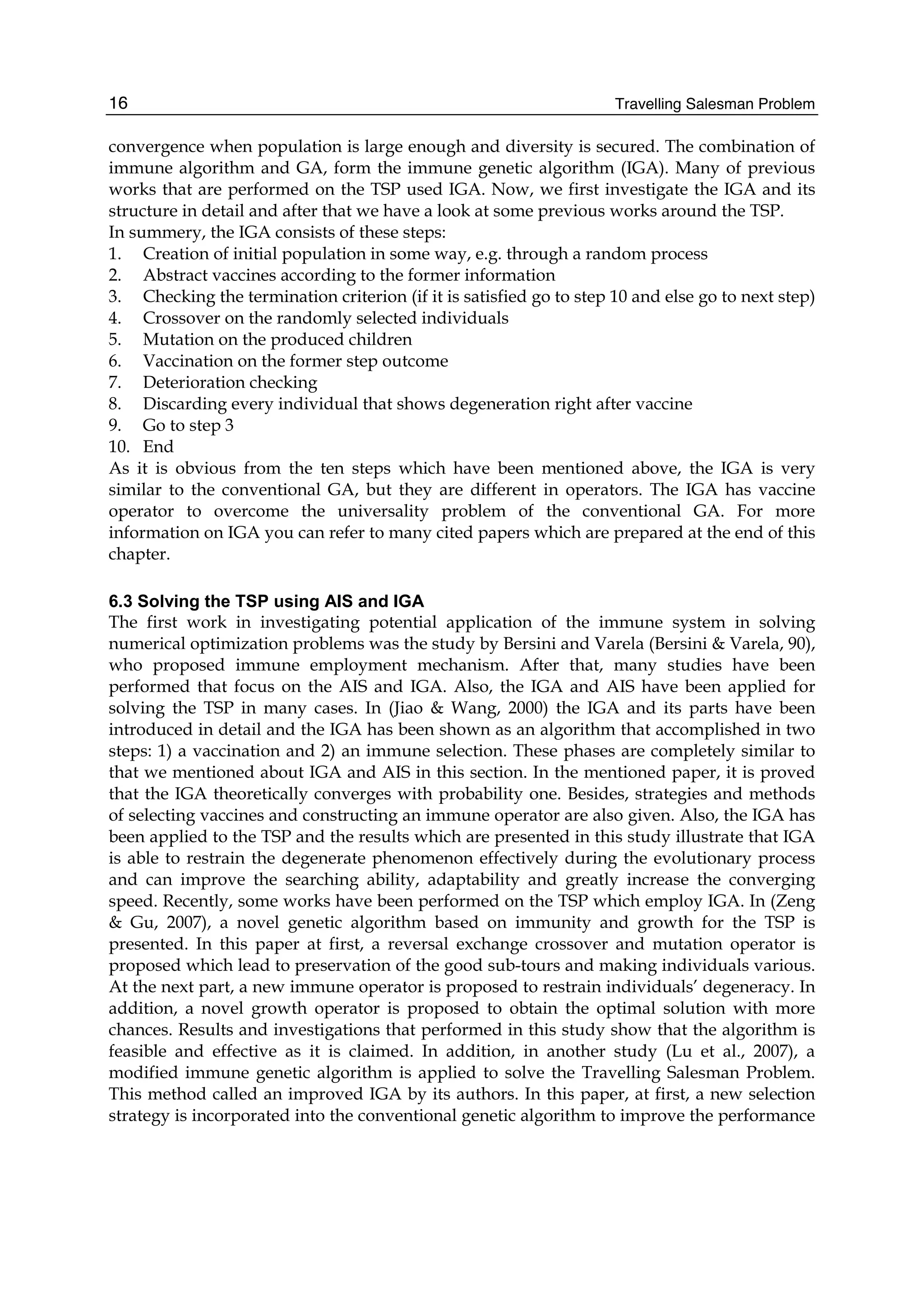


![Population-Based Optimization Algorithms for Solving the Travelling Salesman Problem 21
smaller tour length and also the greater number of bees. Based on these conditions the
authors prepare a relation as it is shown in equation 15, where:
θ
ρ, – Parameters given by the analyst,
)
,
( z
u
ξ
α – The normalized value of the partial route length
)
,
( z
u
ξ
β – The normalized value of the number of bees advertising the partial tour,
Y(u, z) – The set of partial tours that were visited by at least one bee.
z
u
z
u
Y
z
u
Y
z
u
z
u
e
z
u
z
u
e
z
u
p ,
),
,
(
)
,
(
)
,
(
)
,
(
)
,
(
)
,
(
)
,
( ∀
∈
∑
∈
−
−
= ξ
τ
θατ
ρβτ
ξ
θα
ξ
ρβ
ξ (15)
As it is shown in the mentioned work (Lucic Teodorovic, 2002), this bee system has been
tested on a large number of well known test benches such as Eil51.tsp, Berlin52.tsp, St70.tsp,
Pr76.tsp, Kroa100.tsp, Eil101.tsp, Tsp225.tsp and A280.tsp. Also, for improving the results in
each step, the 2-opt or 3-opt algorithms have been applied. The results reveal that the
mentioned method is very efficient. In all instances with less than 100 nodes, the bee system
achieves the optimal solution and in the large cases it has a significant improvement in
comparison to the other prevalent methods. The simulation results have been organized in
section nine.
One of the recent work for solving the TSP using bee’s behaviour and BCO algorithm is
(Teodorovic et al., 2006). In this paper the authors propose the Bee Colony Optimization
Metaheuristic (BCO). Moreover, this study, describes two BCO algorithms that the authors
call them, the Bee System (BS) and the Fuzzy Bee System (FBS). In the case of FBS the agents
(artificial bees) use approximate reasoning and rules of fuzzy logic in their communication
and acting. In this way, the FBS is capable to solve deterministic combinatorial problems, as
well as combinatorial problems characterized by uncertainty. In this paper, The BCO as a
new computational paradigm is described in detail at first. After that the TSP as a case study
has been solved using the proposed bee system. The proposed bee system is similar to that
had been seen in the previous investigated study but in this paper the BCO algorithm has
been described completely. For further information about the BCO algorithm please refer to
the related resources prepared at the end of the chapter.
8. Electromagnetism
8.1 Introduction
The Electromagnetism-like mechanism is a heuristic that was introduced by (Birbil Fang,
2003). The method utilizes an attraction-repulsion mechanism to move the sample points
towards the optimality. In other words, EM simulates the attraction-repulsion mechanism of
electromagnetism theory which is based on Coulomb’s law. The main concentration of the
first introduction of this heuristic was on the problems with bounded variables on the form
equal to equation 16.
Min(f(x)) s.t. x ∈[l,u] (16)](https://image.slidesharecdn.com/1270334-250526101849-18d8dedc/75/Traveling-Salesman-Problem-Federico-Greco-35-2048.jpg)
![Travelling Salesman Problem
22
where l and u are defined as the following form (equation 17):
[ , ] { , 1,... }
n k k k
l u x x l x u k n
= ∈ = (17)
-4
-2
0
2
4
-4
-2
0
2
4
-60
-40
-20
0
20
40
60
80
100
Fig. 6. A continuous optimization problem space
As an example, figure 6 illustrates continues problem space with l1=-60, l2=-4, l3=-4,
u1=+100, u2=+4 and u3=+4. The aim is to find the minimum value of the shown surface.
In stochastic global optimization, population based algorithms start with sample points
from feasible regions which are randomly selected. The regions of attraction are determined
according to objective function values and then a mechanism is invoked for exploration of
these candidate regions. The Genetic Algorithm is an example of this mechanism that
corresponds to the crossover, reproduction and mutation operators (Michalewicz, 1994).
Similarly, Birbil et al. construct a mechanism that encourages the points to converge to the
highly attractive valleys, and contrarily, discourages the points to move further away from
steeper hills. This is similar to the charge of particles in elementary electromagnetism. In this
approach, the charge of each point relates to the objective function value, which we are
trying to optimize and also determines the magnitude of attraction or repulsion of the point
over the sample population.
In addition, the combination force is exerted on the point via other points for finding a
direction for each point to move in subsequence iterations. Like the electromagnetic forces,
this force is calculated by adding vectorially the forces from each of the other points
calculated separately.
Finally, similar to the hybrid population-based algorithms (Glover Laguna, 1995), we may
apply a local search procedure to improve some of the objective function values observed in
the population.
Consider a problem in the form of (16) and the following parameters are given:
n dimension of the problem.
uk upper bound in the kth dimension.
lk lower bound in the kth dimension.
f (x) pointer to the function that is minimized.
For solving such problem using Electromagnetism-Like method, the following algorithm is
introduced by Birbil et al.](https://image.slidesharecdn.com/1270334-250526101849-18d8dedc/75/Traveling-Salesman-Problem-Federico-Greco-36-2048.jpg)
![Population-Based Optimization Algorithms for Solving the Travelling Salesman Problem 23
ALGORITHM 1. EM (m, MAXITER, LSIT ER, δ)
m: number of sample points
MAXITER: maximum number of iterations
LSIT ER: maximum number of local search iterations
δ: local search parameter, δ ∈ [0, 1]
1: Initialize ()
2: iteration ←1
3: while iteration MAXITER do
4: Local (LSIT ER, δ)
5: F ←CalcF ()
6: Move (F)
7: iteration ←iteration + 1
8: end while
The algorithm consists of four phases. The first phase is the initialization which determines the
initial position of the particles, second is the local search which gathers the local information of
each particle to improve it to its best local position, third is about calculating the force of each
particle and finally moves the particles. These phases are described in more details as follows.
8.2 Initialization
The initialization procedure is used to determine the place of the m particles (size of
population) at first iteration in an n dimensional feasible space. The distribution of the
particles is uniform between the lower bound and upper bound of the corresponding
variable. f(x) is the objective function and xbest is the particle which has the best value of f(x).
The initialization algorithm is as follow:
ALGORITHM 2. Initialize ()
1: for i = 1 to m do
2: for k = 1 to n do
3: λ ← U (0,1)
4: ( )
i
k k k k
x l u l
λ
← + −
5: end for
6: Calculate f (xi )
7: end for
8: xbest ← argmin{f (xi ), ∀i}
8.3 Local search
The local search procedure is used for gathering local information about xi and replacing the
particle with its best potential in its neighbour. The invoked local search by Birbil et al.,
works as follows: for each particle, in each dimension select a random step length and move
the ith particle along the direction. If the attained point has the better objective value than the
xi, the xi will be replaced by this point.
In this part of algorithm, any local search algorithm can be used but the following algorithm
is introduced by Birbil et al.
This is a simple random line search algorithm applied coordinate by coordinate. This
procedure does not require any gradient information to perform the local search. Instead of
using other powerful local search methods (Solis Wets, 1981), we have utilized this
procedure because we wanted to show that even with this trivial method, the algorithm
shows promising convergence properties.](https://image.slidesharecdn.com/1270334-250526101849-18d8dedc/75/Traveling-Salesman-Problem-Federico-Greco-37-2048.jpg)


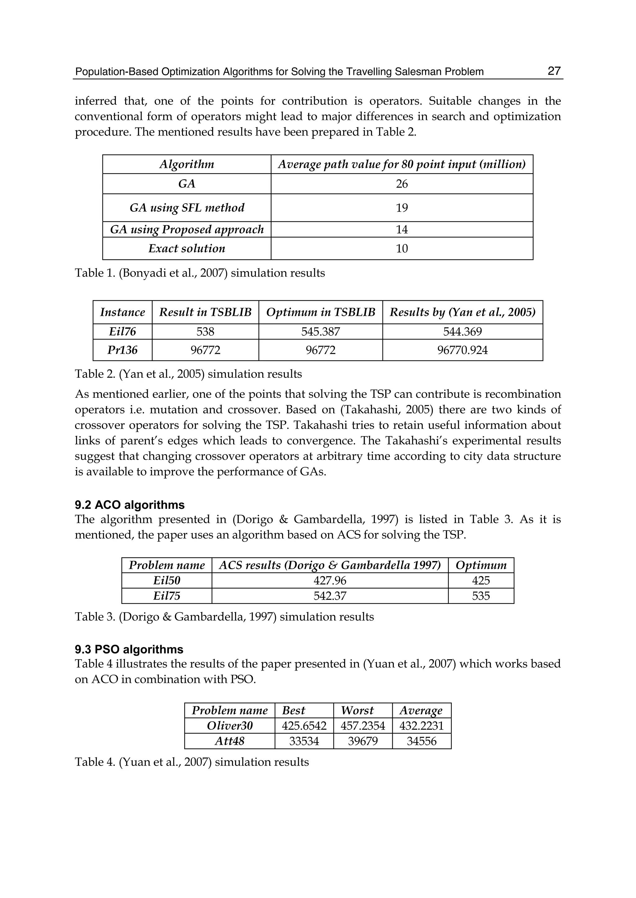

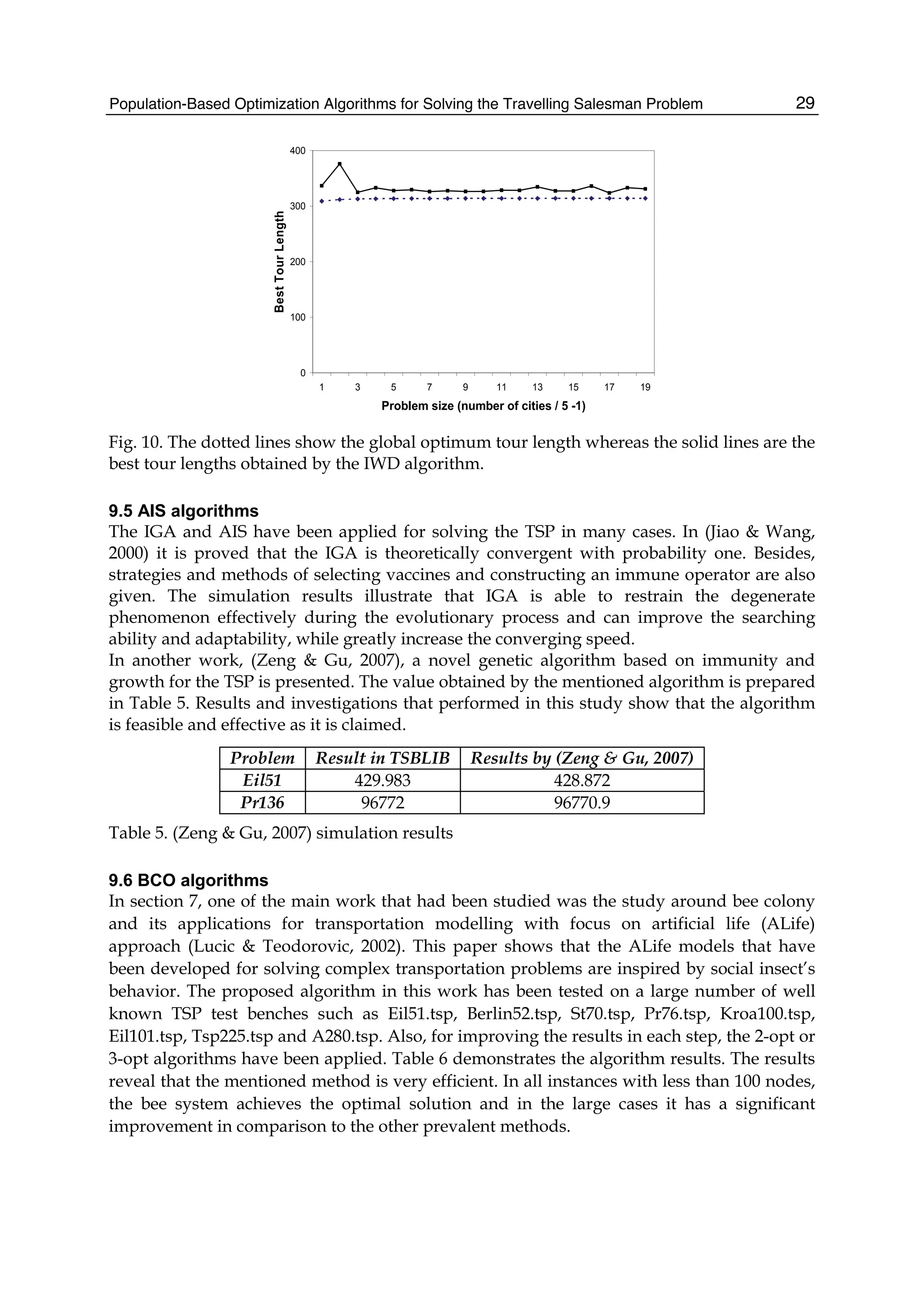


![2
Bio-inspired Algorithms for TSP and
Generalized TSP
Zhifeng Hao, Han Huang and Ruichu Cai
South China University of Technology
China
1. Introduction
The Traveling Salesman Problem (TSP) is to find a Hamiltonian tour of minimal length on a
fully connected graph. The TSP is a NP-Complete, and there is no polynomial algorithm to
find the optimal result. Many bio-inspired algorithms has been proposed to address this
problem. Generally, generic algorithm (GA), ant colony optimization (ACO) and particle
swarm optimization (PSO) are three typical bio-inspired algorithm for TSP. In this section
we will give a brief introduction to the above three bio-inspired algorithms and their
application to the TSP.
1.1 GAs for TSP
GAs were introduced by Holland in the 1970s [1]. These algorithms are adaptive search
techniques based on the mechanisms of natural selection and the survival of the fittest
concept of biological evolution. By simulating biological evolution, GAs can solve searching
problem domains effectively and easily apply to many of the current engineering problems.
GAs have been widely used in many applications of TSP and its extensions throughout the
literature [2-4].
A particularly nice introduction to GAs is given in Goldberg’s book [5]. The main idea
behind GAs is to start with randomly generating initial solutions and implements the
“survival of the fittest” strategy to increasing better solutions through generations. A
traditional GA process includes initial population generation, fitness evaluation,
chromosome selection, applying genetic operators for reproduction, and suspension
condition.
In designing a GA, how to encode a search solution is a primary and key issue [6]. Many
optimization operators for TSP were proposed by Goldberg [5]. A commonly used encoding
strategy is transposition expression [7]. In the transposition expression strategy, each city of
the TSP is encoded as a gene of the chromosome with the constraint that each city appears
once and only once in the chromosome. Transposition expression is the most nature
expression for TSP which based on the order of tour. While such method may leads to
infeasible tour after traditional crossover operator [7]. This is a common occurrence for TSP.
Although feasibility can be maintained in many ways named ‘repair algorithms’, such
algorithms can consume a considerable amount of time and can inhibit convergence.](https://image.slidesharecdn.com/1270334-250526101849-18d8dedc/75/Traveling-Salesman-Problem-Federico-Greco-49-2048.jpg)
![Travelling Salesman Problem
36
3 2 1 5 4 6 8 7
Figure 1. Transposition expression encoding method for TSP
Another typical encoding method is Random Keys encoding [8] which is introduced by
Bean. In Random Keys encoding a random numbers encode the structure of the solution.
Such representation ensures that feasible tours are maintained during the application of
genetic operators.
In the GA, the crossover and mutation are two of most important method for the success of
the algorithm. A crossover operator generates new individuals through recombining the
current population hopefully to retain good features from the parents. Numbers of different
crossovers have been proposed in the literatures to solve the TSP using a GA. The partially
mapped crossover [5,11-12], linear order crossover [13] and order based crossover
[5,8,11,12,14] are the commonly used crossover strategy in the TSP context. Expect the
commonly used crossover strategy, many different crossover strategy are proposed for the
TSP problem, for example: sub-tour crossover[15,16], edge recombination [17-20], distance
preserving crossover [21-22], generic crossover [23], NGA [24], EAX [25-26], GSX [27-28],
heuristic based crossover [29-35].
A mutation operator is used to enhance the diversity and provide a chance to escape from
local optima. Many mutation operators were proposed such as inverse, insert, displace,
swap, hybrid mutation [34], and heuristic mutation. The former five are realized by small
alterations of genes. Heuristic mutation was proposed by Cheng and Gen [37-38], which
adopts a neighborhood strategy to improve the solution.
At present, the genetic algorithm to solve the TSP has been to promote large-scale TSP, as
well as a multiple TSP (MTSP) and generalized TSP. A lot of progress was made recently.
Arthur E. Carter and Cliff T. Ragsdale propose a new GA chromosome and related
operators for the MTSP [39]. H. D. Nguyen, et al described a hybrid GA based on a parallel
implementation of a multi population steady-state GA involving local search heuristics [40].
Samanlioglu et.al proposes a methodology uses a “target-vector approach” in which the
evaluation function is a weighted Tchebycheff metric with an ideal point for a symmetric
multi-objective traveling salesman problem [41-43].
1.2 Ant colony optimization (ACO) for TSP
Ant Colony Optimization (ACO), first proposed by M. Dorigo et al. [44-46], is a population-
based, general-purpose heuristic approach to combinational optimization problems. The
earliest ACO algorithm [44-45], Ant System (AS), was applied to the TSP (mainly because
the TSP is “a shortest path problem to which the ant colony metaphor is easily adapted and
that it is a didactic problem” [4]. After that, most improved ACO algorithms also used the
TSP as a test problem and the result is promising.
As the name suggests, ACO took inspiration from the foraging behavior of real ant colonies.
Ants deposit pheromone on the ground they cover while working, forming a pheromone
trail. Other ants tend to follow the pheromone trail. Consider an ant colony exploring the
paths between their nest to a food source. At the beginning, the ants choose paths randomly
in equal rate since there’s no pheromone on the paths help them make the decision. Suppose
that every ant walk in the same speed, shorter paths accumulate pheromone faster than
longer paths because ants on those paths return earlier. A moment later, the difference in the](https://image.slidesharecdn.com/1270334-250526101849-18d8dedc/75/Traveling-Salesman-Problem-Federico-Greco-50-2048.jpg)
![Bio-inspired Algorithms for TSP and Generalized TSP 37
amount of pheromone on the paths becomes sufficient large so that the ants’ decision are
influenced and more ants select the shorter paths. Experiments show that this behavior can
lead the ant colony to the shortest path.
Figure 2. an ant colony exploits the paths between S and T. (A) The two paths are selected
with the same probability at first. (B) Ant 2 choosing the lower path returns to S earlier.
Thus pheromone on the lower path rises faster. (C) Most ants walk on the lower path after a
minute.
Typical ant algorithms stimulate the above foraging behavior of ant colonies using a set of
agents (artificial ants) and an indirect communication mechanism employing (artificial)
pheromone. A simple framework may look like this:
Loop /* at this level each loop is called iteration */
Each ant is positioned on a starting node.
Loop /* at this level each loop is called a step */
Each ant applies a stochastic state transition rule to incrementally build a solution
Until all ants have built a complete solution
A pheromone updating rule is applied
Until End condition
The stochastic state transition rule and the pheromone updating rule are two factor to the
success of the ACO. And many strategies have been proposed for these two operators. The
Ant Colony System (ACS) [48-50] and MAX-MIN Ant System (MMAS) [51] are among the
most successful algorithms [52]. Recent researches focus most on extending the applications
of ACO algorithms to more challenge problems. There’re also some studies on the
convergence theory of ACO algorithms too [47, 53-58].
1.3 PSO for TSP
The particle swarm optimization (PSO) was originally presented by Kennedy and Eberhart
in 1995 [59]. It is an algorithm based stochastic optimization technique which inspired by
social behavior among individuals. In the PSO system, individuals (we call them particles)
move around a multidimensional search space. Each particle represents a potential solution
of the problem, and can remember the best position (so1ution) it has reached. All the
particles can share their information about the search space, so there is a global best
solution.
In each iteration, every particle adjusts its velocity i
v and position i
x according to the
following formulas:
1 1 , 2 2 ,
( ) ( )
i i i pbest i i gbest i
i i i
v v c r x x c r x x
x x v
= + ∗ ∗ − + ∗ ∗ −
= +
(1)](https://image.slidesharecdn.com/1270334-250526101849-18d8dedc/75/Traveling-Salesman-Problem-Federico-Greco-51-2048.jpg)
![Travelling Salesman Problem
38
Where w is inertia weight, 1
c and 2
c are acceleration coefficients, 1
r and 2
r are two
independent random values between 0 and 1. xi,pbest is the best solution this particle has
reached; xi,gbest is the global best solution of all the particles until now.
Due to the continuous characters of the position of particles in PSO, the standard encoding
scheme of PSO can not be directly adopted for TSP. Much work was published to avoid
such problem. Clerc adopted discrete particle swarm optimization (DPSO)[60] to make PSO
suitable for solving TSP. Bo Liu, et al. proposes a PSO-based MA [61](PSOMA) for TSP,
which combined evolutionary searching mechanism of PSO and adaptive local search.
Yong-Qin Tao, et al. proposed a GRPSAC algorithm [62] combined ACO with PSO
organically and adds gene regulation operator at the same time, which make solution of TSP
problem more efficiency. Other recently work such as heuristic information method based
on improved fuzzy discrete PSO [63] and chaotic PSO algorithm [64] were proved to be
effective for TSP.
2. Ant colony optimization (ACO) for TSP
2.1 The method of ant colony optimization solving TSP
Among the bio-inspired algorithms, the ant colony optimization (ACO) is a popular
approach for TSP since it’s proposed by M.Dorigo in early nineties [65-66]. Ant colony
optimization (ACO) takes inspiration from the foraging behavior of some ant species. These
ants deposit pheromone on the ground in order to mark some favorable path that should be
followed by other ants of the colony. Ant colony optimization exploits a similar mechanism
for solving optimization problems.
In TSP, a set of cities is given and the distance between each of them is known. The goal is to
find a Hamiltonian tour of minimal length on a fully connected graph. This goal is very
similar with the ants to find the shortest path between the nest and the food source. In ant
colony optimization, the problem is tackled by simulating a number of artificial ants moving
on a graph that encodes the problem itself. A variable called pheromone is associated with
each edge and can be read and modified by ants. The artificial ants explore the pheromone
to find the most favorable path which is the shortest Hamiltonian Tour in TSP.
Ant colony optimization is an iterative algorithm. In an iterative step, each ant of the colony
builds a solution by walking from vertex to vertex on the graph with the constraint of not
visiting any vertex that has been visited before. The solution construction and the
pheromone updating are two main steps for the ACO. In the solution construction step, an
ant selects the next vertex to be visited according to a stochastic mechanism that is biased by
the pheromone. After the solution construction step, the pheromone is updated on the basis
of the quality of the solutions.
Under the above framework, many different version of the algorithm are proposed.
According to the M.Dorigo’s work [46,67], the Ant System (AS), MAX−MIN Ant System
(MMAS) and Ant Colony System (ACS) are three of most popular ant algorithms.
Following, we will give a short brief of those three algorithms on TSP.
2.1.1 Ant System (AS)
Ant System is the first ACO algorithm proposed in the literature [44,65-66]. Its main
characteristic is that, at each iteration, the pheromone values are updated by all the m ants
that have built a solution in the iteration itself. The pheromone ij, associated with the edge
joining cities i and j, is updated as follows:](https://image.slidesharecdn.com/1270334-250526101849-18d8dedc/75/Traveling-Salesman-Problem-Federico-Greco-52-2048.jpg)
![Bio-inspired Algorithms for TSP and Generalized TSP 39
1
(1 ) ij
m
k
ij ij
k
τ ρ τ τ
=
← − ⋅ + Δ
∑ (1)
where ρ is the evaporation rate, m is the number of ants, and
ij
k
τ
Δ is the quantity of
pheromone laid on edge (i, j) by ant k:
/ ( , ) ,
0 ,
ij
k
k
Q L if ant k used edge i j initstour
otherwise
τ
⎧
Δ = ⎨
⎩
(2)
where Q is a constant, and k
L is the length of the tour constructed by ant k.
In the construction of a solution, ants select the following city to be visited through a
stochastic mechanism. When ant k is in city i and has so far constructed the partial solution
Sp, the probability of going to city j is given by:
( )
[ ( )] [ ]
( )
[ ( )] [ ]
( )
0
gs gs
k
gr gr
gs
r J g
k
k
t
if s J g
t
P t
otherwise
α β
α β
τ η
τ η
∈
⎧
∈
⎪
⎪
= ⎨
⎪
⎪
⎩
∑ (3)
where ( )
k
J g is the set of cities not visited yet by ant k when at city g. The parameters α
and β control the relative importance of the pheromone versus the heuristic information ηij,
which is given by
1
ij
ij
d
η = , where ij
d is the distance between cities i and j.
2.1.2 MAX −MIN Ant System (MMAS)
The MAX −MIN Ant System [51] is an improvement over the original Ant System. In the
MMAS, only the best ant updates the pheromone trails and the value of the pheromone is
bound. The pheromone update is implemented as follows:
max max
min min
(1 ) ,
(1 ) ,
(1 ) ;
ij
ij
ij
best
ij
best
ij ij
best
ij
if
if
otherwise
τ ρ τ τ τ
τ τ ρ τ τ τ
ρ τ τ
⎧ − ⋅ + Δ
⎪
⎪
= − ⋅ + Δ
⎨
⎪
− ⋅ + Δ
⎪
⎩
(4)
where max
τ and min
τ min are respectively the upper and lower bounds imposed on the
pheromone and
ij
best
τ
Δ is:
1 ( , )
0 ;
ij
best
best
L if i j belongstothebest tour
otherwise
τ
⎧
Δ = ⎨
⎩
(5)](https://image.slidesharecdn.com/1270334-250526101849-18d8dedc/75/Traveling-Salesman-Problem-Federico-Greco-53-2048.jpg)
![Travelling Salesman Problem
40
where best
L is the length of the tour of the best ant.
For the max
τ and min
τ , they are typically obtained empirically and tuned on the specific
problem considered [68]. And some guidelines have been provided for defining min
τ and
max
τ on the basis of analytical considerations [51].
2.1.3 Ant Colony System (ACS)
The ACS was considered the most efficient algorithm on the TSP problem. The main
contribution of ACS [48, 50, 69] is introducing a novel local pheromone update in addition
to the global pheromone.
The local pheromone update is performed by all the ants after each construction step. Each
ant applies it only to the last edge traversed:
0
(1 )
ij ij
τ ϕ τ ϕ τ
= − ⋅ + ⋅ (6)
where ( ]
0,1
ϕ ∈ is the pheromone decay coefficient, and 0
τ is the initial value of the
pheromone.
Using the local update strategy, the pheromone concentration on the traversed edges is
decreased. So, the subsequent ants are encouraged to choose other edges and to produce
different solutions. This makes it less likely that several ants produce identical solutions
during one iteration.
2.2 An adaptive strategy for weight parameter
Many strategies for ACO have been studied, but little theoretical work has been done on
ACO’s parameters α and β, which control the relative weight of pheromone trail and
heuristic value. In this part, we will theoretical show the importance and functioning of α
and β. The theoretical analysis show that a fixed β may not enable ACO to use both heuristic
and pheromone information for solution when α = 1. An adaptive β strategy and a new
ACO called adaptive weight ant colony system (AWACS) with the adaptive β and α = 1 is
introduced. The numerical experiment results show that the AWACS is more effective and
steady than traditional ACS.
2.2.1 Theoretical analysis of the weight parameter
Given , ( )
k
a b J g
∈ , if ( ) ( )
k k
ga gb
P t P t
, which means that city a may be chosen by the ant
k as the next city to city g with higher probability than city b, then α and β satisfies the
following formula: ( ) ( ) [ ( )] [ ] [ ( )] [ ]
k k
ga gb ga ga gb gb
P t P t t t
α β α β
τ η τ η
⇔ .
When ( ) ( )
ga gb
t t
τ τ
= or ga gb
η η
= , for , 0
α β
∀ , the formula above holds, so we have:
( ) ( )
ga gb ga gb
k k
ga gb
ga gb ga gb
P t P t
η η τ τ
τ τ η η
=
⎧
⇔ ⎨
=
⎩
(8)](https://image.slidesharecdn.com/1270334-250526101849-18d8dedc/75/Traveling-Salesman-Problem-Federico-Greco-54-2048.jpg)


![This ebook is for the use of anyone anywhere in the United States
and most other parts of the world at no cost and with almost no
restrictions whatsoever. You may copy it, give it away or re-use it
under the terms of the Project Gutenberg License included with this
ebook or online at www.gutenberg.org. If you are not located in the
United States, you will have to check the laws of the country where
you are located before using this eBook.
Title: Il Regno d'Etruria
Author: vicomte de Eugène-Melchior Vogüé
Release date: July 9, 2013 [eBook #43174]
Most recently updated: October 23, 2024
Language: Italian
Credits: Produced by Carlo Traverso, Claudio Paganelli, Barbara
Magni and the Online Distributed Proofreading Team at
http://www.pgdp.net (This file was produced from images
generously made available by The Internet Archive)
*** START OF THE PROJECT GUTENBERG EBOOK IL REGNO
D'ETRURIA ***](https://image.slidesharecdn.com/1270334-250526101849-18d8dedc/75/Traveling-Salesman-Problem-Federico-Greco-60-2048.jpg)


![Championnet, l'Italia disingannata malediceva di nuovo i successori,
gl'imitatori di Carlo VIII e di Luigi XI.
Le memorie del generale Thiébault, pubblicate recentemente,
mostrano per qual naturale cammino la guerra difensiva diventò
guerra di conquista e per quale logica metamorfosi l'entusiasmo dei
liberatori si cambiò in spirito d'invasione e di rapina e quello dei
liberati in odio contro i nuovi oppressori. Si rabbrividisce a leggere le
scene di carneficina e di devastazione che l'inconsciente Thiébault
descrive allegramente, quando racconta l'occupazione di Napoli e
delle Calabrie. Ma più ancora di questi sanguinosi eccessi, la rapacità
dei vincitori esasperò gl'Italiani. Li spogliavano dei tesori d'arte, nei
quali la coscienza nazionale vedeva con ragione i veri emblemi della
patria smembrata, le più salde garanzie del diritto che essa aveva a
pretendere un destino pari all'altezza del suo genio. Paul-Louis
Courier testimone dell'esodo di questi dèi lari, già lo rimpiangeva
nelle sue eloquenti lamentazioni: “Tutto quel che apparteneva ai
Certosini, a Villa Albani, ai Farnese, agli Onesti, al Museo Clementino,
al Campidoglio, è portato via, saccheggiato, perduto o venduto.
Gl'Inglesi ne hanno avuto una gran parte, e alcuni commissari
francesi, sospettati di aver fatto cotesti traffici, son qui arrestati; ma
la cosa non avrà seguito. Una squadra di soldati, entrati nella
Biblioteca Vaticana, ha fra le altre rarità distrutto il famoso Terenzio
del Bembo, per prender le poche dorature onde il manoscritto era
ornato. La Venere di Villa Borghese è stata ferita in una mano da
qualche discendente di Diomede, e l'Ermafrodito, immane nefas!, ha
un piede rotto.„[1]
In Toscana, come a Roma e a Napoli, il triennio, gli anni di guerra
civile e straniera corsi tra il 1798 e il 1801, fu un'êra dolorosa di
disordini, di esazioni, di miseria per il popolo. Francesi, Napoletani,
Austro-Russi e insorti paesani opprimevano ugualmente i poveri
abitanti estenuati. Mai fu meglio appropriato il grido del poeta:
Ahi, serva Italia di dolore ostello,
Nave senza nocchiero in gran tempesta!](https://image.slidesharecdn.com/1270334-250526101849-18d8dedc/75/Traveling-Salesman-Problem-Federico-Greco-71-2048.jpg)