CHAPTER THREE:
TRANSPORTATION AND
ASSIGNMENT PROBLEM
2
Transportation Models
• Transportation model deals with a special class of linear
programming problem in which the objective is to
transport a homogenous commodity from various origins
or factories to different destinations or markets at a total
minimum cost.
• The purpose of this LP Model is to identify a distribution
plan that would minimize the cost of transporting
commodities from the origin (factory warehouses) to the
destination or the market (retail stores), taking into
account warehouse supplies and retail store demands as
well as transportation costs.
3
Transportation Problem
• Transportation problems deals with shipments from a number of
sources to a number of destinations.
• Typically each source is supply limited, each destination has
known demand and the shipment cost between sources and
destinations are given.
• The objective of such models is to determine how many units should
be shipped from each source /origin to each destination/market
so that total transportation costs are minimized.
4
Characteristics of transportation problems
1. A limited supply of commodity is available at certain sources
or origins such as factories.
2. There is a demand for the commodity at several destinations
such as warehouse, distribution centers, and retail stores
3. The quantity of supply at each source and the demand or
requirements at each destination is assumed to be constant.
4. The shipping (transportation ) costs per unit from each
source to each destination are assumed to be constant.
5
Characteristics of transportation problems
5. No shipments are allowed between sources or between
destinations and again all supply and demand quantities
are given in whole numbers (integers)
6. The problem is to determine how many units to ship
from each source to each destinations so that all demand
are satisfied at the minimum total shipping cost.
6
Assumptions
• A transportation LPM has the following assumptions
1. All goods be homogeneous, so that any origin is capable of
supplying any destination,
2. Transportation costs are a direct linear function of the
quantity shipped over any route
3. The total quantity available is equal to the total
demand required
7
Formulating transportation Model
• A transportation problem typically involves a set of sending
locations, which are referred to as origins, and a set of receiving
locations, which are referred to as destinations.
• In order to develop a model of a transportation problem, it is
necessary to have the following information :
1. Supply quantity (capacity) of each origin
2. Demand quantity of each destination
3. Unit transportation cost for each origin-destination route.
8
Overview of the transportation method
• The transportation method is similar in certain aspects to simplex
technique because both involve initial feasible solution that is
evaluated to determine if it can be improved
• More over, both involve displaying initial and improved solutions in a
series of tableaus/tables.
• Transportation method, however, requires considerably less
computational effort
• A solution to a transportation problem consists of quantities that are
assigned to the various routes (i.e. cells in the tables)
• The quantities (values) can range from zero, which implies that no
units will be shipped over that route, to a maximum that equals the
smaller of the two quantities: the row (supply) and column
(demand)
9
Example
Transportation table
To
From
Project
#1
Project
#2
Project
#3
Supply
Farm A C11 C12 C13 S1
Farm B C21 C22 C23 S2
Farm C C31 C32 C33 S3
Demand D1 D2 D3
10
Methods for Finding Initial Solution
There are three methods to develop initial feasible
solution
1. The Northwest-Corner method.
2. Least cost method (An intuitive approach)
3. Vogel’s Approximation Method
11
1. The Northwest-Corner method(NCM)
• The Northwest-Corner method is a systematic approach for developing an
initial feasible solution.
• Its chief advantages are that it is simple to use and easy to understand. Its chief
drawback is that it does not take transportation costs into account.
• The northwest corner method gets its name because the starting point for the
allocation process is the upper left-hand (Northwest) corner of the
transportation table.
• Example: For the ABC company problem, this would be the cell that
represents the route from Farm A to Project #1. The following set of principles
guides the allocation:
12
1. The Northwest-corner method(NCM)
1. Begin with the upper left-hand cell (Northwest-Corner), and
allocate as many units as possible to that cell. This will be the
smaller of the row supply and the column demand (Adjust
the row and column quantities to reflect the allocation).
2. Remain in a row or column until its supply or demand is
completely exhausted or satisfied, allocating the maximum
number of units to each cell in turn, until all supply has been
allocated (and all demand has been satisfied because we assume
total supply and demand are equal).
13
Example
ABC company has contracted to provide topsoil for three residential
housing developments. Topsoil can be supplied from three different
“farms” as follows:
Farm Weekly capacity (cubic yards)
A 100
B 200
C 200
Demand for the topsoil generated by the construction projects is:
Project Weekly demand(cubic yards)
1 50
2 150
3 300
14
Example
The manager of the ABC company has estimated the cost (in USD)
per cubic yard to ship over each of the possible routes:
Cost per cubic yard to
From Project #1 Project #2 Project #3
Farm A 4 2 8
Farm B 5 1 9
Farm C 7 6 3
Required: Solve the problem using a Northwest-Corner method
15
Solution
• The first step is to arrange the information into a
transportation table. This is shown in the following table:
To
From
Project
#1
Project
#2
Project
#3
Supply
Farm A 4 2 8 100
Farm B 5 1 9 200
Farm C 7 6 3 200
Demand 50 150 300 500
16
Initial Feasible Solution
To
From
Project #1 Project #2 Project #3 Supply
Farm A 4
50(first)
2
50(second)
8 100
Farm B 5 1
100(third)
9
100(fourth)
200
Farm C 7 6 3
200(last)
200
Demand 50 150 300 500
17
Solution
• The total cost is found by multiplying the quantities in
“completed” (i.e. non-empty) cells by the cell’s unit cost and,
then, summing those amounts. Thus:
• Total cost = 50(4) + 50(2) + 100(1) + 100(9) + 200(3) = $1900
18
2. Least Cost Method(LCM)
• This approach, also known as the Minimum-Cost Method, uses
lowest cell cost as the basis for selecting routes. The procedure is as
follows:
1. Identify the cell that has the lowest unit cost. If there is a tie,
select one arbitrarily. Allocate a quantity to this cell that is equal to
the lower of the available supply for the row and the demand for the
column.
2. Cross out the cells in the row or column that has been exhausted (or
both, if both have been exhausted), and adjust the remaining row or
column total accordingly.
3. Identify the cell with the lowest cost from the remaining cells.
Allocate a quantity to this cell that is equal to the lower of the
available supply of the row and the demand for the column.
4. Repeat steps (2) and (3) until all supply and demand have been
exhausted.
19
Example
ABC company has contracted to provide topsoil for three residential
housing developments. Topsoil can be supplied from three different
“farms” as follows:
Farm Weekly capacity (cubic yards)
A 100
B 200
C 200
Demand for the topsoil generated by the construction projects is:
Project Weekly demand(cubic yards)
1 50
2 150
3 300
20
Example
The manager of the ABC company has estimated the cost per cubic
yard (in USD) to ship over each of the possible routes:
Cost per cubic yard to
From Project #1 Project #2 Project #3
Farm A 4 2 8
Farm B 5 1 9
Farm C 7 6 3
Required: Solve the problem by least cost method
21
Solution
• The first step is to arrange the information into a transportation
table. This is shown in the following table:
To
From
Project
#1
Project
#2
Project
#3
Supply
Farm A 4 2 8 100
Farm B 5 1 9 200
Farm C 7 6 3 200
Demand 50 150 300 500
22
Solution
• Initial Feasible Solution for the ABC company using the
LCM
To
From
Project #1 Project #2 Project #3 Supply
Farm A 4
50
2 8
50
100
Farm B 5 1
150
9
50
200
Farm C 7 6 3
200
200
Demand 50 150 300 500
23
Solution
Therefore :
• Total cost = 50(4) + 50(8) + 150(1) + 50(9) + 200(3) = $1800
24
3. Vogel’sApproximation Method (VAM)
• The third method for determining an initial solution is based on the concept
of penalty cost or regret.
• If a decision maker incorrectly chooses from several alternative courses of
action, a penalty may be suffered (and the decision maker may regret the
decision that was made).
• VAM Method use the concept of opportunity cost (the penalty for not
taking the correct decision)
• In transportation problem, the courses of action are the alternative routes and
a wrong decision is allocating to a cell that does not contain the lowest cost.
25
3. Vogel’sApproximation Method (VAM)
• With VAM the basis of allocation is unit cost penalty
i.e. that column or row which has the highest
unit cost penalty (difference between the lowest
and the next highest cost) is selected first for
allocation and the subsequent allocations in cells are
also done keeping in view the highest unit cost penalty
26
Steps in VAM
Step 1: For each column and row, determine its penalty
cost by subtracting their two of their least cost .
Step 2: Select row/column that has the highest penalty
cost in step 1
Step 3:Assign as much as allocation to the selected
row/column that has the least cost
Step 4: Block those cells that cannot be further allocated
Step 5: Repeat above steps until all allocations have been
assigned
27
Example
From To A B C Supply
1 6 8 10 150
2 7 11 11 175
3 4 5 12 275
Demand 200 100 300 600
28
Solution
Step1: Determine the penalty cost
(8-6)
(11-7)
(5-4)
(6-4) (8-5) (11-10)
29
Solution
Highest penalty
cost
Step 2:
Step 3: assign the maximum allocation to the least cost
30
Solution
Step 4: 1st
Iteration
31
Solution
Step 5: Second Iteration
32
Solution
Step 6: Third Iteration
33
Solution
Therefore,
Total cost = (150x10)+(7x175) +(25x4)+(100x5)+(150x12)= $5,125
34
Evaluating a Solution for Optimality
• There are two optimality evaluation methods.
These are:
1. The Stepping-stone method
2. The MODI method
35
The Stepping-stone method
• The Stepping-stone method involves tracing a series of closed paths
in the transportation table, using one such path for each empty
cell.
• The path represents a shift of one unit into an empty cell, and it
enables the manager or analyst to answer a “what-if” question
• The stepping-stone path also can be used to determine the
maximum number of units that can be shifted into the empty cell, as
well as modifications to other completed cells needed to compensate for
the shift into the previously unused cell.
36
The Stepping-stone method
• Rules for tracing Stepping-stone paths:
1. All unoccupied cells must be evaluated. Evaluate cells one at a
time.
2. Except for the cell being evaluated, only add or subtract in
occupied cells. (It is permissible to skip over unoccupied cells to
find an occupied cell from which the path can continue.)
3. A path will consist of only horizontal and vertical moves,
starting and ending with the empty cell that is being evaluated.
4. Alter + and - signs, beginning with a + sign in the cell being
37
The Stepping-stone method
• The general implication of the plus and minus
signs is that cells with “+” signs mean one unit
would be added, cells with a “–” sign indicate
one unit would be subtracted.
The Stepping-stone method
38
Example: Let’s consider the following initial tableau from the
Min Cost algorithm
These are basic
variables
There are
Non-basic variables
The Stepping-stone method
39
+
- +
-
Add min value of all –ve cells into cell that has “+” sign, and subtracts the
same value to the “-ve” cells Thus, max –ve is min (200,25) = 25, and we
add 25 to cell A1 and B3, and subtract it from B1 and A3
Stepping stone
40
The above New tableau gives the min cost = 25*6 + 125*10 + 175*11
175*4 + 100* 5 = $4525
41
The Modified Distribution Method (MODI)
MODI (MOdified DIstribution) is a modified version of the
stepping-stone method in which mathematical equations replace
the stepping-stone paths.
- In the table, the extra left-hand column with the ui symbols and
the extra top row with the vj symbols represent values that must be
computed.
- Computed for all cells with allocations :
ui + vj = cij = unit transportation cost for cell ij
42
The Modified Distribution Method (MODI)
There are five steps for MODI Method:
1. Develop an initial solution.
2. Compute the ui and vj values for each row and column.
3. Compute the cost change, kij, for each empty cell.
4. Allocate as much as possible to the empty cell that will
result in the greatest net decrease in cost (most negative kij)
5. Repeat steps 2 through 4 until all kij values are positive or
zero
43
Example
• Initial feasible solution
• Total cost= (8*25)+(125*10)+(175*11)+(200*4)+(75*5)=4450
From TO A B C Supply
1 6 8
25
10
125
150
2 7 11 11
175
175
3 4
200
5
75
12 275
Demand 200 100 300 600
Solution
44
The Minimum Cell Cost Initial Solution
The Modified Distribution Method (MODI)
45
- Formulas for cells containing allocations:
x1B: u1 + vB = 8
x1C: u1 + vC = 10
x2C: u2 + vC = 11
x3A: u3 + vA = 4
x3B: u3 + vB = 5
We have five equations with 6 unknowns, therefore let u1 = 0 and solve to obtain:
vB = 8, vC = 10, u2 = 1, u3 = -3, vA= 7
The Initial Solution with All ui and vj Values
The Modified Distribution Method (MODI)
46
• Each MODI allocation replicates the stepping-stone allocation.
• Use following to evaluate all empty cells:
cij - ui - vj = kij
where kij equals the cost increase or decrease that would occur by allocating to a cell.
- For the empty cells in the table :
x1A: k1A = c1A - u1 - vA = 6 - 0 - 7 = -1
x2A: k2A = c2A - u2 - vA = 7 - 1 - 7 = -1
x2B: k2B = c2B - u2 - vB = 11- 1 - 8 = +2
x3C: k3C = c3C - u3 -vC = 12 - (-3) - 10 = +5
The Modified Distribution Method (MODI)
47
- After each allocation to an empty cell, the ui and vj values must be recomputed.
The Second Iteration of the MODI Solution Method
The Modified Distribution Method (MODI)
48
Recomputing ui and vj values:
x1A: u1 + vA = 6, vA = 6 x1C: u1 + vC = 10, vC = 10 x2C: u2 + vC = 11, u2 = 1
x3A: u3 + vA = 4, u3 = -2 x3B: u3 + vB = 5, vB = 7
The New ui and vj Values for the Second Iteration
The Modified Distribution Method (MODI)
49
- Cost changes for the empty cells, cij - ui - vj = kij;
x1B: k1B = c1B - u1 - vB = 8 - 0 - 7 = +1
x2A: k2A = c2A - u2 - vA = 7 - 1 - 6 = 0
x2B: k2B = c2B - u2 - vB = 11 - 1 -7 = +3
x3C: k2B = c2B - u3 - vC = 12 - (-2) - 10 = +4
- Since none of the values are negative, solution obtained is
optimal.
- Cell 2A with a zero cost change indicates a multiple optimal
solution. Therefore:
Total cost: (6*25)+(10*125)+(11*175)+(175*4)+(5*100)=4525
50
Special Issues
1. Alternate Optimal Solutions- Sometimes, transportation
problems have multiple optimal solutions. In such cases, it can be
useful for a manager to be aware of alternate solutions, because
this gives the manager an option of bringing non-quantitative
considerations into the decision.
2. Degeneracy- A solution is degenerate if the number of occupied
cells is less than the number of rows plus the number of columns
minus one. i.e., there are too few occupied cells to enable all the
empty cells to be evaluated (m+n-1 < number of occupied cell).
51
Special Issues
3. Unacceptable Routes-In some cases, an origin-destination
combination may be unacceptable. This may be due to weather
factors, equipment breakdowns, labor problems, or skill requirements
that either prohibit, or make undesirable, certain combinations
(routes).
4. Unequal Supply and Demand- if supply and demand are not
equal, it is necessary to modify the original problem so that supply
and demand are equal. This is accomplished by adding either a
dummy column or a dummy row ( with a zero cell costs).
52
ASSIGNMENT PROBLEMS
53
Assignment Problems
• The Assignment Problem is a special case of Transportation
Problem in which the number of sources and destinations are the
same, and the objective is to assign the given job (task) to most
appropriate machine (person) so as to optimize the objective like
minimizing cost.
• Assignment is a problem because people possess varying
abilities for performing different jobs and, therefore, the costs of
performing the jobs by different people are different.
• Obviously, if all persons could do a job in the same time or at the
same cost then it would not matter who of them is assigned the job.
• Example : Assignment of workers to machines, clerks to various
counters, salesmen to different sales areas, service crews to
different districts.
54
Characteristics of theAssignment Problem
1. The availability of resources are finite in numbers such as
availability of workers, machines, project managers, sales man,
jobs etc.
2. These availability of resources can be assigned only on one to one
basis. i.e job can be assigned to particular employee only once.
3. The outcome (result) are expressed in terms of cost, time or
profit
4. The assignment methods aim at either cost minimization or
profit maximization.
5. For one to one assignment, the problem has to be of the balanced
type, otherwise it has to be converted into a balanced problem or
in to square matrix.
55
Presentation of the assignment problem
• The problem can be presented by the following tables:
Cost or time taken by workers on various job is indicated in matrix
cells as Cij
Workers Jobs
A B C D
1 C1a C1b C1c C1d
2 C2a C2b C2c C2d
3 C3a C3b C3c C3d
4 C4a C4b C4c C4d
56
HungarianAssignment method (HAM)
There are 6 steps :
Step 1. Locate the smallest cost element in each row of
the cost matrix. Then, subtract this smallest from
each element in that row. As a result, there shall be at
least one zero in each row of this new matrix.
Step 2. Now consider each column of the reduced cost
matrix from step 1 and locate smallest element in it.
Subtract the smallest value from each element of
the column . There would , again be at least one zero in
each column of the second reduced cost matrix.
57
HungarianAssignment method (HAM)
Step 3: Draw the minimum number of horizontal and vertical lines
to cover all zero elements. If the number of lines drawn is equal
to the number of rows/columns (n) the solution is optimal,
and proceeds to step 6. If the number of lines drawn is smaller than
n, go to step 4.
Step 4. Select the smallest uncovered cost element of the modified
matrix from step 3. Subtract this element from all uncovered
elements including itself and add this element to each value located
at the intersection of any lines.
Step 5: Repeat steps 3 and 4 until an optimal solution is obtained.
Step 6: Make feasible job assignments on zero elements .
58
Example
• Assign workers 1,2,3,4 to jobs A,B,C,D. Time taken by workers
from different jobs are given in the matrix.
Workers Jobs
A B C D
1 45 40 51 67
2 55 40 61 53
3 49 52 48 64
4 41 45 60 55
59
Solution
Step 1: Row minima's have been identified. These values are to
be subtracted from all values of the respective rows
Workers Jobs Row
minima
A B C D
1 45 40 51 67 40
2 55 40 61 53 40
3 49 52 48 64 48
4 41 45 60 55 41
60
Solution
Reduced time matrix is obtained thus ( revised time matrix I)
Workers jobs
A B C D
1 5 0 11 27
2 15 0 21 13
3 1 4 0 16
4 0 4 19 14
Column minima 0 0 0 13
61
Solution
Step 2: Now we obtain minimum values of each column from the
above reduced time matrix I and subtract these from each
respective column elements to achieve revised matrix II
Workers Jobs
A B C D
1 5 0 11 14
2 15 0 21 0
3 1 4 0 3
4 0 4 19 1
62
Solution
Step 3: Now drawing minimum number of horizontal/ vertical
lines to cover all zero elements we get matrix III below
Workers Jobs
A B C D
1 5 0 11 14
2 15 0 21 0
3 1 4 0 3
4 0 4 19 1
63
Solution
• Since, the number of lines drawn is 4=n, the solution is
optimal. So, proceed step 6
Step 6: making assignments on zero elements , we obtain
Hence, jobs have been assigned on zero elements 4A,1B,3C,2D
Total time=41+40+48+53=182 min(optimal)
Workers Jobs
A B C D
1 5 0 11 14
2 15 0 21 0
3 1 4 0 3
4 0 4 19 1
64
Special Cases in Assignment Problems
 Certain situations can arise in which the model deviates slightly from
that previously described. Among those situations are the following:
1. The number of rows does not equal the number of columns (Unbalanced
Assignment Problems)
2. Certain matches are undesirable or not allowed (Prohibited
Assignment Problems)
3. The problem involves maximization rather than minimization
(Maximization Assignment Problem)…(Reading Assignment)… get
opportunity loss table and follow the same procedure.
4. Multiple solution exist
65
Thank you

Ch 3.pptx
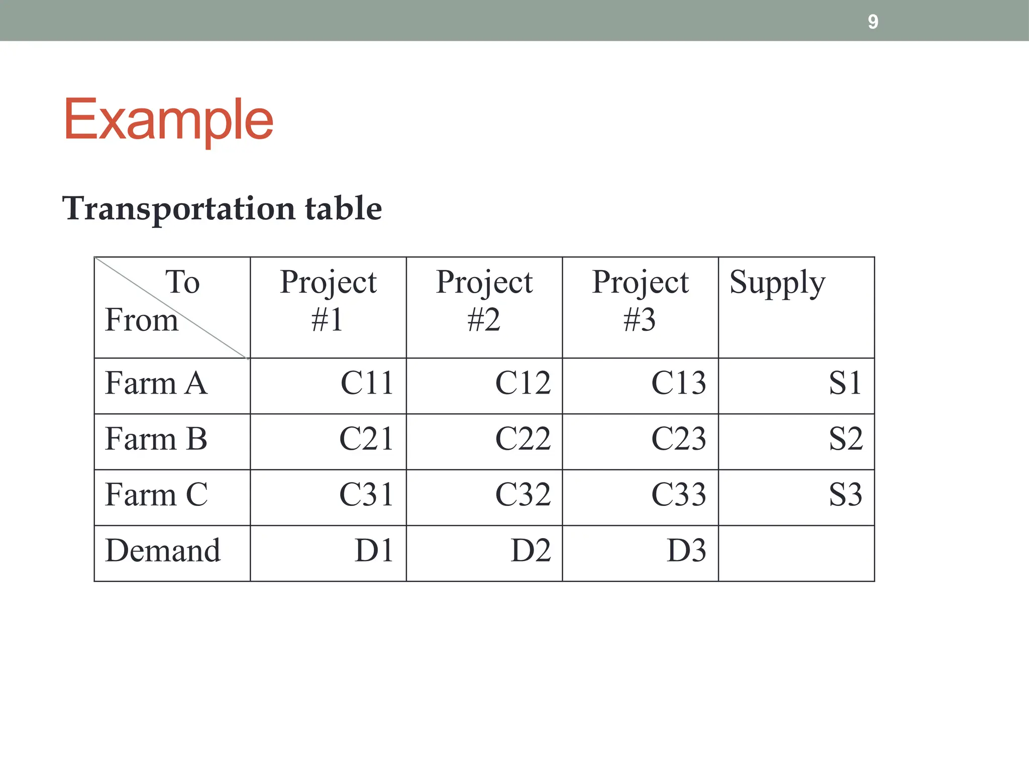
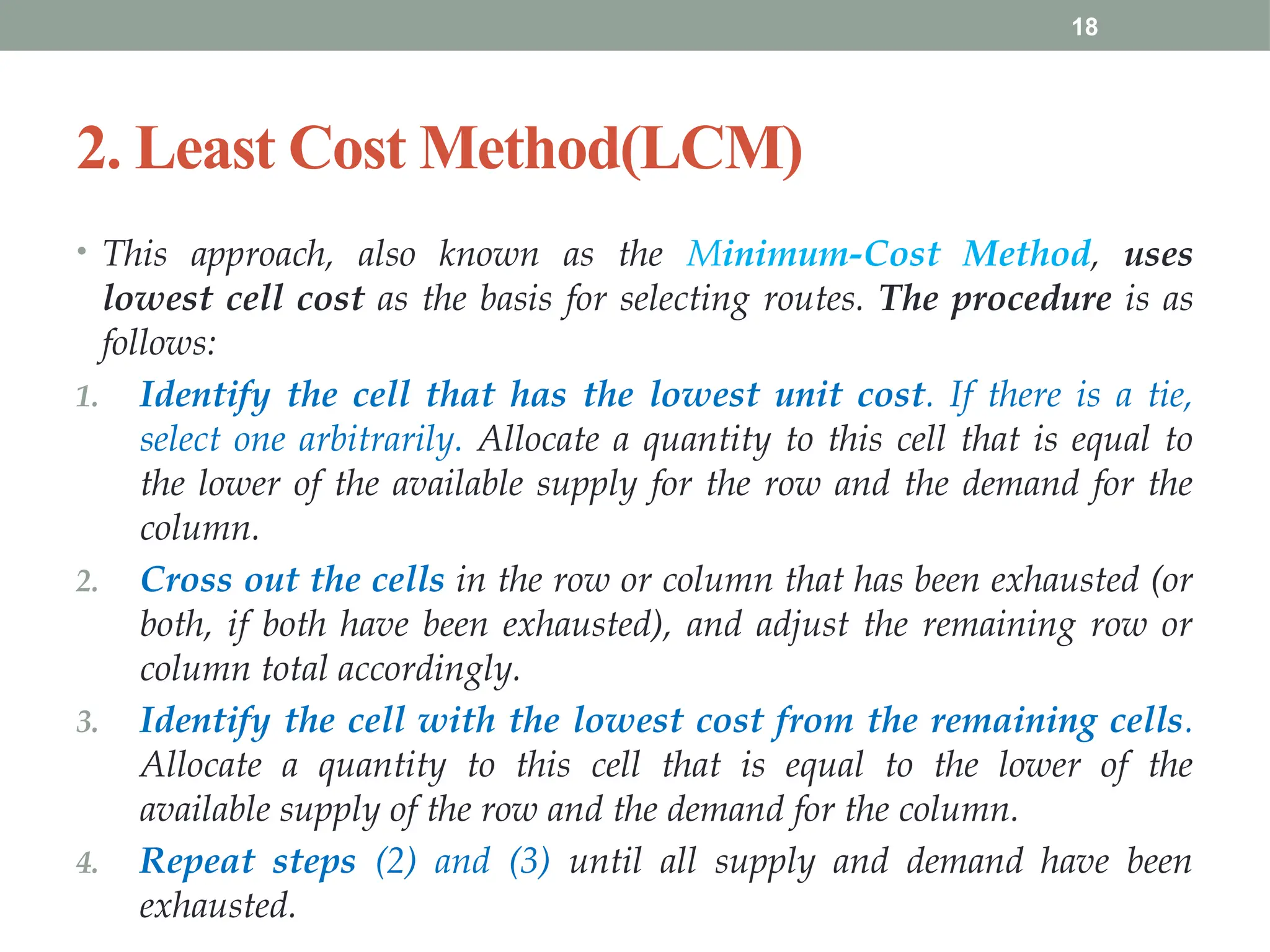
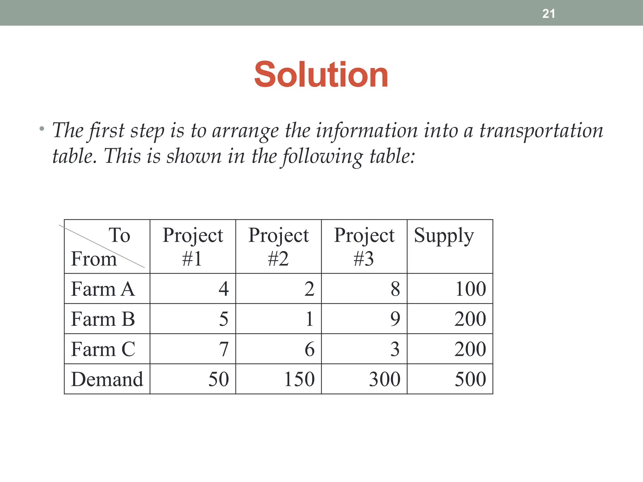
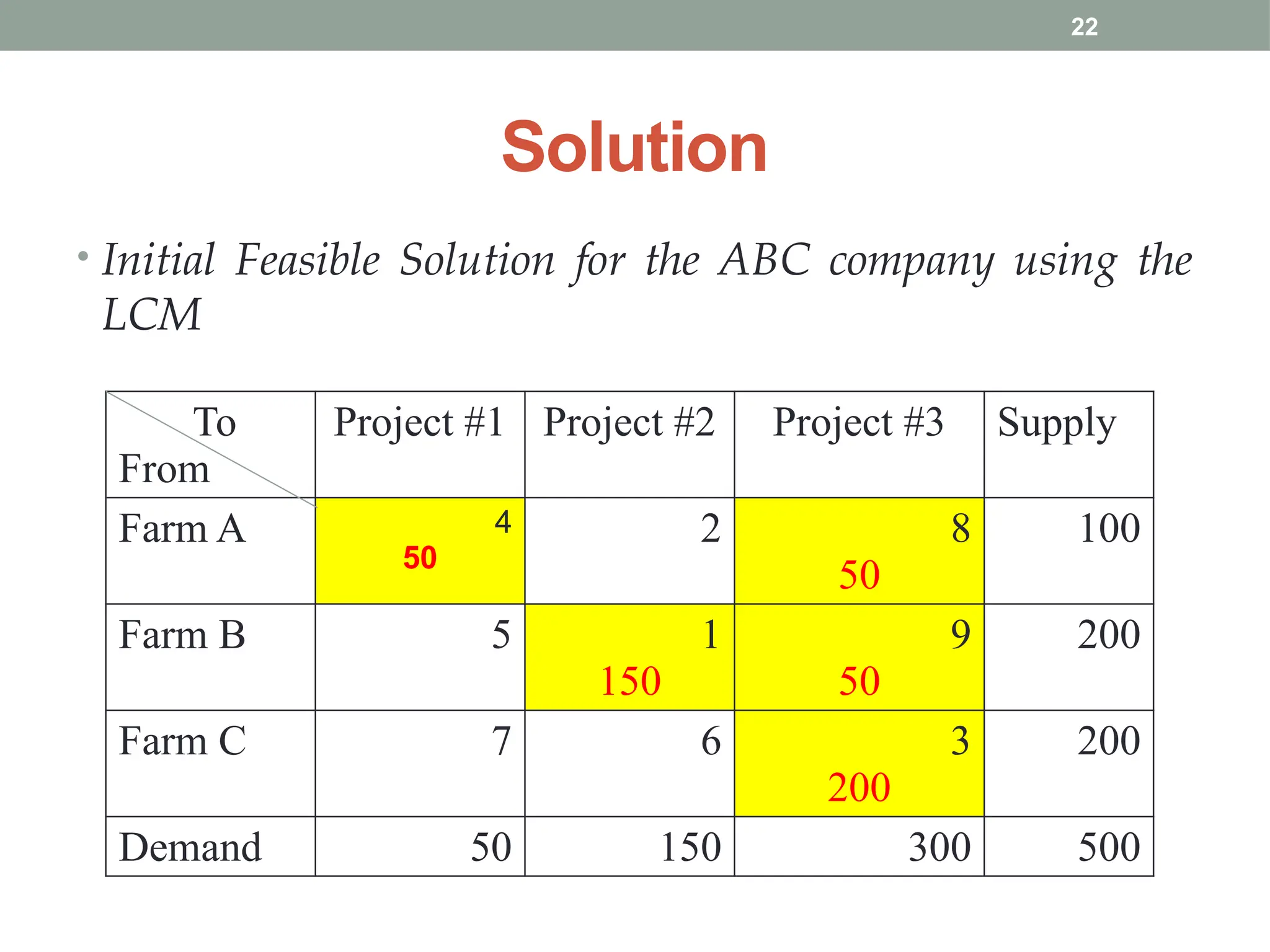
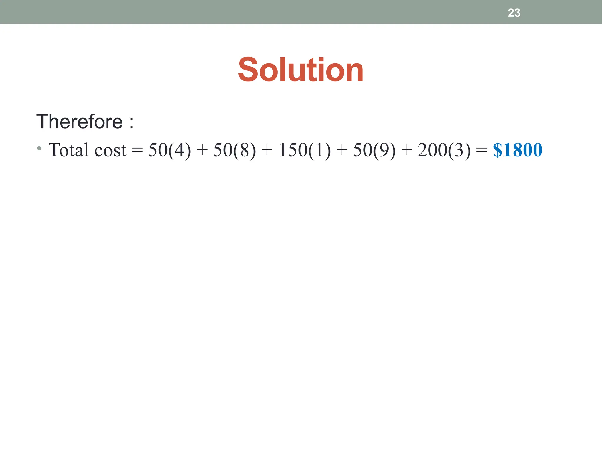
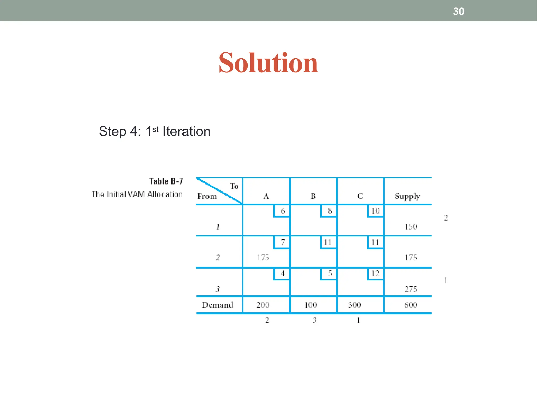
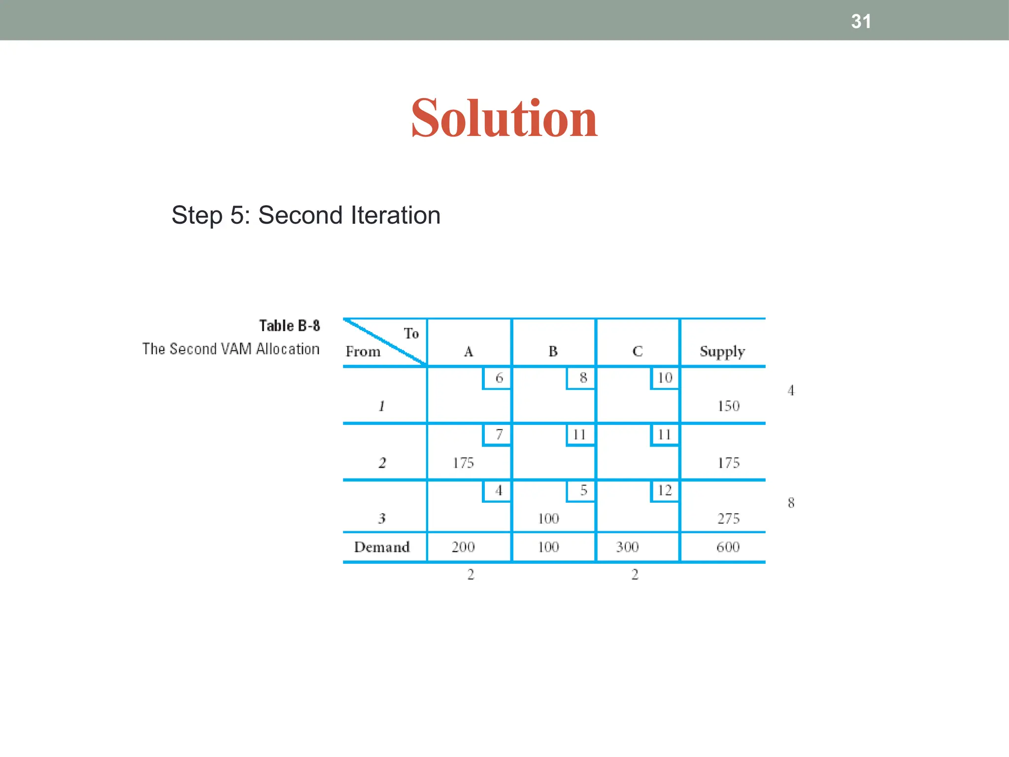
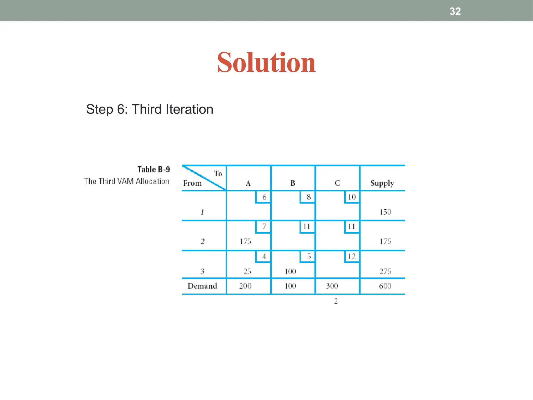
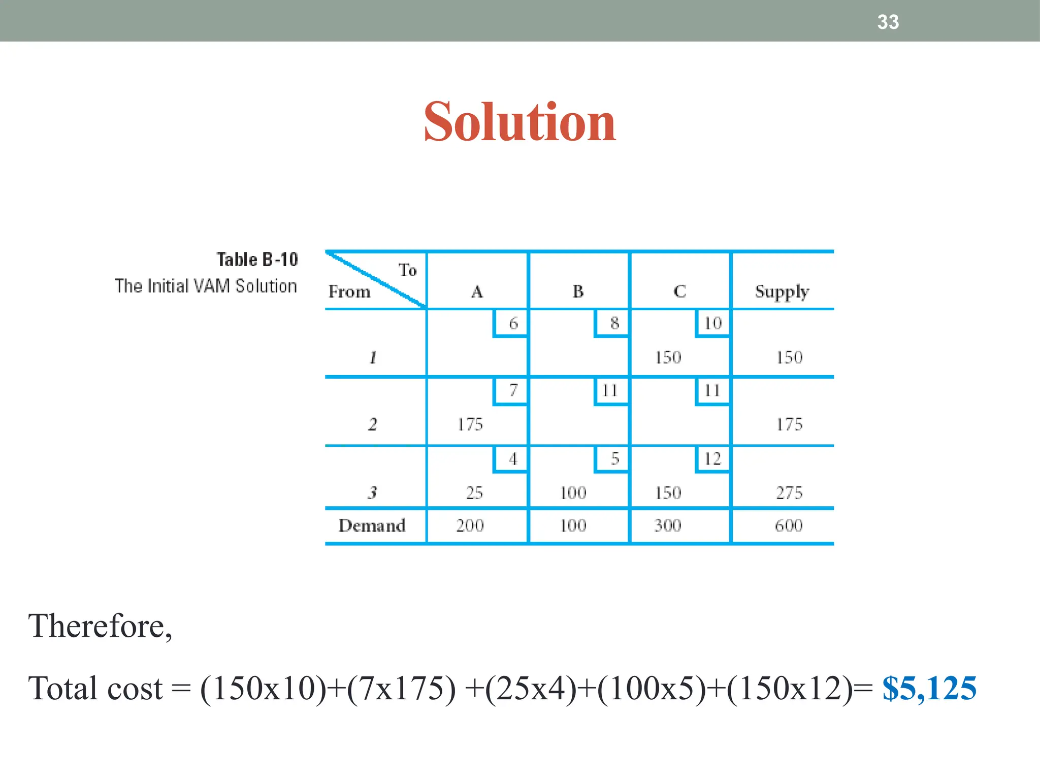
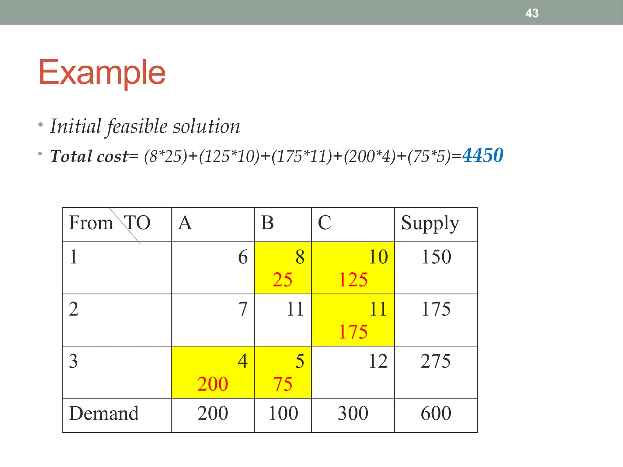
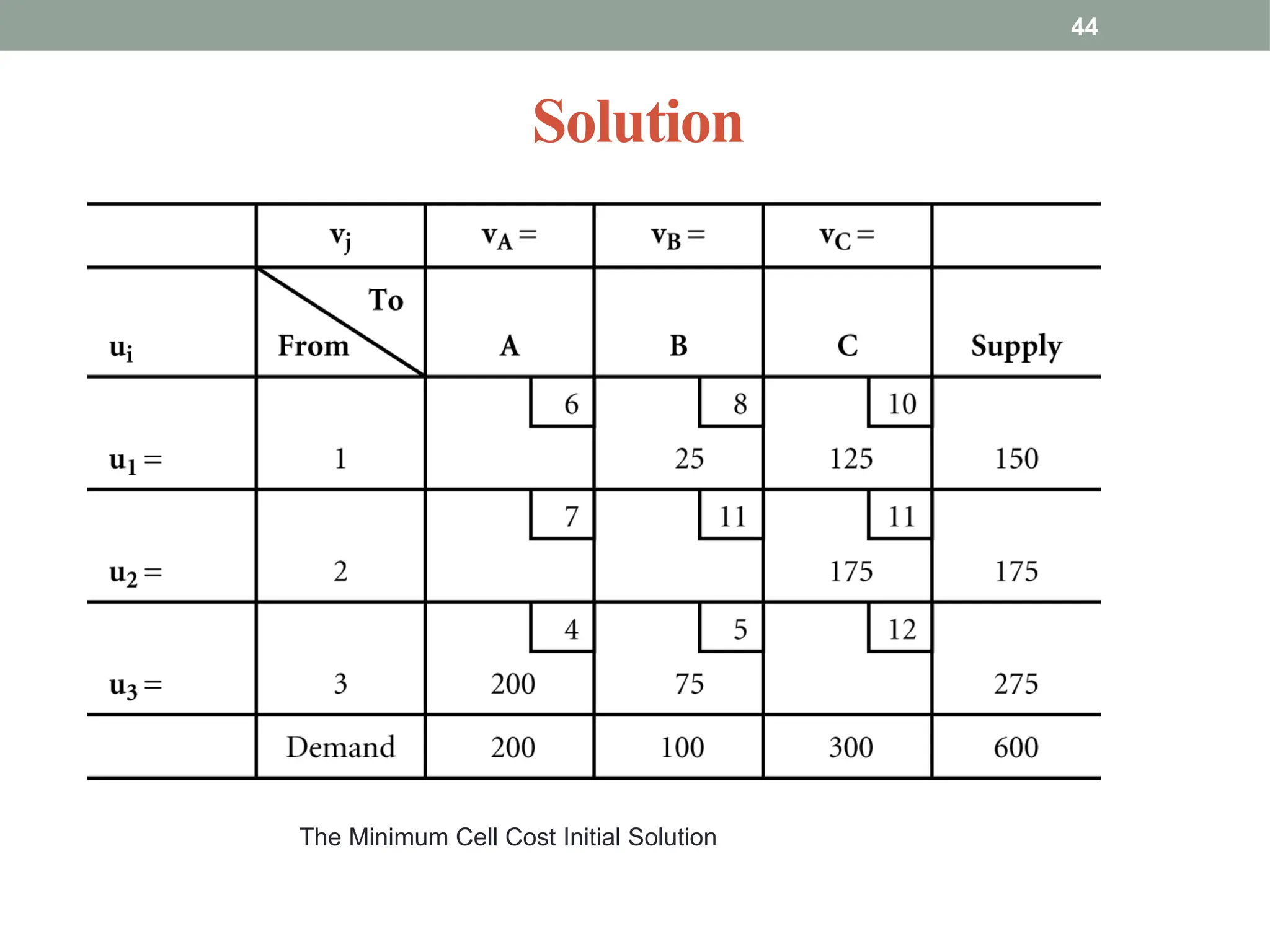
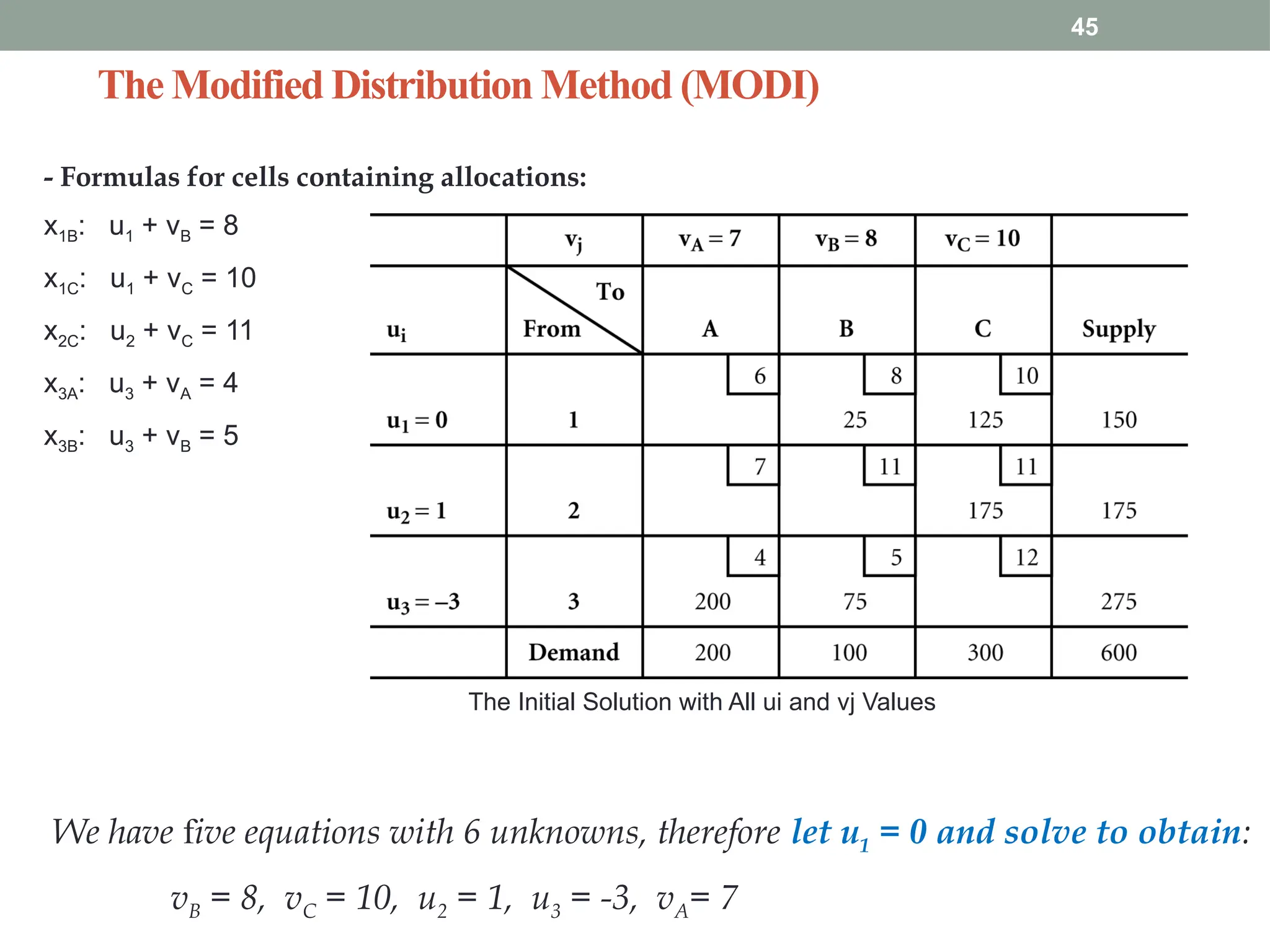
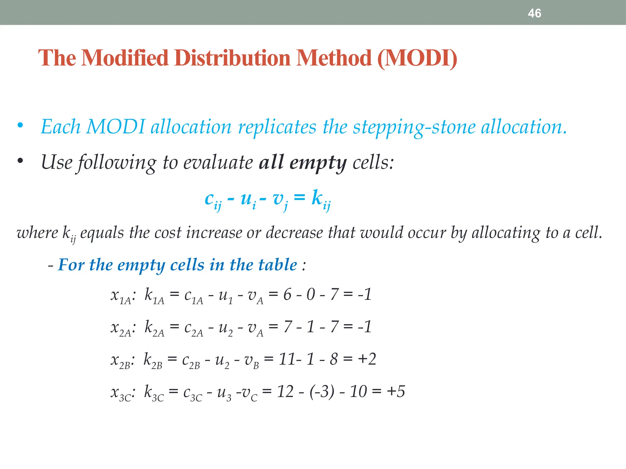
Transportation and Assignment Problems are special types of linear programming problems used in operations research.

  • 1.
  • 2.
    2 Transportation Models • Transportationmodel deals with a special class of linear programming problem in which the objective is to transport a homogenous commodity from various origins or factories to different destinations or markets at a total minimum cost. • The purpose of this LP Model is to identify a distribution plan that would minimize the cost of transporting commodities from the origin (factory warehouses) to the destination or the market (retail stores), taking into account warehouse supplies and retail store demands as well as transportation costs.
  • 3.
    3 Transportation Problem • Transportationproblems deals with shipments from a number of sources to a number of destinations. • Typically each source is supply limited, each destination has known demand and the shipment cost between sources and destinations are given. • The objective of such models is to determine how many units should be shipped from each source /origin to each destination/market so that total transportation costs are minimized.
  • 4.
    4 Characteristics of transportationproblems 1. A limited supply of commodity is available at certain sources or origins such as factories. 2. There is a demand for the commodity at several destinations such as warehouse, distribution centers, and retail stores 3. The quantity of supply at each source and the demand or requirements at each destination is assumed to be constant. 4. The shipping (transportation ) costs per unit from each source to each destination are assumed to be constant.
  • 5.
    5 Characteristics of transportationproblems 5. No shipments are allowed between sources or between destinations and again all supply and demand quantities are given in whole numbers (integers) 6. The problem is to determine how many units to ship from each source to each destinations so that all demand are satisfied at the minimum total shipping cost.
  • 6.
    6 Assumptions • A transportationLPM has the following assumptions 1. All goods be homogeneous, so that any origin is capable of supplying any destination, 2. Transportation costs are a direct linear function of the quantity shipped over any route 3. The total quantity available is equal to the total demand required
  • 7.
    7 Formulating transportation Model •A transportation problem typically involves a set of sending locations, which are referred to as origins, and a set of receiving locations, which are referred to as destinations. • In order to develop a model of a transportation problem, it is necessary to have the following information : 1. Supply quantity (capacity) of each origin 2. Demand quantity of each destination 3. Unit transportation cost for each origin-destination route.
  • 8.
    8 Overview of thetransportation method • The transportation method is similar in certain aspects to simplex technique because both involve initial feasible solution that is evaluated to determine if it can be improved • More over, both involve displaying initial and improved solutions in a series of tableaus/tables. • Transportation method, however, requires considerably less computational effort • A solution to a transportation problem consists of quantities that are assigned to the various routes (i.e. cells in the tables) • The quantities (values) can range from zero, which implies that no units will be shipped over that route, to a maximum that equals the smaller of the two quantities: the row (supply) and column (demand)
  • 9.
    9 Example Transportation table To From Project #1 Project #2 Project #3 Supply Farm AC11 C12 C13 S1 Farm B C21 C22 C23 S2 Farm C C31 C32 C33 S3 Demand D1 D2 D3
  • 10.
    10 Methods for FindingInitial Solution There are three methods to develop initial feasible solution 1. The Northwest-Corner method. 2. Least cost method (An intuitive approach) 3. Vogel’s Approximation Method
  • 11.
    11 1. The Northwest-Cornermethod(NCM) • The Northwest-Corner method is a systematic approach for developing an initial feasible solution. • Its chief advantages are that it is simple to use and easy to understand. Its chief drawback is that it does not take transportation costs into account. • The northwest corner method gets its name because the starting point for the allocation process is the upper left-hand (Northwest) corner of the transportation table. • Example: For the ABC company problem, this would be the cell that represents the route from Farm A to Project #1. The following set of principles guides the allocation:
  • 12.
    12 1. The Northwest-cornermethod(NCM) 1. Begin with the upper left-hand cell (Northwest-Corner), and allocate as many units as possible to that cell. This will be the smaller of the row supply and the column demand (Adjust the row and column quantities to reflect the allocation). 2. Remain in a row or column until its supply or demand is completely exhausted or satisfied, allocating the maximum number of units to each cell in turn, until all supply has been allocated (and all demand has been satisfied because we assume total supply and demand are equal).
  • 13.
    13 Example ABC company hascontracted to provide topsoil for three residential housing developments. Topsoil can be supplied from three different “farms” as follows: Farm Weekly capacity (cubic yards) A 100 B 200 C 200 Demand for the topsoil generated by the construction projects is: Project Weekly demand(cubic yards) 1 50 2 150 3 300
  • 14.
    14 Example The manager ofthe ABC company has estimated the cost (in USD) per cubic yard to ship over each of the possible routes: Cost per cubic yard to From Project #1 Project #2 Project #3 Farm A 4 2 8 Farm B 5 1 9 Farm C 7 6 3 Required: Solve the problem using a Northwest-Corner method
  • 15.
    15 Solution • The firststep is to arrange the information into a transportation table. This is shown in the following table: To From Project #1 Project #2 Project #3 Supply Farm A 4 2 8 100 Farm B 5 1 9 200 Farm C 7 6 3 200 Demand 50 150 300 500
  • 16.
    16 Initial Feasible Solution To From Project#1 Project #2 Project #3 Supply Farm A 4 50(first) 2 50(second) 8 100 Farm B 5 1 100(third) 9 100(fourth) 200 Farm C 7 6 3 200(last) 200 Demand 50 150 300 500
  • 17.
    17 Solution • The totalcost is found by multiplying the quantities in “completed” (i.e. non-empty) cells by the cell’s unit cost and, then, summing those amounts. Thus: • Total cost = 50(4) + 50(2) + 100(1) + 100(9) + 200(3) = $1900
  • 18.
    18 2. Least CostMethod(LCM) • This approach, also known as the Minimum-Cost Method, uses lowest cell cost as the basis for selecting routes. The procedure is as follows: 1. Identify the cell that has the lowest unit cost. If there is a tie, select one arbitrarily. Allocate a quantity to this cell that is equal to the lower of the available supply for the row and the demand for the column. 2. Cross out the cells in the row or column that has been exhausted (or both, if both have been exhausted), and adjust the remaining row or column total accordingly. 3. Identify the cell with the lowest cost from the remaining cells. Allocate a quantity to this cell that is equal to the lower of the available supply of the row and the demand for the column. 4. Repeat steps (2) and (3) until all supply and demand have been exhausted.
  • 19.
    19 Example ABC company hascontracted to provide topsoil for three residential housing developments. Topsoil can be supplied from three different “farms” as follows: Farm Weekly capacity (cubic yards) A 100 B 200 C 200 Demand for the topsoil generated by the construction projects is: Project Weekly demand(cubic yards) 1 50 2 150 3 300
  • 20.
    20 Example The manager ofthe ABC company has estimated the cost per cubic yard (in USD) to ship over each of the possible routes: Cost per cubic yard to From Project #1 Project #2 Project #3 Farm A 4 2 8 Farm B 5 1 9 Farm C 7 6 3 Required: Solve the problem by least cost method
  • 21.
    21 Solution • The firststep is to arrange the information into a transportation table. This is shown in the following table: To From Project #1 Project #2 Project #3 Supply Farm A 4 2 8 100 Farm B 5 1 9 200 Farm C 7 6 3 200 Demand 50 150 300 500
  • 22.
    22 Solution • Initial FeasibleSolution for the ABC company using the LCM To From Project #1 Project #2 Project #3 Supply Farm A 4 50 2 8 50 100 Farm B 5 1 150 9 50 200 Farm C 7 6 3 200 200 Demand 50 150 300 500
  • 23.
    23 Solution Therefore : • Totalcost = 50(4) + 50(8) + 150(1) + 50(9) + 200(3) = $1800
  • 24.
    24 3. Vogel’sApproximation Method(VAM) • The third method for determining an initial solution is based on the concept of penalty cost or regret. • If a decision maker incorrectly chooses from several alternative courses of action, a penalty may be suffered (and the decision maker may regret the decision that was made). • VAM Method use the concept of opportunity cost (the penalty for not taking the correct decision) • In transportation problem, the courses of action are the alternative routes and a wrong decision is allocating to a cell that does not contain the lowest cost.
  • 25.
    25 3. Vogel’sApproximation Method(VAM) • With VAM the basis of allocation is unit cost penalty i.e. that column or row which has the highest unit cost penalty (difference between the lowest and the next highest cost) is selected first for allocation and the subsequent allocations in cells are also done keeping in view the highest unit cost penalty
  • 26.
    26 Steps in VAM Step1: For each column and row, determine its penalty cost by subtracting their two of their least cost . Step 2: Select row/column that has the highest penalty cost in step 1 Step 3:Assign as much as allocation to the selected row/column that has the least cost Step 4: Block those cells that cannot be further allocated Step 5: Repeat above steps until all allocations have been assigned
  • 27.
    27 Example From To AB C Supply 1 6 8 10 150 2 7 11 11 175 3 4 5 12 275 Demand 200 100 300 600
  • 28.
    28 Solution Step1: Determine thepenalty cost (8-6) (11-7) (5-4) (6-4) (8-5) (11-10)
  • 29.
    29 Solution Highest penalty cost Step 2: Step3: assign the maximum allocation to the least cost
  • 30.
  • 31.
  • 32.
  • 33.
    33 Solution Therefore, Total cost =(150x10)+(7x175) +(25x4)+(100x5)+(150x12)= $5,125
  • 34.
    34 Evaluating a Solutionfor Optimality • There are two optimality evaluation methods. These are: 1. The Stepping-stone method 2. The MODI method
  • 35.
    35 The Stepping-stone method •The Stepping-stone method involves tracing a series of closed paths in the transportation table, using one such path for each empty cell. • The path represents a shift of one unit into an empty cell, and it enables the manager or analyst to answer a “what-if” question • The stepping-stone path also can be used to determine the maximum number of units that can be shifted into the empty cell, as well as modifications to other completed cells needed to compensate for the shift into the previously unused cell.
  • 36.
    36 The Stepping-stone method •Rules for tracing Stepping-stone paths: 1. All unoccupied cells must be evaluated. Evaluate cells one at a time. 2. Except for the cell being evaluated, only add or subtract in occupied cells. (It is permissible to skip over unoccupied cells to find an occupied cell from which the path can continue.) 3. A path will consist of only horizontal and vertical moves, starting and ending with the empty cell that is being evaluated. 4. Alter + and - signs, beginning with a + sign in the cell being
  • 37.
    37 The Stepping-stone method •The general implication of the plus and minus signs is that cells with “+” signs mean one unit would be added, cells with a “–” sign indicate one unit would be subtracted.
  • 38.
    The Stepping-stone method 38 Example:Let’s consider the following initial tableau from the Min Cost algorithm These are basic variables There are Non-basic variables
  • 39.
    The Stepping-stone method 39 + -+ - Add min value of all –ve cells into cell that has “+” sign, and subtracts the same value to the “-ve” cells Thus, max –ve is min (200,25) = 25, and we add 25 to cell A1 and B3, and subtract it from B1 and A3
  • 40.
    Stepping stone 40 The aboveNew tableau gives the min cost = 25*6 + 125*10 + 175*11 175*4 + 100* 5 = $4525
  • 41.
    41 The Modified DistributionMethod (MODI) MODI (MOdified DIstribution) is a modified version of the stepping-stone method in which mathematical equations replace the stepping-stone paths. - In the table, the extra left-hand column with the ui symbols and the extra top row with the vj symbols represent values that must be computed. - Computed for all cells with allocations : ui + vj = cij = unit transportation cost for cell ij
  • 42.
    42 The Modified DistributionMethod (MODI) There are five steps for MODI Method: 1. Develop an initial solution. 2. Compute the ui and vj values for each row and column. 3. Compute the cost change, kij, for each empty cell. 4. Allocate as much as possible to the empty cell that will result in the greatest net decrease in cost (most negative kij) 5. Repeat steps 2 through 4 until all kij values are positive or zero
  • 43.
    43 Example • Initial feasiblesolution • Total cost= (8*25)+(125*10)+(175*11)+(200*4)+(75*5)=4450 From TO A B C Supply 1 6 8 25 10 125 150 2 7 11 11 175 175 3 4 200 5 75 12 275 Demand 200 100 300 600
  • 44.
    Solution 44 The Minimum CellCost Initial Solution
  • 45.
    The Modified DistributionMethod (MODI) 45 - Formulas for cells containing allocations: x1B: u1 + vB = 8 x1C: u1 + vC = 10 x2C: u2 + vC = 11 x3A: u3 + vA = 4 x3B: u3 + vB = 5 We have five equations with 6 unknowns, therefore let u1 = 0 and solve to obtain: vB = 8, vC = 10, u2 = 1, u3 = -3, vA= 7 The Initial Solution with All ui and vj Values
  • 46.
    The Modified DistributionMethod (MODI) 46 • Each MODI allocation replicates the stepping-stone allocation. • Use following to evaluate all empty cells: cij - ui - vj = kij where kij equals the cost increase or decrease that would occur by allocating to a cell. - For the empty cells in the table : x1A: k1A = c1A - u1 - vA = 6 - 0 - 7 = -1 x2A: k2A = c2A - u2 - vA = 7 - 1 - 7 = -1 x2B: k2B = c2B - u2 - vB = 11- 1 - 8 = +2 x3C: k3C = c3C - u3 -vC = 12 - (-3) - 10 = +5
  • 47.
    The Modified DistributionMethod (MODI) 47 - After each allocation to an empty cell, the ui and vj values must be recomputed. The Second Iteration of the MODI Solution Method
  • 48.
    The Modified DistributionMethod (MODI) 48 Recomputing ui and vj values: x1A: u1 + vA = 6, vA = 6 x1C: u1 + vC = 10, vC = 10 x2C: u2 + vC = 11, u2 = 1 x3A: u3 + vA = 4, u3 = -2 x3B: u3 + vB = 5, vB = 7 The New ui and vj Values for the Second Iteration
  • 49.
    The Modified DistributionMethod (MODI) 49 - Cost changes for the empty cells, cij - ui - vj = kij; x1B: k1B = c1B - u1 - vB = 8 - 0 - 7 = +1 x2A: k2A = c2A - u2 - vA = 7 - 1 - 6 = 0 x2B: k2B = c2B - u2 - vB = 11 - 1 -7 = +3 x3C: k2B = c2B - u3 - vC = 12 - (-2) - 10 = +4 - Since none of the values are negative, solution obtained is optimal. - Cell 2A with a zero cost change indicates a multiple optimal solution. Therefore: Total cost: (6*25)+(10*125)+(11*175)+(175*4)+(5*100)=4525
  • 50.
    50 Special Issues 1. AlternateOptimal Solutions- Sometimes, transportation problems have multiple optimal solutions. In such cases, it can be useful for a manager to be aware of alternate solutions, because this gives the manager an option of bringing non-quantitative considerations into the decision. 2. Degeneracy- A solution is degenerate if the number of occupied cells is less than the number of rows plus the number of columns minus one. i.e., there are too few occupied cells to enable all the empty cells to be evaluated (m+n-1 < number of occupied cell).
  • 51.
    51 Special Issues 3. UnacceptableRoutes-In some cases, an origin-destination combination may be unacceptable. This may be due to weather factors, equipment breakdowns, labor problems, or skill requirements that either prohibit, or make undesirable, certain combinations (routes). 4. Unequal Supply and Demand- if supply and demand are not equal, it is necessary to modify the original problem so that supply and demand are equal. This is accomplished by adding either a dummy column or a dummy row ( with a zero cell costs).
  • 52.
  • 53.
    53 Assignment Problems • TheAssignment Problem is a special case of Transportation Problem in which the number of sources and destinations are the same, and the objective is to assign the given job (task) to most appropriate machine (person) so as to optimize the objective like minimizing cost. • Assignment is a problem because people possess varying abilities for performing different jobs and, therefore, the costs of performing the jobs by different people are different. • Obviously, if all persons could do a job in the same time or at the same cost then it would not matter who of them is assigned the job. • Example : Assignment of workers to machines, clerks to various counters, salesmen to different sales areas, service crews to different districts.
  • 54.
    54 Characteristics of theAssignmentProblem 1. The availability of resources are finite in numbers such as availability of workers, machines, project managers, sales man, jobs etc. 2. These availability of resources can be assigned only on one to one basis. i.e job can be assigned to particular employee only once. 3. The outcome (result) are expressed in terms of cost, time or profit 4. The assignment methods aim at either cost minimization or profit maximization. 5. For one to one assignment, the problem has to be of the balanced type, otherwise it has to be converted into a balanced problem or in to square matrix.
  • 55.
    55 Presentation of theassignment problem • The problem can be presented by the following tables: Cost or time taken by workers on various job is indicated in matrix cells as Cij Workers Jobs A B C D 1 C1a C1b C1c C1d 2 C2a C2b C2c C2d 3 C3a C3b C3c C3d 4 C4a C4b C4c C4d
  • 56.
    56 HungarianAssignment method (HAM) Thereare 6 steps : Step 1. Locate the smallest cost element in each row of the cost matrix. Then, subtract this smallest from each element in that row. As a result, there shall be at least one zero in each row of this new matrix. Step 2. Now consider each column of the reduced cost matrix from step 1 and locate smallest element in it. Subtract the smallest value from each element of the column . There would , again be at least one zero in each column of the second reduced cost matrix.
  • 57.
    57 HungarianAssignment method (HAM) Step3: Draw the minimum number of horizontal and vertical lines to cover all zero elements. If the number of lines drawn is equal to the number of rows/columns (n) the solution is optimal, and proceeds to step 6. If the number of lines drawn is smaller than n, go to step 4. Step 4. Select the smallest uncovered cost element of the modified matrix from step 3. Subtract this element from all uncovered elements including itself and add this element to each value located at the intersection of any lines. Step 5: Repeat steps 3 and 4 until an optimal solution is obtained. Step 6: Make feasible job assignments on zero elements .
  • 58.
    58 Example • Assign workers1,2,3,4 to jobs A,B,C,D. Time taken by workers from different jobs are given in the matrix. Workers Jobs A B C D 1 45 40 51 67 2 55 40 61 53 3 49 52 48 64 4 41 45 60 55
  • 59.
    59 Solution Step 1: Rowminima's have been identified. These values are to be subtracted from all values of the respective rows Workers Jobs Row minima A B C D 1 45 40 51 67 40 2 55 40 61 53 40 3 49 52 48 64 48 4 41 45 60 55 41
  • 60.
    60 Solution Reduced time matrixis obtained thus ( revised time matrix I) Workers jobs A B C D 1 5 0 11 27 2 15 0 21 13 3 1 4 0 16 4 0 4 19 14 Column minima 0 0 0 13
  • 61.
    61 Solution Step 2: Nowwe obtain minimum values of each column from the above reduced time matrix I and subtract these from each respective column elements to achieve revised matrix II Workers Jobs A B C D 1 5 0 11 14 2 15 0 21 0 3 1 4 0 3 4 0 4 19 1
  • 62.
    62 Solution Step 3: Nowdrawing minimum number of horizontal/ vertical lines to cover all zero elements we get matrix III below Workers Jobs A B C D 1 5 0 11 14 2 15 0 21 0 3 1 4 0 3 4 0 4 19 1
  • 63.
    63 Solution • Since, thenumber of lines drawn is 4=n, the solution is optimal. So, proceed step 6 Step 6: making assignments on zero elements , we obtain Hence, jobs have been assigned on zero elements 4A,1B,3C,2D Total time=41+40+48+53=182 min(optimal) Workers Jobs A B C D 1 5 0 11 14 2 15 0 21 0 3 1 4 0 3 4 0 4 19 1
  • 64.
    64 Special Cases inAssignment Problems  Certain situations can arise in which the model deviates slightly from that previously described. Among those situations are the following: 1. The number of rows does not equal the number of columns (Unbalanced Assignment Problems) 2. Certain matches are undesirable or not allowed (Prohibited Assignment Problems) 3. The problem involves maximization rather than minimization (Maximization Assignment Problem)…(Reading Assignment)… get opportunity loss table and follow the same procedure. 4. Multiple solution exist
  • 65.