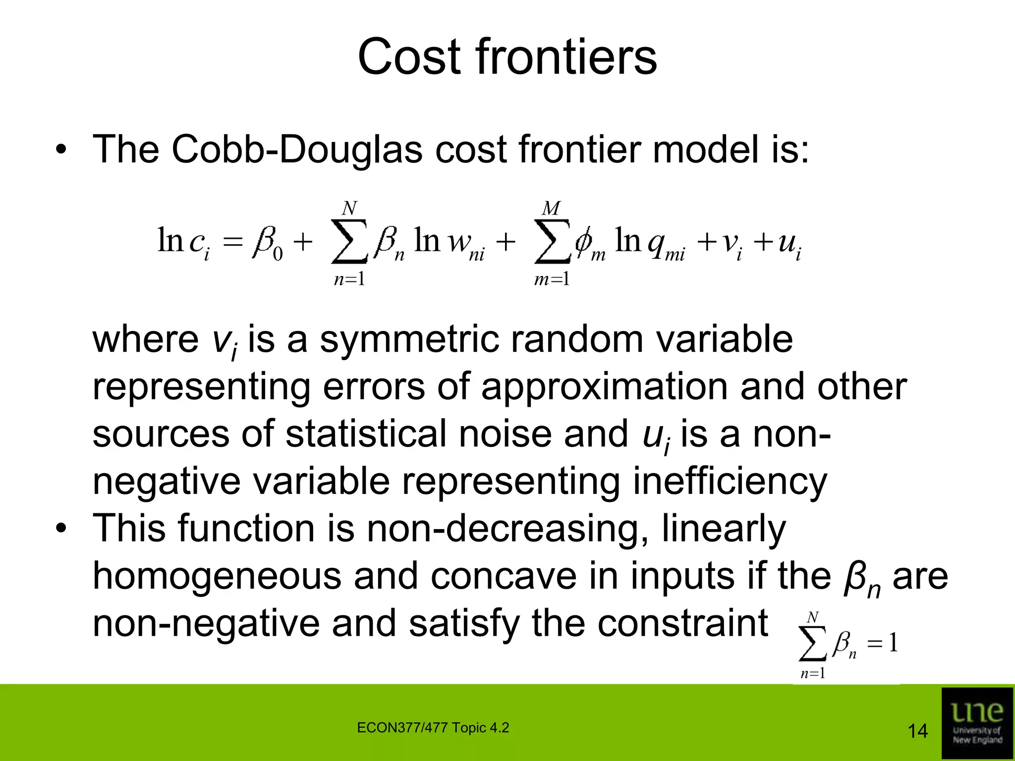
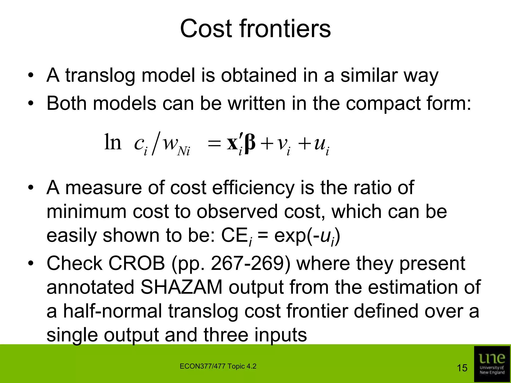
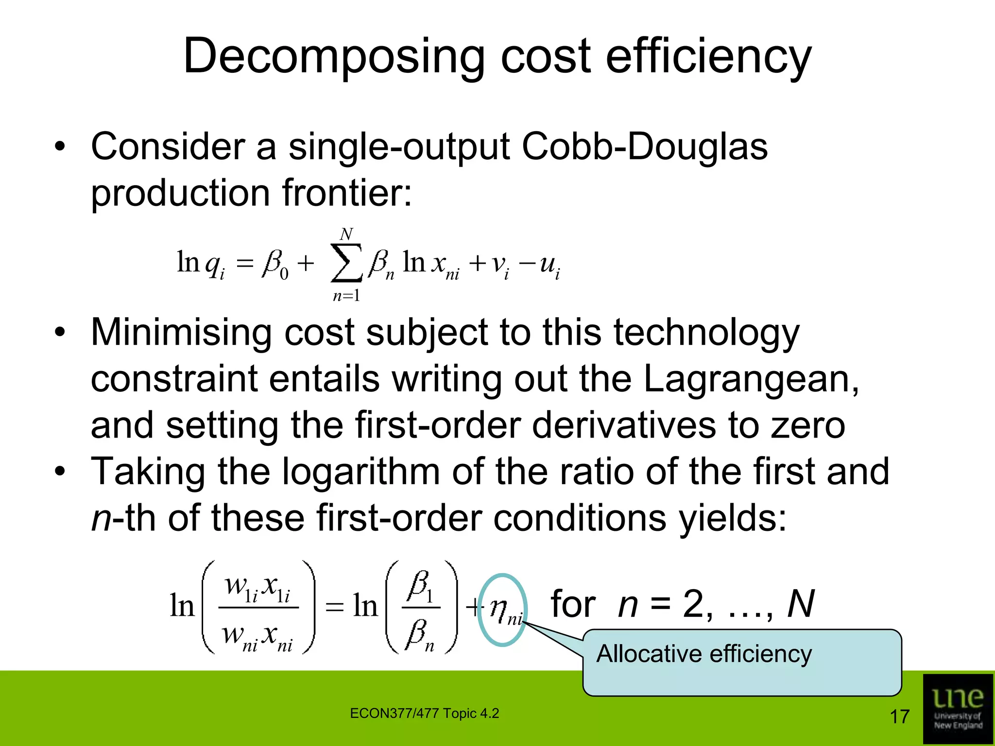
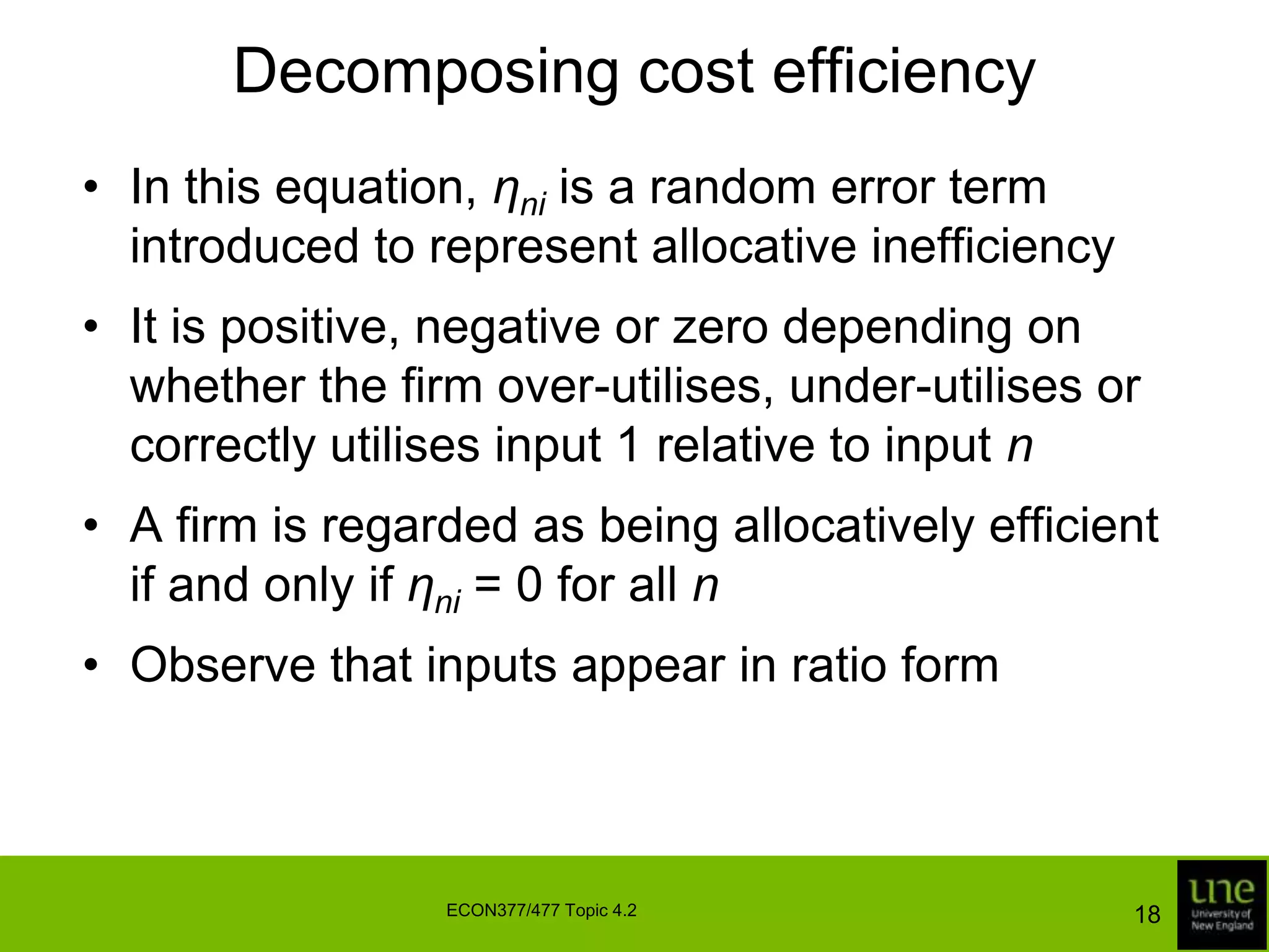
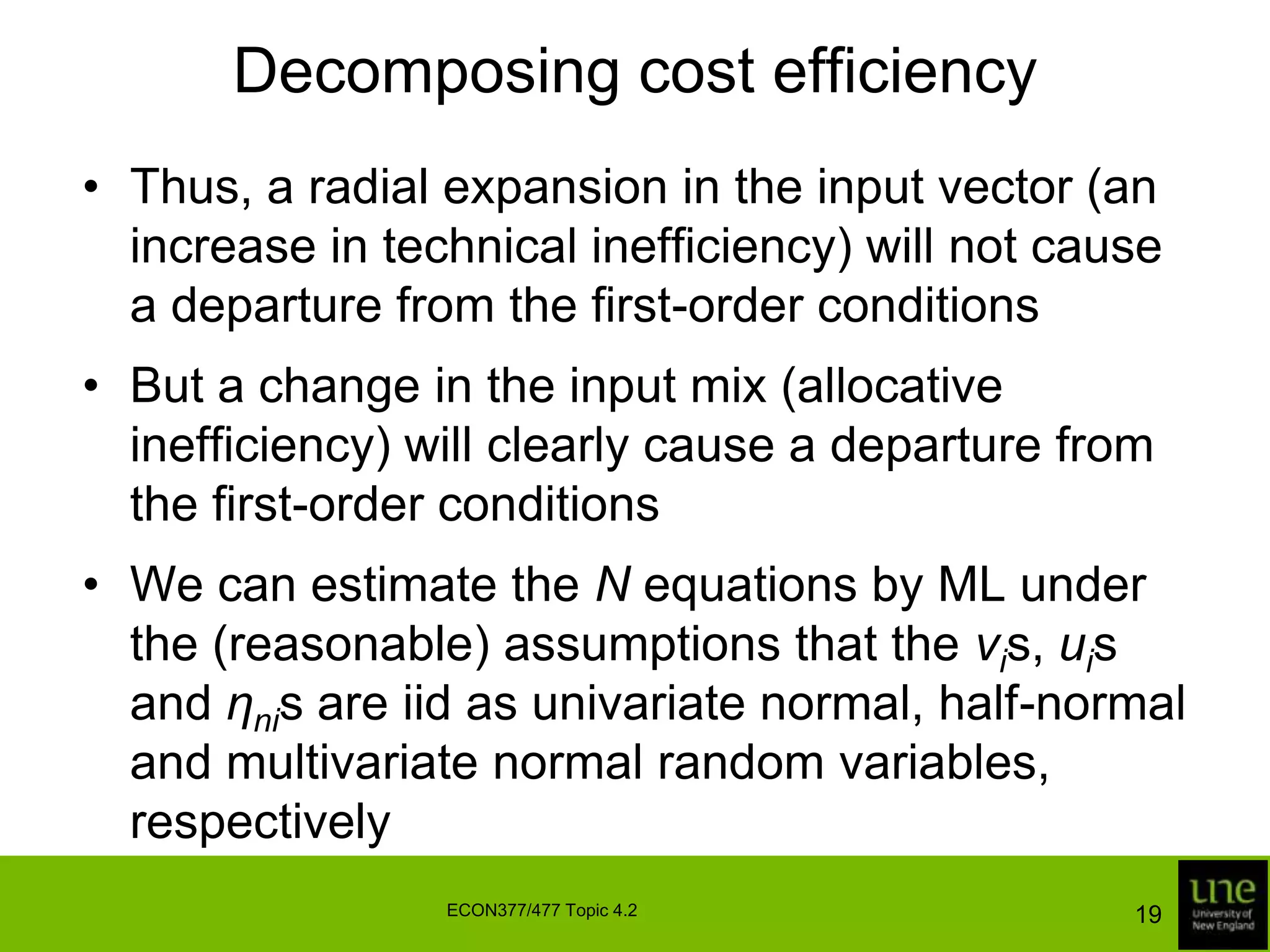
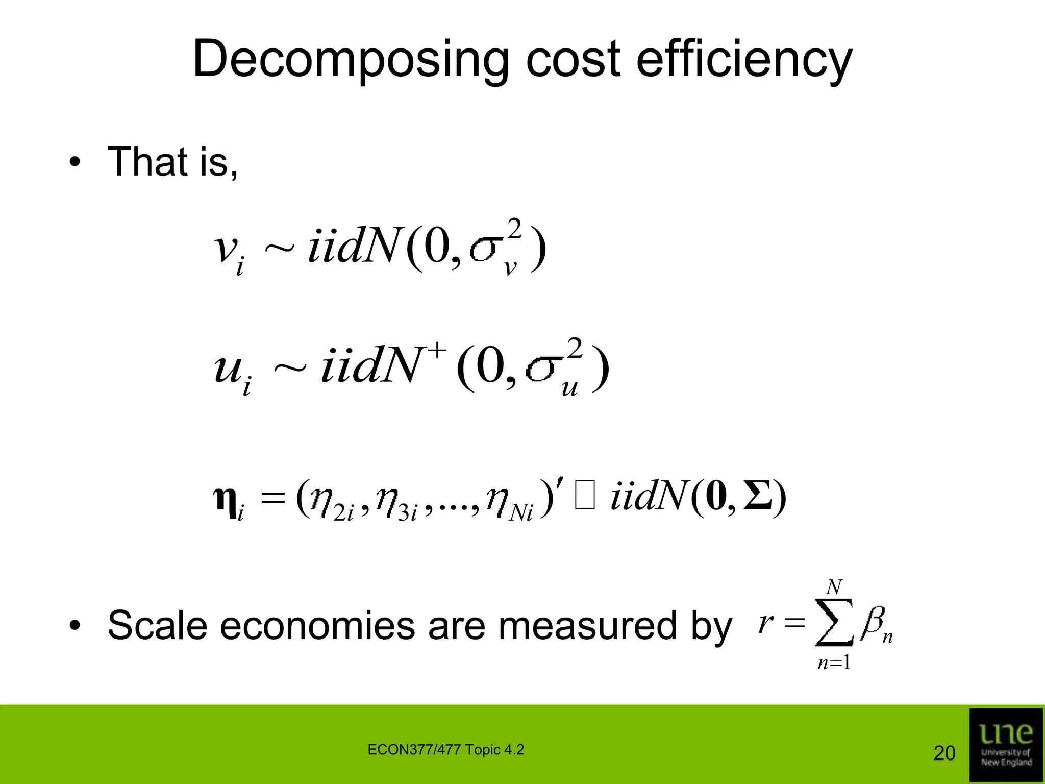
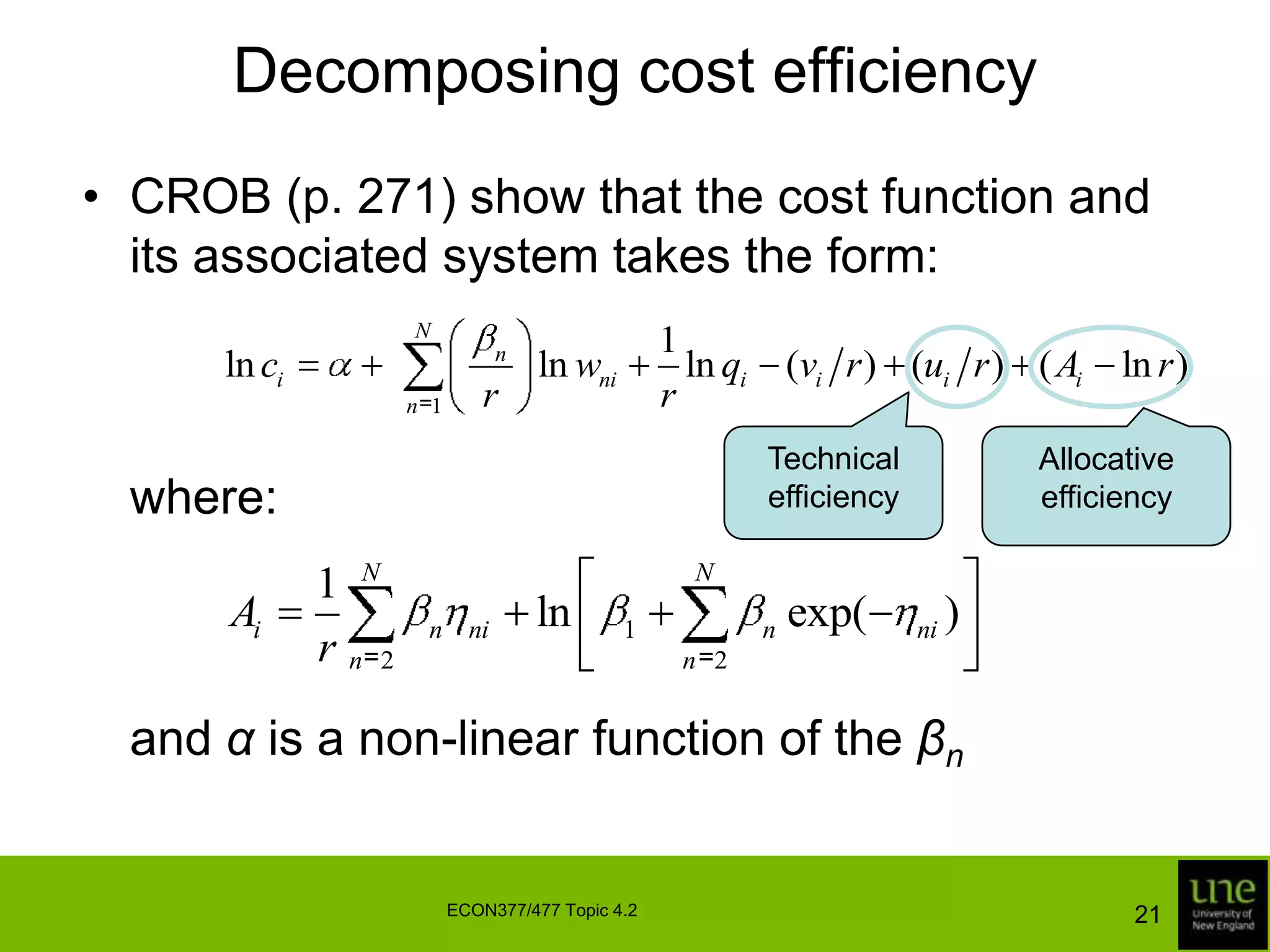
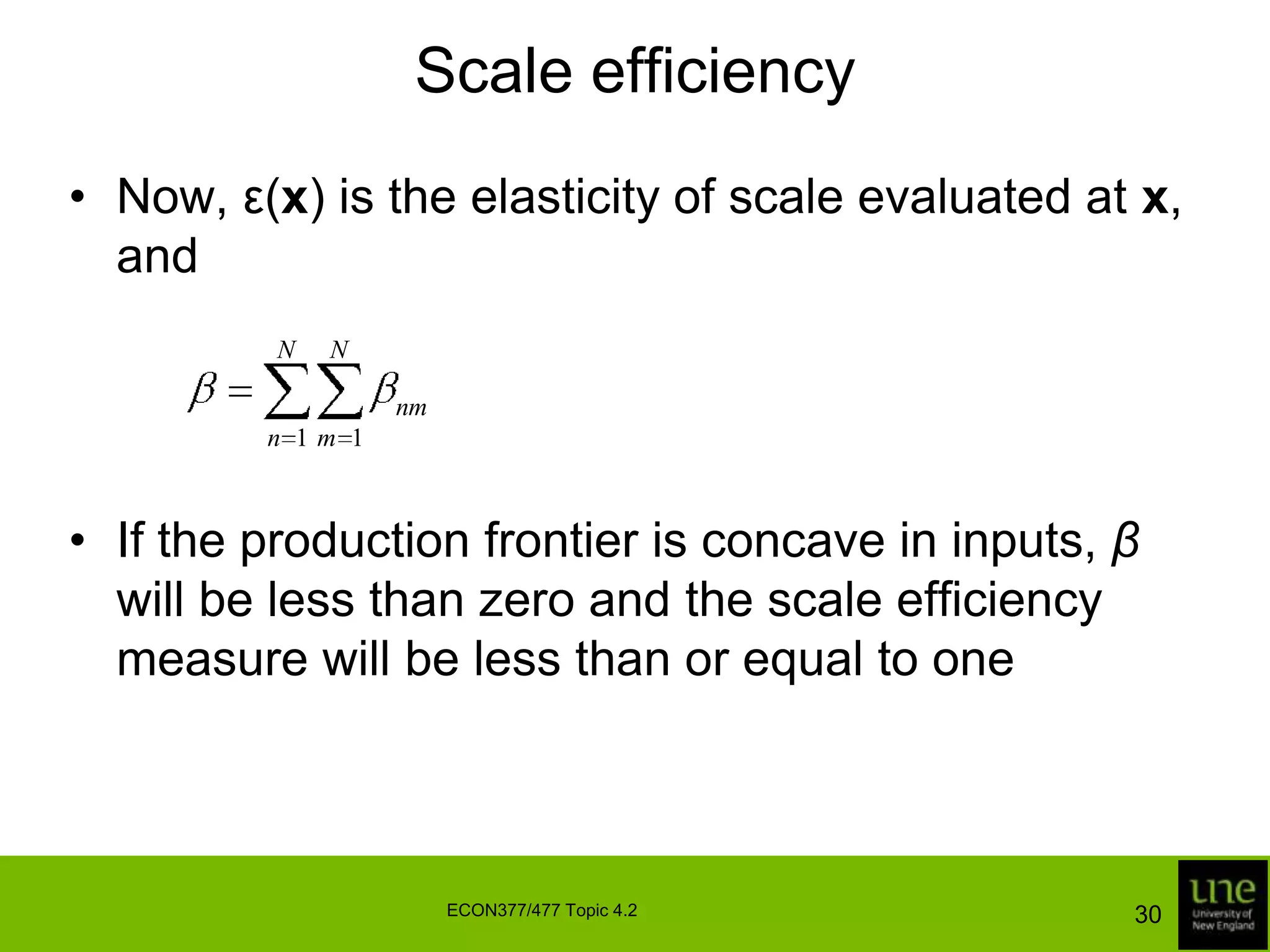
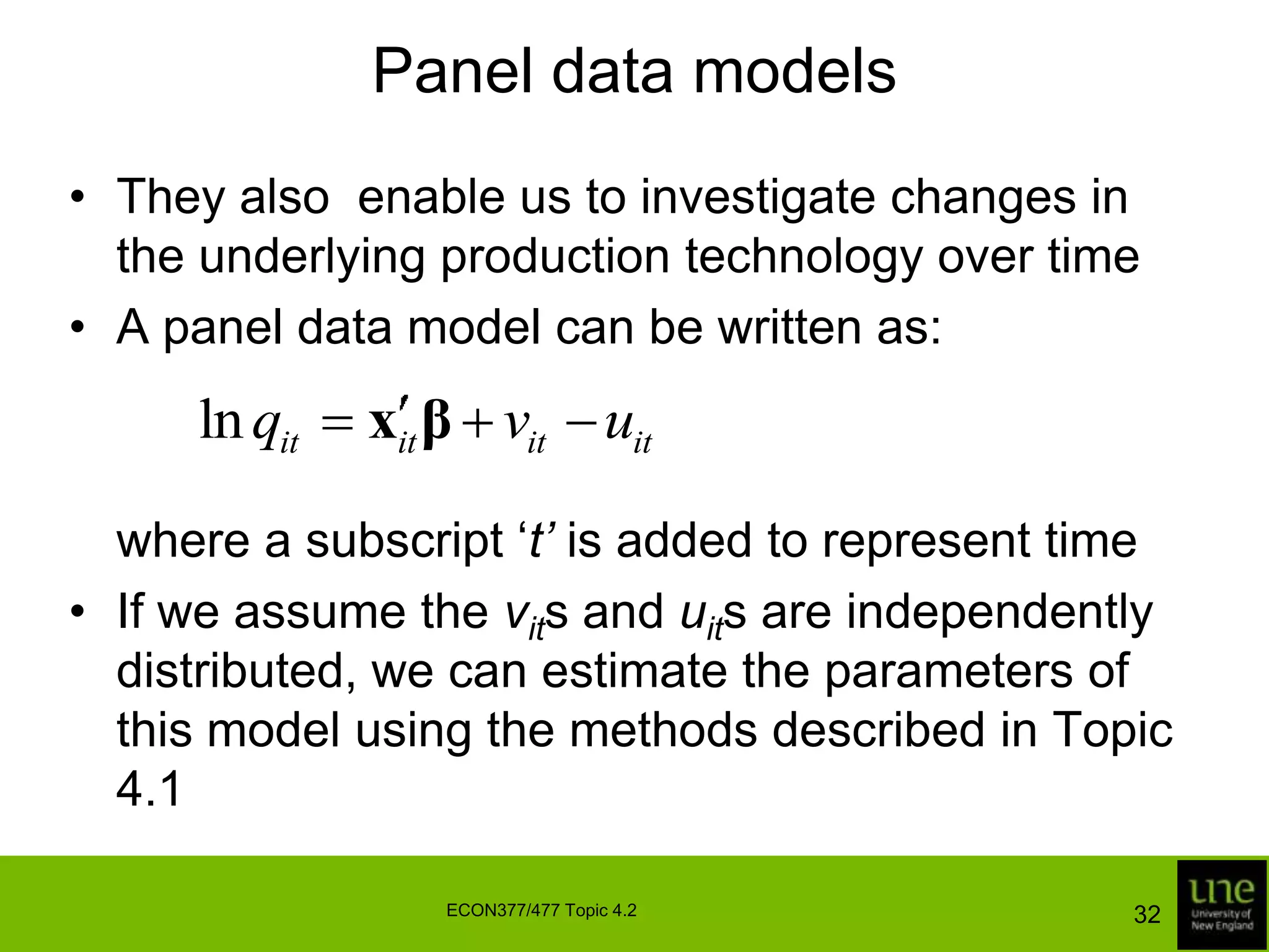
ECON 377/477
Topic 4.2Stochastic Frontier AnalysisPart 2
OutlineDistance functionsCost frontiersDecomposing cost efficiencyScale efficiencyPanel data modelsAccounting for the production environmentConclusions3ECON377/477 Topic 4.2
Distance functionsDistance functions can be used to estimate the characteristics of multiple-output production technologies in cases where we have no price information and/or it is inappropriate to assume firms minimise costs or maximise revenuesExamples arise when an industry is regulatedInput distance functions tend to be used instead of output distance functions when firms have more control over inputs than outputs, and vice versaWe consider only input distance functions4ECON377/477 Topic 4.2
Distance functionsAssume we have access to cross-sectional data on I firmsAn input distance function defined over M outputs and N inputs takes the form	where xniis the n-th input of firm i; qmi is the m-th output; and diI ≥ 1 is the maximum amount by which the input vector can be radially contracted without changing the output vectorECON377/477 Topic 4.25
Distance functionsThe function dI(.) is non-decreasing, linearly homogeneous and concave in inputs, and non-increasing and quasi-concave in outputsThe first step in econometric estimation of an input distance function is to choose a functional form for dI(.)It is convenient to choose a functional form that expresses the log-distance as a linear function of (transformations of) inputs and outputs6ECON377/477 Topic 4.2
Distance functionsFor example, if we choose the Cobb-Douglas functional form then the model becomes	where viis a random variable introduced to account for errors of approximation and other sources of statistical noiseThis function is non-decreasing, linearly homogeneous and concave in inputs if βn ≥ 0 for all n and if7ECON377/477 Topic 4.2
Distance functionsIt is also quasi-concave in outputs if non-linear functions of the first- and second-order derivatives of diI with respect to the outputs are non-negativeEconometric estimation would be reasonably straightforward were it not for the fact that the dependent variable is unobserved8ECON377/477 Topic 4.2
Distance functionsSome substitution and re-arrangement enables us to obtain a homogeneity-constrained model	where                is a non-negative variable associated with technical inefficiencyOur decision to express ln diI as a linear function of inputs and outputs results in a model that is in the form of the stochastic production frontier9ECON377/477 Topic 4.2
Distance functionsThis model is discussed in Part 1 of this topicIt follows that we can estimate the parameters of the model using the ML technique that is also discussed in Part 1A radial input-oriented measure of technical efficiency is:But there are two common problems in the estimation of distance functions10ECON377/477 Topic 4.2
Distance functionsThese problems are:The explanatory variables may be correlated with the composite error termEstimated input distance functions often fail to satisfy the concavity and quasi-concavity properties implied by economic theoryA solution to the first problem is to estimate the model in an instrumental variables frameworkA solution to the second problem is to impose regularity conditions by estimating the model in a Bayesian framework11ECON377/477 Topic 4.2
Cost frontiersWhen price data are available and it is reasonable to assume firms minimise costs, we can estimate the economic characteristics of the production technology (and predict cost efficiency) using a cost frontierIn the case where we have cross-sectional data, the cost frontier model can be written in the general form		ci ≥ c(w1i, w2i, …, wNi, q1i, q2i, …, qMi)12ECON377/477 Topic 4.2
Cost frontiersIn this equation, ci is the observed cost of firm i,wni is the n-th input price and qmi is the m-th outputNote that c(.) is a cost function that is non-decreasing, linearly homogeneous and concave in pricesThe implication of the equation is that the observed cost is greater than or equal to the minimum costThe first step in estimating the relationship is to specify a functional form for c(.)13ECON377/477 Topic 4.2
Cost frontiersThe Cobb-Douglas cost frontier model is:	where viis a symmetric random variable representing errors of approximation and other sources of statistical noise and uiis a non-negative variable representing inefficiencyThis function is non-decreasing, linearly homogeneous and concave in inputs if the βn are non-negative and satisfy the constraint14ECON377/477 Topic 4.2
Cost frontiersA translog model is obtained in a similar wayBoth models can be written in the compact form:A measure of cost efficiency is the ratio of minimum cost to observed cost, which can be easily shown to be: CEi = exp(-ui)Check CROB (pp. 267-269) where they present annotated SHAZAM output from the estimation of a half-normal translog cost frontier defined over a single output and three inputs15ECON377/477 Topic 4.2
Decomposing cost efficiencyWhen we have data on input quantities or cost-shares, cost efficiency can be decomposed into technical and allocative efficiency componentsOne approach involves estimating a cost frontier together with a subset of cost-share equationsWe focus on a slightly different decomposition method, estimating a production frontier together with a subset of the first-order conditions for cost minimisation16ECON377/477 Topic 4.2
Decomposing cost efficiencyConsider a single-output Cobb-Douglas production frontier:Minimising cost subject to this technology constraint entails writing out the Lagrangean, and setting the first-order derivatives to zeroTaking the logarithm of the ratio of the first and n-th of these first-order conditions yields:for  n = 2, …, NAllocative efficiency17ECON377/477 Topic 4.2
Decomposing cost efficiencyIn this equation, ηniis a random error term introduced to represent allocative inefficiencyIt is positive, negative or zero depending on whether the firm over-utilises, under-utilises or correctly utilises input 1 relative to input nA firm is regarded as being allocatively efficient if and only if ηni= 0 for all nObserve that inputs appear in ratio form18ECON377/477 Topic 4.2
Decomposing cost efficiencyThus, a radial expansion in the input vector (an increase in technical inefficiency) will not cause a departure from the first-order conditionsBut a change in the input mix (allocative inefficiency) will clearly cause a departure from the first-order conditionsWe can estimate the N equations by ML under the (reasonable) assumptions that the vis, uis and ηnis are iid as univariate normal, half-normal and multivariate normal random variables, respectively19ECON377/477 Topic 4.2
Decomposing cost efficiencyThat is,Scale economies are measured by20ECON377/477 Topic 4.2
Decomposing cost efficiencyCROB (p. 271) show that the cost function and its associated system takes the form:	where:	and α is a non-linear function of the βnTechnical efficiencyAllocative efficiency21ECON377/477 Topic 4.2
Decomposing cost efficiencyThe term ui/r measures the increase in the log-cost due to technical inefficiencyThe term Ai – ln r measures the increase due to allocative inefficiencyA measure of cost efficiency is the ratio of minimum cost to observed cost:CEi = CTEi × CAEi	where the component CTEi = exp(–ui/r) is due to technical inefficiency, and the component CAEi = exp(ln r – Ai) is due to allocative inefficiency22ECON377/477 Topic 4.2
Decomposing cost efficiencyWe can obtain point predictions for CTEi and CAEi by substituting predictions for ui and ηni into these expressionsIf the technology exhibits constant returns to scale (r = 1), then:		CTEi  = TEi = exp(–ui)		CAEi= AEi ≡ exp(–Ai)Thus, CEi = TEi × AEi, which is the familiar expression from Topic 223ECON377/477 Topic 4.2
Decomposing cost efficiencyCROB illustrate the method and present annotated SHAZAM output in Table 10.2 from the estimation of a three-input Cobb-Douglas production frontier and decomposition of cost efficiency into its two componentsFor simplicity, they estimate the production frontier in a single-equation framework, although more efficient estimators could be obtained by estimating the frontier in a seemingly unrelated regression framework24ECON377/477 Topic 4.2
Scale efficiencyTo measure scale efficiency, we must have a measure of productivity and a method for identifying the most productive scale size (MPSS)In the case of a single-input production function, we can measure productivity using the APThe MPSS is the point of maximum AP(x)The first-order condition for a maximum can be easily rearranged to show that the MPSS is the point where the elasticity of scale is 1 and the firm experiences local constant returns to scale25ECON377/477 Topic 4.2
Scale efficiencyTo measure scale efficiency, we set the elasticity of scale to 1 and solve for the MPSS, denoted x*Scale efficiency at any input level x is:This procedure generalises to the multiple-input case, although a measure of productivity is a little more difficult to conceptualise26ECON377/477 Topic 4.2
Scale efficiencyThink of the input vector x as one unit of a composite input, so that kx represents k units of inputA measure of productivity is the ray average product (RAP):Set the elasticity of scale to 1 and solve for the optimal number of units of the composite input, denoted k*27ECON377/477 Topic 4.2
Scale efficiencyA measure of scale efficiency at input level kx is:	or, if k = 1:A solution can be obtained for a translog functional form and the associated measure of scale efficiency derived28ECON377/477 Topic 4.2
Scale efficiencyIf the production frontier takes the translog form	 the scale efficiency measure becomes	where29ECON377/477 Topic 4.2
Scale efficiencyNow, ε(x) is the elasticity of scale evaluated at x, andIf the production frontier is concave in inputs, β will be less than zero and the scale efficiency measure will be less than or equal to one30ECON377/477 Topic 4.2
Panel data modelsWe now extend discussion of frontier models to the case where panel data are availablePanel data sets enable us to obtain more efficient estimators of the unknown parameters and more efficient predictors of technical efficienciesThey often allow us to:relax some of the strong distributional assumptions
obtain consistent predictions of TEs
investigate changes in technical efficiencies31ECON377/477 Topic 4.2
Panel data modelsThey also  enable us to investigate changes in the underlying production technology over timeA panel data model can be written as:	where a subscript ‘t’ is added to represent timeIf we assume the vits and uits are independently distributed, we can estimate the parameters of this model using the methods described in Topic 4.132ECON377/477 Topic 4.2
Panel data modelsA problem with assuming the uits are independently distributed is that we fail to reap any of the benefits listed aboveMoreover, for many industries the independence assumption is unrealistic – all other things being equal, we expect efficient firms to remain reasonably efficient from period to period, and we hope that inefficient firms improve their efficiency levels over timeFor these reasons, we need to impose some structure on the inefficiency effects33ECON377/477 Topic 4.2
Panel data modelsIt is common to classify different structures on the inefficiency effects according to whether they are time-invariant or time-varyingOne of the simplest structures we can impose on the inefficiency effects is		uit = uii = 1, …, I; t = 1, …., T	where ui is treated as either a fixed parameter or a random variableThese models are known as the fixed effects model and random effects model, respectively34ECON377/477 Topic 4.2
Panel data modelsThe fixed effects model can be estimated in a standard regression framework using dummy variablesThe estimated model can only be used to measure efficiency relative to the most efficient firm in the sample so our estimates may be unreliable if the number of firms is smallThe random effects model can be estimated using either least squares or ML techniques35ECON377/477 Topic 4.2
Panel data modelsThe ML approach involves making stronger distributional assumptions concerning the uisEstimating models in a random effects framework using the ML method allows us to disentangle the effects of inefficiency and technological change36ECON377/477 Topic 4.2
Panel data modelsThe likelihood function for this model is a generalisation of the likelihood function for the half-normal stochastic frontier model discussed in Topic 4.1Formulas for firm-specific and industry efficiencies are also generalisations of the formulas presented in Topic 4.1The hypothesis testing procedures discussed in Topic 4.1 are also applicable37ECON377/477 Topic 4.2
Panel data modelsModels with time-invariant inefficiency effects can be conveniently estimated using FRONTIER and LIMDEPCROB illustrate this estimation in Table 10.3, which contains annotated FRONTIER output from the estimation of a truncated-normal frontierNote that significant differences exist between the first-order coefficient estimates reported in this table and those reported in Table 9.6 where no account is taken of the panel nature of the data38ECON377/477 Topic 4.2
Panel data modelsTwo models that allow for time-varying technical inefficiency take the form:	where α, β and η are unknown parameters to be estimatedThe Battese and Coelli function involves only one unknown parameter, and is less flexibleKumbhakar modelBattese and Coelli model39ECON377/477 Topic 4.2
Panel data modelsA limitation of both functions is that they do not allow for a change in the rank ordering of firms over timeThe firm that is ranked n-th at the first time period is always ranked n-thThat is, if ui < uj, then  	for all t40ECON377/477 Topic 4.2
Panel data modelsThe Kumbhakar and Battese and Coelli models can both be estimated under the assumption that ui has a truncated normal distribution:Again, the likelihood function is a generalisation of the likelihood function for the half-normal stochastic frontier model, as are formulas for firm-specific and industry efficienciesHypotheses concerning individual coefficients can be tested using a z test or LR test, but they are usually tested using an LR test if there is more than one coefficient in the test41ECON377/477 Topic 4.2
Panel data modelsNull hypotheses of special interest areH0: α = β = 0 or H0: η = 0 (time-invariant efficiency effects)
H0: µ = 0 (half-normal inefficiency effects at time period T)CROB present annotated FRONTIER output from the estimation of a frontier in Table 10.4They are unable to reject both null hypotheses that the technological change effect is zero and η = 042ECON377/477 Topic 4.2
Panel data modelsThese hypothesis test results suggest that the model is having difficulty distinguishing between output increases due to technological progress and output increases due to improvements in technical efficiencySeveral more flexible models are discussed in the efficiency literatureNotably, Cuesta (2000) specifies a model of the form  that generalises the Battese and Coelli model and allows the temporal pattern of inefficiency effects to vary across firms 43ECON377/477 Topic 4.2
Accounting for the production environmentThe ability of a manager to convert inputs into outputs is often influenced by exogenous variables that characterise the environment in which production takes placeIt is useful to distinguish between non-stochastic variables that are observable at the time key production decisions are made and unforeseen stochastic variables that can be regarded as sources of production risk (events of any type that might lead managers to seek some form of liability insurance)44ECON377/477 Topic 4.2
Accounting for the production environmentThe simplest way to account for non-stochastic environmental variables is to incorporate them directly into the non-stochastic component of the production frontierIn the case of cross-sectional data this leads to a model of the form:	where zi is a vector of (transformations of) environmental variables and γ is a vector of unknown parameters45ECON377/477 Topic 4.2
Accounting for the production environmentThis model has exactly the same error structure as the conventional stochastic frontier model discussed in Topic 4.1Thus, all the estimators and testing procedures discussed in that part of the topic are availableOur predictions of firm-specific technical efficiency now vary with both the traditional inputs and the environmental variables46ECON377/477 Topic 4.2
Accounting for the production environmentThe preferred method to deal with observable environmental variables is to allow them directly to influence the stochastic component of the production frontierAssumeand47ECON377/477 Topic 4.2
Accounting for the production environmentThe inefficiency effects in the frontier model have distributions that vary with zi, so they are no longer identically distributedThe likelihood function is a generalisation of the likelihood function for the conventional model, as are measures of firm-specific and industry efficiencyThe model has also been generalised to the panel data case48ECON377/477 Topic 4.2
Accounting for the production environmentA simple way to account for production risk is to append another random variable to the frontier model to represent the combined effects of any variables that are unobserved at the time input decisions are madeIf we assume this random variable has a symmetric distribution, then it is difficult to distinguish it from the noise viAlternatively, if we assume it has a non-negative distribution, it is difficult to distinguish it from the inefficiency effect ui49ECON377/477 Topic 4.2
Accounting for the production environmentThis suggests that, for all intents and purposes, we can persist with the conventional stochastic frontier model, although we should recognise that the two error components now measure the effects of noise, inefficiency and riskBut the conventional frontier model has two undesirable risk propertiesThe signs of the MPs are the same as the signs of the associated marginal risks
The model does not permit substitutability between state-contingent outputs50ECON377/477 Topic 4.2
Accounting for the production environmentOne way to overcome the first problem is to assume the composed error term is heteroskedasticOne way to allow for substitution between state-contingent outputs is to estimate a state-contingent stochastic frontier of the form	where βj is a vector of unknown parameters and viand ui represent noise and inefficiency, respectively (but not risk)51ECON377/477 Topic 4.2

Topic 4.2

  • 1.
  • 2.
  • 3.
    OutlineDistance functionsCost frontiersDecomposingcost efficiencyScale efficiencyPanel data modelsAccounting for the production environmentConclusions3ECON377/477 Topic 4.2
  • 4.
    Distance functionsDistance functionscan be used to estimate the characteristics of multiple-output production technologies in cases where we have no price information and/or it is inappropriate to assume firms minimise costs or maximise revenuesExamples arise when an industry is regulatedInput distance functions tend to be used instead of output distance functions when firms have more control over inputs than outputs, and vice versaWe consider only input distance functions4ECON377/477 Topic 4.2
  • 5.
    Distance functionsAssume wehave access to cross-sectional data on I firmsAn input distance function defined over M outputs and N inputs takes the form where xniis the n-th input of firm i; qmi is the m-th output; and diI ≥ 1 is the maximum amount by which the input vector can be radially contracted without changing the output vectorECON377/477 Topic 4.25
  • 6.
    Distance functionsThe functiondI(.) is non-decreasing, linearly homogeneous and concave in inputs, and non-increasing and quasi-concave in outputsThe first step in econometric estimation of an input distance function is to choose a functional form for dI(.)It is convenient to choose a functional form that expresses the log-distance as a linear function of (transformations of) inputs and outputs6ECON377/477 Topic 4.2
  • 7.
    Distance functionsFor example,if we choose the Cobb-Douglas functional form then the model becomes where viis a random variable introduced to account for errors of approximation and other sources of statistical noiseThis function is non-decreasing, linearly homogeneous and concave in inputs if βn ≥ 0 for all n and if7ECON377/477 Topic 4.2
  • 8.
    Distance functionsIt isalso quasi-concave in outputs if non-linear functions of the first- and second-order derivatives of diI with respect to the outputs are non-negativeEconometric estimation would be reasonably straightforward were it not for the fact that the dependent variable is unobserved8ECON377/477 Topic 4.2
  • 9.
    Distance functionsSome substitutionand re-arrangement enables us to obtain a homogeneity-constrained model where is a non-negative variable associated with technical inefficiencyOur decision to express ln diI as a linear function of inputs and outputs results in a model that is in the form of the stochastic production frontier9ECON377/477 Topic 4.2
  • 10.
    Distance functionsThis modelis discussed in Part 1 of this topicIt follows that we can estimate the parameters of the model using the ML technique that is also discussed in Part 1A radial input-oriented measure of technical efficiency is:But there are two common problems in the estimation of distance functions10ECON377/477 Topic 4.2
  • 11.
    Distance functionsThese problemsare:The explanatory variables may be correlated with the composite error termEstimated input distance functions often fail to satisfy the concavity and quasi-concavity properties implied by economic theoryA solution to the first problem is to estimate the model in an instrumental variables frameworkA solution to the second problem is to impose regularity conditions by estimating the model in a Bayesian framework11ECON377/477 Topic 4.2
  • 12.
    Cost frontiersWhen pricedata are available and it is reasonable to assume firms minimise costs, we can estimate the economic characteristics of the production technology (and predict cost efficiency) using a cost frontierIn the case where we have cross-sectional data, the cost frontier model can be written in the general form ci ≥ c(w1i, w2i, …, wNi, q1i, q2i, …, qMi)12ECON377/477 Topic 4.2
  • 13.
    Cost frontiersIn thisequation, ci is the observed cost of firm i,wni is the n-th input price and qmi is the m-th outputNote that c(.) is a cost function that is non-decreasing, linearly homogeneous and concave in pricesThe implication of the equation is that the observed cost is greater than or equal to the minimum costThe first step in estimating the relationship is to specify a functional form for c(.)13ECON377/477 Topic 4.2
  • 14.
    Cost frontiersThe Cobb-Douglascost frontier model is: where viis a symmetric random variable representing errors of approximation and other sources of statistical noise and uiis a non-negative variable representing inefficiencyThis function is non-decreasing, linearly homogeneous and concave in inputs if the βn are non-negative and satisfy the constraint14ECON377/477 Topic 4.2
  • 15.
    Cost frontiersA translogmodel is obtained in a similar wayBoth models can be written in the compact form:A measure of cost efficiency is the ratio of minimum cost to observed cost, which can be easily shown to be: CEi = exp(-ui)Check CROB (pp. 267-269) where they present annotated SHAZAM output from the estimation of a half-normal translog cost frontier defined over a single output and three inputs15ECON377/477 Topic 4.2
  • 16.
    Decomposing cost efficiencyWhenwe have data on input quantities or cost-shares, cost efficiency can be decomposed into technical and allocative efficiency componentsOne approach involves estimating a cost frontier together with a subset of cost-share equationsWe focus on a slightly different decomposition method, estimating a production frontier together with a subset of the first-order conditions for cost minimisation16ECON377/477 Topic 4.2
  • 17.
    Decomposing cost efficiencyConsidera single-output Cobb-Douglas production frontier:Minimising cost subject to this technology constraint entails writing out the Lagrangean, and setting the first-order derivatives to zeroTaking the logarithm of the ratio of the first and n-th of these first-order conditions yields:for n = 2, …, NAllocative efficiency17ECON377/477 Topic 4.2
  • 18.
    Decomposing cost efficiencyInthis equation, ηniis a random error term introduced to represent allocative inefficiencyIt is positive, negative or zero depending on whether the firm over-utilises, under-utilises or correctly utilises input 1 relative to input nA firm is regarded as being allocatively efficient if and only if ηni= 0 for all nObserve that inputs appear in ratio form18ECON377/477 Topic 4.2
  • 19.
    Decomposing cost efficiencyThus,a radial expansion in the input vector (an increase in technical inefficiency) will not cause a departure from the first-order conditionsBut a change in the input mix (allocative inefficiency) will clearly cause a departure from the first-order conditionsWe can estimate the N equations by ML under the (reasonable) assumptions that the vis, uis and ηnis are iid as univariate normal, half-normal and multivariate normal random variables, respectively19ECON377/477 Topic 4.2
  • 20.
    Decomposing cost efficiencyThatis,Scale economies are measured by20ECON377/477 Topic 4.2
  • 21.
    Decomposing cost efficiencyCROB(p. 271) show that the cost function and its associated system takes the form: where: and α is a non-linear function of the βnTechnical efficiencyAllocative efficiency21ECON377/477 Topic 4.2
  • 22.
    Decomposing cost efficiencyTheterm ui/r measures the increase in the log-cost due to technical inefficiencyThe term Ai – ln r measures the increase due to allocative inefficiencyA measure of cost efficiency is the ratio of minimum cost to observed cost:CEi = CTEi × CAEi where the component CTEi = exp(–ui/r) is due to technical inefficiency, and the component CAEi = exp(ln r – Ai) is due to allocative inefficiency22ECON377/477 Topic 4.2
  • 23.
    Decomposing cost efficiencyWecan obtain point predictions for CTEi and CAEi by substituting predictions for ui and ηni into these expressionsIf the technology exhibits constant returns to scale (r = 1), then: CTEi = TEi = exp(–ui) CAEi= AEi ≡ exp(–Ai)Thus, CEi = TEi × AEi, which is the familiar expression from Topic 223ECON377/477 Topic 4.2
  • 24.
    Decomposing cost efficiencyCROBillustrate the method and present annotated SHAZAM output in Table 10.2 from the estimation of a three-input Cobb-Douglas production frontier and decomposition of cost efficiency into its two componentsFor simplicity, they estimate the production frontier in a single-equation framework, although more efficient estimators could be obtained by estimating the frontier in a seemingly unrelated regression framework24ECON377/477 Topic 4.2
  • 25.
    Scale efficiencyTo measurescale efficiency, we must have a measure of productivity and a method for identifying the most productive scale size (MPSS)In the case of a single-input production function, we can measure productivity using the APThe MPSS is the point of maximum AP(x)The first-order condition for a maximum can be easily rearranged to show that the MPSS is the point where the elasticity of scale is 1 and the firm experiences local constant returns to scale25ECON377/477 Topic 4.2
  • 26.
    Scale efficiencyTo measurescale efficiency, we set the elasticity of scale to 1 and solve for the MPSS, denoted x*Scale efficiency at any input level x is:This procedure generalises to the multiple-input case, although a measure of productivity is a little more difficult to conceptualise26ECON377/477 Topic 4.2
  • 27.
    Scale efficiencyThink ofthe input vector x as one unit of a composite input, so that kx represents k units of inputA measure of productivity is the ray average product (RAP):Set the elasticity of scale to 1 and solve for the optimal number of units of the composite input, denoted k*27ECON377/477 Topic 4.2
  • 28.
    Scale efficiencyA measureof scale efficiency at input level kx is: or, if k = 1:A solution can be obtained for a translog functional form and the associated measure of scale efficiency derived28ECON377/477 Topic 4.2
  • 29.
    Scale efficiencyIf theproduction frontier takes the translog form the scale efficiency measure becomes where29ECON377/477 Topic 4.2
  • 30.
    Scale efficiencyNow, ε(x)is the elasticity of scale evaluated at x, andIf the production frontier is concave in inputs, β will be less than zero and the scale efficiency measure will be less than or equal to one30ECON377/477 Topic 4.2
  • 31.
    Panel data modelsWenow extend discussion of frontier models to the case where panel data are availablePanel data sets enable us to obtain more efficient estimators of the unknown parameters and more efficient predictors of technical efficienciesThey often allow us to:relax some of the strong distributional assumptions
  • 32.
  • 33.
    investigate changes intechnical efficiencies31ECON377/477 Topic 4.2
  • 34.
    Panel data modelsTheyalso enable us to investigate changes in the underlying production technology over timeA panel data model can be written as: where a subscript ‘t’ is added to represent timeIf we assume the vits and uits are independently distributed, we can estimate the parameters of this model using the methods described in Topic 4.132ECON377/477 Topic 4.2
  • 35.
    Panel data modelsAproblem with assuming the uits are independently distributed is that we fail to reap any of the benefits listed aboveMoreover, for many industries the independence assumption is unrealistic – all other things being equal, we expect efficient firms to remain reasonably efficient from period to period, and we hope that inefficient firms improve their efficiency levels over timeFor these reasons, we need to impose some structure on the inefficiency effects33ECON377/477 Topic 4.2
  • 36.
    Panel data modelsItis common to classify different structures on the inefficiency effects according to whether they are time-invariant or time-varyingOne of the simplest structures we can impose on the inefficiency effects is uit = uii = 1, …, I; t = 1, …., T where ui is treated as either a fixed parameter or a random variableThese models are known as the fixed effects model and random effects model, respectively34ECON377/477 Topic 4.2
  • 37.
    Panel data modelsThefixed effects model can be estimated in a standard regression framework using dummy variablesThe estimated model can only be used to measure efficiency relative to the most efficient firm in the sample so our estimates may be unreliable if the number of firms is smallThe random effects model can be estimated using either least squares or ML techniques35ECON377/477 Topic 4.2
  • 38.
    Panel data modelsTheML approach involves making stronger distributional assumptions concerning the uisEstimating models in a random effects framework using the ML method allows us to disentangle the effects of inefficiency and technological change36ECON377/477 Topic 4.2
  • 39.
    Panel data modelsThelikelihood function for this model is a generalisation of the likelihood function for the half-normal stochastic frontier model discussed in Topic 4.1Formulas for firm-specific and industry efficiencies are also generalisations of the formulas presented in Topic 4.1The hypothesis testing procedures discussed in Topic 4.1 are also applicable37ECON377/477 Topic 4.2
  • 40.
    Panel data modelsModelswith time-invariant inefficiency effects can be conveniently estimated using FRONTIER and LIMDEPCROB illustrate this estimation in Table 10.3, which contains annotated FRONTIER output from the estimation of a truncated-normal frontierNote that significant differences exist between the first-order coefficient estimates reported in this table and those reported in Table 9.6 where no account is taken of the panel nature of the data38ECON377/477 Topic 4.2
  • 41.
    Panel data modelsTwomodels that allow for time-varying technical inefficiency take the form: where α, β and η are unknown parameters to be estimatedThe Battese and Coelli function involves only one unknown parameter, and is less flexibleKumbhakar modelBattese and Coelli model39ECON377/477 Topic 4.2
  • 42.
    Panel data modelsAlimitation of both functions is that they do not allow for a change in the rank ordering of firms over timeThe firm that is ranked n-th at the first time period is always ranked n-thThat is, if ui < uj, then for all t40ECON377/477 Topic 4.2
  • 43.
    Panel data modelsTheKumbhakar and Battese and Coelli models can both be estimated under the assumption that ui has a truncated normal distribution:Again, the likelihood function is a generalisation of the likelihood function for the half-normal stochastic frontier model, as are formulas for firm-specific and industry efficienciesHypotheses concerning individual coefficients can be tested using a z test or LR test, but they are usually tested using an LR test if there is more than one coefficient in the test41ECON377/477 Topic 4.2
  • 44.
    Panel data modelsNullhypotheses of special interest areH0: α = β = 0 or H0: η = 0 (time-invariant efficiency effects)
  • 45.
    H0: µ =0 (half-normal inefficiency effects at time period T)CROB present annotated FRONTIER output from the estimation of a frontier in Table 10.4They are unable to reject both null hypotheses that the technological change effect is zero and η = 042ECON377/477 Topic 4.2
  • 46.
    Panel data modelsThesehypothesis test results suggest that the model is having difficulty distinguishing between output increases due to technological progress and output increases due to improvements in technical efficiencySeveral more flexible models are discussed in the efficiency literatureNotably, Cuesta (2000) specifies a model of the form that generalises the Battese and Coelli model and allows the temporal pattern of inefficiency effects to vary across firms 43ECON377/477 Topic 4.2
  • 47.
    Accounting for theproduction environmentThe ability of a manager to convert inputs into outputs is often influenced by exogenous variables that characterise the environment in which production takes placeIt is useful to distinguish between non-stochastic variables that are observable at the time key production decisions are made and unforeseen stochastic variables that can be regarded as sources of production risk (events of any type that might lead managers to seek some form of liability insurance)44ECON377/477 Topic 4.2
  • 48.
    Accounting for theproduction environmentThe simplest way to account for non-stochastic environmental variables is to incorporate them directly into the non-stochastic component of the production frontierIn the case of cross-sectional data this leads to a model of the form: where zi is a vector of (transformations of) environmental variables and γ is a vector of unknown parameters45ECON377/477 Topic 4.2
  • 49.
    Accounting for theproduction environmentThis model has exactly the same error structure as the conventional stochastic frontier model discussed in Topic 4.1Thus, all the estimators and testing procedures discussed in that part of the topic are availableOur predictions of firm-specific technical efficiency now vary with both the traditional inputs and the environmental variables46ECON377/477 Topic 4.2
  • 50.
    Accounting for theproduction environmentThe preferred method to deal with observable environmental variables is to allow them directly to influence the stochastic component of the production frontierAssumeand47ECON377/477 Topic 4.2
  • 51.
    Accounting for theproduction environmentThe inefficiency effects in the frontier model have distributions that vary with zi, so they are no longer identically distributedThe likelihood function is a generalisation of the likelihood function for the conventional model, as are measures of firm-specific and industry efficiencyThe model has also been generalised to the panel data case48ECON377/477 Topic 4.2
  • 52.
    Accounting for theproduction environmentA simple way to account for production risk is to append another random variable to the frontier model to represent the combined effects of any variables that are unobserved at the time input decisions are madeIf we assume this random variable has a symmetric distribution, then it is difficult to distinguish it from the noise viAlternatively, if we assume it has a non-negative distribution, it is difficult to distinguish it from the inefficiency effect ui49ECON377/477 Topic 4.2
  • 53.
    Accounting for theproduction environmentThis suggests that, for all intents and purposes, we can persist with the conventional stochastic frontier model, although we should recognise that the two error components now measure the effects of noise, inefficiency and riskBut the conventional frontier model has two undesirable risk propertiesThe signs of the MPs are the same as the signs of the associated marginal risks
  • 54.
    The model doesnot permit substitutability between state-contingent outputs50ECON377/477 Topic 4.2
  • 55.
    Accounting for theproduction environmentOne way to overcome the first problem is to assume the composed error term is heteroskedasticOne way to allow for substitution between state-contingent outputs is to estimate a state-contingent stochastic frontier of the form where βj is a vector of unknown parameters and viand ui represent noise and inefficiency, respectively (but not risk)51ECON377/477 Topic 4.2
  • 56.
    Accounting for theproduction environmentThis model is identical to the conventional stochastic frontier model, except the coefficient vector βj is permitted to vary across risky states of nature, j = 1, …, JEstimation is complicated by the fact that states of nature are typically unobserved or data are sparseThis problem can be overcome by estimating the model in a Bayesian mixtures framework, and using this model to identify output shortfalls due to inefficiency and output shortfalls due to adverse conditions52ECON377/477 Topic 4.2
  • 57.
    ConclusionsTwo other possiblemethods for estimating multiple-output technologies are not discussedFirst, we can use profit frontiers when input and output prices are available and it is reasonable to assume firms maximise profitsMethods to estimate profit frontiers are similar to those available for estimating cost frontiersSecond, we can aggregate multiple outputs into a single output measure using index number methods, and estimate the technology in a conventional single-output framework53ECON377/477 Topic 4.2
  • 58.
    ConclusionsThe decision toestimate a distance function, cost frontier, profit frontier or single-output production frontier is one of the many decisions facing researchers who want to estimate efficiency using a parametric approachResearchers must also make choices concerning functional forms, error distributions, estimation methods and softwareThe need to make so many choices is often seen as a disadvantage of the parametric approach54ECON377/477 Topic 4.2
  • 59.
    ConclusionsWe have twosimple pieces of advice:Always make decisions on a case-by-case basisWhenever it is possible, explore alternative models and estimation methods and (formally or informally) assess the adequacy and robustness of the results obtained55ECON377/477 Topic 4.2