time synchronization and localization .pptx

1
MODULE IV
MODULE IV : TIME SYNCHRONIZATION
Time Synchronization: Clocks and the Synchronization Problem, Time
Synchronization in Wireless Sensor Networks, Basics of Time Synchronization,
Time Synchronization Protocols Localization: Ranging Techniques,
Range Based Localization, Range-Free Localization, Event Driven
Localization.

2
Time Synchronization
 In distributed systems, each node has its own clock and its own notion of
time.
 However, a common time scale among sensor nodes is important to identify
causal relationships between events in the physical world, to support the
elimination of redundant sensor data, and to generally facilitate sensor
network operation.
 Since each node in a sensor network operates independently and relies on
its own clock, the clock readings of different sensor nodes will also differ. In
addition to these random differences (phase shifts), the gap between clocks
of different sensors will further increase due to the varying drift rates of
oscillators.

3
Time Synchronization
 Therefore, time (or clock) synchronization is required to ensure that sensing
times can be compared in a meaningful way.
 While time synchronization techniques for wired networks have received a
significant amount of attention, these techniques are unsuitable for wireless
sensors because of the unique challenges posed by wireless sensing
environments.
 These challenges include the potentially large scale of wireless sensor
networks, the necessity for self-configuration and robustness, the potential
for sensor mobility, and the need for energy conservation.

4
Clocks and the Synchronization Problem
 Computer clocks based on hardware oscillators are essential components of
all computing devices. A typical clock consists of a quartz-stabilized oscillator
and a counter that is decremented with every oscillation of the quartz crystal.
 Whenever the counter value reaches 0, it is reset to its original value and an
interrupt is generated. Each interrupt, or clock tick, increments a software
clock (another counter), which can be read and used by applications using a
suitable application programming interface (API).
 Therefore, a software clock provides a local time for a sensor node, where
C(t) indicates the clock reading at some real time t. The time resolution is the
distance between two increments (ticks) of the software clock.

5
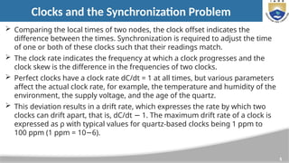
 Comparing the local times of two nodes, the clock offset indicates the
difference between the times. Synchronization is required to adjust the time
of one or both of these clocks such that their readings match.
 The clock rate indicates the frequency at which a clock progresses and the
clock skew is the difference in the frequencies of two clocks.
 Perfect clocks have a clock rate dC/dt = 1 at all times, but various parameters
affect the actual clock rate, for example, the temperature and humidity of the
environment, the supply voltage, and the age of the quartz.
 This deviation results in a drift rate, which expresses the rate by which two
clocks can drift apart, that is, dC/dt 1. The maximum drift rate of a clock is
−
expressed as ρ with typical values for quartz-based clocks being 1 ppm to
100 ppm (1 ppm = 10 6).
−

6
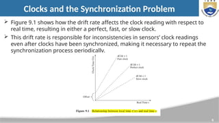
 Figure 9.1 shows how the drift rate affects the clock reading with respect to
real time, resulting in either a perfect, fast, or slow clock.
 This drift rate is responsible for inconsistencies in sensors’ clock readings
even after clocks have been synchronized, making it necessary to repeat the
synchronization process periodically.

7
Time Synchronization in Wireless Sensor Networks
 Time synchronization is a required service for many applications and services in
distributed systems in general.
 Numerous protocols for time synchronization have been proposed for both wired
and wireless systems, for example, the Network Time Protocol (NTP) is a widely
deployed, scalable, robust, and self-configurable synchronization approach.
 Particularly in combination with the Global Positioning System (GPS), it has been
shown to achieve accuracy in the order of a few microseconds.
 However, approaches such as NTP are not suitable for WSNs due to these
networks’ unique characteristics and constraints.

8
Reasons for Time Synchronization
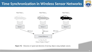
 Sensors in a WSN monitor objects in the physical world and report activities and
events to interested observers.
 For example, proximity detecting sensors, such as magnetic, capacitive, or acoustic
sensors, trigger an event when a moving object (e.g., a car) passes (see Figure
9.2).
 In dense sensor networks, multiple sensors will observe the same activity and
trigger such events.
 Accurate temporal correlation of these events is crucial to answer questions such as
How many moving objects have been detected?, What is the direction of the moving
object?, and What is the speed of the moving object?
 As a consequence, it is important that an observer can establish the correct logical
order of events;

9

10
 Time synchronization is also necessary for a variety of applications and algorithms
in distributed systems in general, including communication protocols (e.g., at-most-
once message delivery), security, data consistency and concurrency control.
 With respect to energy, many WSNs rely on sleep/wake protocols that allow a
network switch off sensor nodes or let them enter low-power sleep modes.
 Localization in WSNs is necessary to correctly position sensors or the objects they
monitor. Many localization techniques rely on ranging technologies to estimate
distances between nodes and synchronization is required for time-of-flight
measurements of radio or acoustic signals.

11
Challenges for Time Synchronization
 Traditional time synchronization protocols have been designed for use in wired
networks and do not consider the challenges inherit to low-cost low-power sensor
nodes and the wireless medium.
 Similar to wired environments, time synchronization in WSNs is exposed to
challenges such as clock glitches and varying clock drifts due to changes in
temperature and humidity.
 However, time synchronization protocols for sensor networks must consider an array
of additional challenges and constraints such as:
• Environmental Effects
• Energy Constraints
• Wireless Medium and Mobility
• Additional Constraints

12
Basics of Time Synchronization
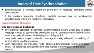
 Synchronization is typically based on some sort of message exchange among
sensor nodes.
 If the medium supports broadcast, multiple devices can be synchronized
simultaneously with a low number of messages.
Synchronization Messages
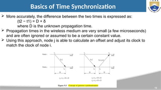
One-Way Message Exchange
 The simplest approach of pairwise synchronization occurs when only a single
message is used to synchronize two nodes, that is, one node sends a time stamp
to another node, illustrated in the left graph of Figure 9.3.
 Here, node i sends a synchronization message to node j at time t1, embedding t1
as time stamp into the message.
 Upon reception of this message, node j obtains a time stamp t2 from its own local
clock. The difference between the two time stamps is an indicator of the clock
offset δ.

13
 More accurately, the difference between the two times is expressed as:
(t2 − t1) = D + δ
where D is the unknown propagation time.
 Propagation times in the wireless medium are very small (a few microseconds)
and are often ignored or assumed to be a certain constant value.
 Using this approach, node j is able to calculate an offset and adjust its clock to
match the clock of node i.

14
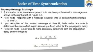
Two-Way Message Exchange
 A somewhat more accurate approach is to use two synchronization messages as
shown in the right graph of Figure 9.3.
 Here, node j responds with a message issued at time t3, containing time stamps
t1, t2, and t3.
 Upon reception of this second message at time t4, both nodes are able to
determine the clock offset, again assuming a fixed value for the propagation delay.
 However, node i is now able to more accurately determine both the propagation
delay and the offset as

15
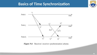
Receiver–Receiver Synchronization
 A different approach is taken by protocols that apply the receiver–receiver
synchronization principle, where synchronization is based on the time at which the
same message arrives at each receiver.
 This is in contrast to the more traditional sender–receiver approach of most
synchronization schemes.
 In broadcast environments, these receivers obtain the message at about the
same time and then exchange their arrival times to compute an offset (i.e., the
difference in reception times indicates the offset of their clocks).
 Figure 9.4 shows an example of this scheme. If there are two receivers, three
messages are needed to synchronize both receivers.

16

17
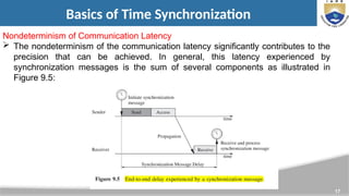
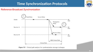
Nondeterminism of Communication Latency
 The nondeterminism of the communication latency significantly contributes to the
precision that can be achieved. In general, this latency experienced by
synchronization messages is the sum of several components as illustrated in
Figure 9.5:

18
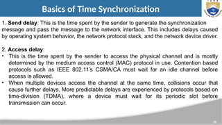
1. Send delay: This is the time spent by the sender to generate the synchronization
message and pass the message to the network interface. This includes delays caused
by operating system behavior, the network protocol stack, and the network device driver.
2. Access delay:
• This is the time spent by the sender to access the physical channel and is mostly
determined by the medium access control (MAC) protocol in use. Contention based
protocols such as IEEE 802.11’s CSMA/CA must wait for an idle channel before
access is allowed.
• When multiple devices access the channel at the same time, collisions occur that
cause further delays. More predictable delays are experienced by protocols based on
time-division (TDMA), where a device must wait for its periodic slot before
transmission can occur.

19
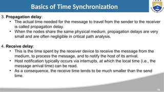
3. Propagation delay:
• The actual time needed for the message to travel from the sender to the receiver
is called propagation delay.
• When the nodes share the same physical medium, propagation delays are very
small and are often negligible in critical path analysis.
4. Receive delay:
• This is the time spent by the receiver device to receive the message from the
medium, to process the message, and to notify the host of its arrival.
• Host notification typically occurs via interrupts, at which the local time (i.e., the
message arrival time) can be read.
• As a consequence, the receive time tends to be much smaller than the send
time.

20
Time Synchronization Protocols
 Numerous time synchronization protocols for WSNs have been developed, where
most of them are based on some variations of the message exchange concepts.
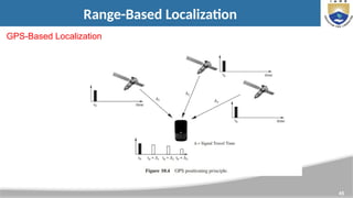
Reference Broadcasts Using Global Sources of Time
 The Global Positioning System (GPS) continuously broadcasts time measured
from an epoch started at 0h 6 January, 1980 UTC. However, unlike UTC, GPS is
not perturbed by leap seconds and is therefore ahead of UTC by an integer
number of seconds (15 seconds as of 2009).
 Even inexpensive GPS receivers can receive GPS time with a precision of 200
ns. Time signals are also being transmitted by terrestrial radio stations.
 However, such approaches exhibit a number of challenges that prohibit their use
for many WSNs.
 Many sensor networks are hierarchical systems consisting of low-power sensor
devices, but also more powerful devices that often serve as gateways or cluster
heads.

21
Lightweight Tree-Based Synchronization
 The primary goal of the Lightweight Tree-Based Synchronization (LTS) protocol
is to provide a specified precision (instead of a maximum precision) with as little
overhead as possible.
 LTS can be used with different algorithms for both centralized and decentralized
multi-hop synchronization.
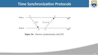
 To understand the approach taken by LTS, let us first consider the message
exchange for the synchronization of a pair of nodes. Figure 9.6 shows a graphical
depiction of this scheme.

22

23
Timing-sync Protocol for Sensor Networks
 The Timing-sync Protocol for Sensor Networks (TPSN) is another traditional
sender–receiver synchronization approach that uses a tree to organize a
network.
 TPSN uses two phases for synchronization:
• the level discovery phase (executed during network deployment) and
• the synchronization phase.

24
Flooding Time Synchronization Protocol
 The goals of the Flooding Time Synchronization Protocol (FTSP) are to achieve
network-wide synchronization with errors in the microsecond range, scalability up
to hundreds of nodes, and robustness to changes in network topology including
link and node failures.
 FTSP differs from other solutions in that it uses a single broadcast to establish
synchronization points between sender and receivers while eliminating most
sources of synchronization error.
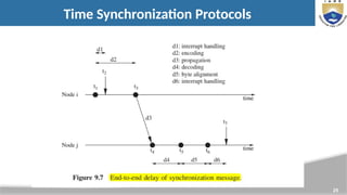
 Toward this end, FTSP expands on the delay analysis and decomposes the end-
to-end delay into the components shown in Figure 9.7.

25

26
Time-Stamping in FTSP
 In FTSP, a sender synchronizes one or more receivers with a single radio
broadcast, where the broadcast message contains the sender’s time stamp.
 Upon arrival, a receiver extracts the time stamp from the message and time
stamps the arrival using its own local clock.
 The global–local time pair provides a synchronization point. The sender’s time
stamp must be embedded into the currently transmitted message, therefore the
time stamping must occur before the bytes containing the time stamp are
transmitted over the medium.
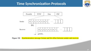
 In FTSP, the synchronization message begins with a number of preamble bytes
followed by several SYNC bytes, a data field, and a cyclic redundancy check
(CRC) for error detection (Figure 9.8).

27

28
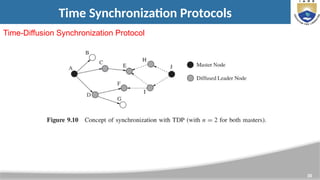
Multi-Hop Synchronization
 Similar to TPSN, FTSP relies on an elected synchronization root to synchronize
the network, where root election is based on unique node IDs.
 The root node maintains the global time and all other nodes in the network
synchronize their clocks to that of the root. Synchronization is triggered through a
broadcast message by the root node containing its time stamp.
 All nodes within the communication range of the root can establish
synchronization points directly from the broadcast message.
 Other nodes collect synchronization points from broadcasts of synchronized
nodes that are closer to the root.

29
Reference-Broadcast Synchronization

30
Time-Diffusion Synchronization Protocol

31
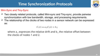
Mini-Sync and Tiny-Sync
 Two closely related protocols, called Mini-sync and Tiny-sync, provide pairwise
synchronization with low bandwidth, storage, and processing requirements.
 The relationship of the clocks of two nodes in a sensor network can be expressed
as:
where a12 expresses the relative drift and b12 the relative offset between
the clocks of nodes 1 and 2.

32
Localization
 Localization is the task of determining the physical coordinates of a sensor node (or
a group of sensor nodes) or the spatial relationships among objects.
 It comprises a set of techniques and mechanisms that allow a sensor to estimate its
own location based on information gathered from the sensor’s environment.
 While the Global Positioning System (GPS) is undoubtedly the most well-known
location-sensing system, it is not accessible in all environments (e.g., indoors or
under dense foliage) and may incur resource costs unacceptable for resource-
constrained wireless sensor networks (WSNs).
 Localization is fundamental for sensor network services that rely on the knowledge
of sensor positions, including geographic routing and coverage area management.

33
Localization
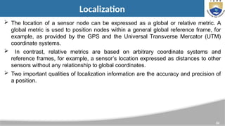
 The location of a sensor node can be expressed as a global or relative metric. A
global metric is used to position nodes within a general global reference frame, for
example, as provided by the GPS and the Universal Transverse Mercator (UTM)
coordinate systems.
 In contrast, relative metrics are based on arbitrary coordinate systems and
reference frames, for example, a sensor’s location expressed as distances to other
sensors without any relationship to global coordinates.
 Two important qualities of localization information are the accuracy and precision of
a position.

34
Localization
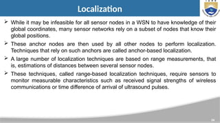
 While it may be infeasible for all sensor nodes in a WSN to have knowledge of their
global coordinates, many sensor networks rely on a subset of nodes that know their
global positions.
 These anchor nodes are then used by all other nodes to perform localization.
Techniques that rely on such anchors are called anchor-based localization.
 A large number of localization techniques are based on range measurements, that
is, estimations of distances between several sensor nodes.
 These techniques, called range-based localization techniques, require sensors to
monitor measurable characteristics such as received signal strengths of wireless
communications or time difference of arrival of ultrasound pulses.

35
Ranging Techniques
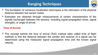
 The foundation of numerous localization techniques is the estimation of the physical
distance between two sensor nodes.
 Estimates are obtained through measurements of certain characteristics of the
signals exchanged between the sensors, including signal propagation times, signal
strengths, or angle of arrival.
 The concept behind the time of arrival (ToA) method (also called time of flight
method) is that the distance between the sender and receiver of a signal can be
determined using the measured signal propagation time and the known signal
velocity.
Time of Arrival

36
Ranging Techniques
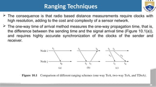
 The consequence is that radio based distance measurements require clocks with
high resolution, adding to the cost and complexity of a sensor network.
 The one-way time of arrival method measures the one-way propagation time, that is,
the difference between the sending time and the signal arrival time (Figure 10.1(a)),
and requires highly accurate synchronization of the clocks of the sender and
receiver.

37
Ranging Techniques
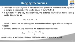
 Therefore, the two-way time of arrival method is preferred, where the round-trip time
of a signal is measured at the sender device (Figure 10.1(b)).
 In summary, for one-way measurements, the distance between two nodes i and j
can be determined as:
where t1 and t2 are the sending and receive times of the signal and v is the signal
velocity.
 Similarly, for the two-way approach, the distance is calculated as:
where t3 and t4 are the sending and receive times of the response signal.

38
Ranging Techniques
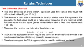
Time Difference of Arrival
 The time difference of arrival (TDoA) approach uses two signals that travel with
different velocities (Figure 10.1(c)).
 The receiver is then able to determine its location similar to the ToA approach. For
example, the first signal could be a radio signal (issued at t1 and received at t2),
followed by an acoustic signal (either immediately or after a fixed time interval twait
= t3 − t1).
 Therefore, the receiver can determine the distance as:
 TDoA-based approaches do not require the clocks of the sender and receiver to be
synchronized and can obtain very accurate measurements.
 The disadvantage of the TDoA approach is the need for additional hardware.

39
Ranging Techniques
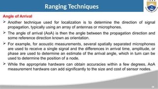
Angle of Arrival
 Another technique used for localization is to determine the direction of signal
propagation, typically using an array of antennas or microphones.
 The angle of arrival (AoA) is then the angle between the propagation direction and
some reference direction known as orientation.
 For example, for acoustic measurements, several spatially separated microphones
are used to receive a single signal and the differences in arrival time, amplitude, or
phase are used to determine an estimate of the arrival angle, which in turn can be
used to determine the position of a node.
 While the appropriate hardware can obtain accuracies within a few degrees, AoA
measurement hardware can add significantly to the size and cost of sensor nodes.

40
Ranging Techniques
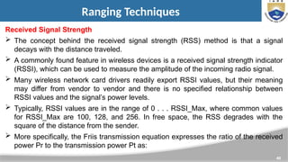
Received Signal Strength
 The concept behind the received signal strength (RSS) method is that a signal
decays with the distance traveled.
 A commonly found feature in wireless devices is a received signal strength indicator
(RSSI), which can be used to measure the amplitude of the incoming radio signal.
 Many wireless network card drivers readily export RSSI values, but their meaning
may differ from vendor to vendor and there is no specified relationship between
RSSI values and the signal’s power levels.
 Typically, RSSI values are in the range of 0 . . . RSSI_Max, where common values
for RSSI_Max are 100, 128, and 256. In free space, the RSS degrades with the
square of the distance from the sender.
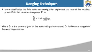
 More specifically, the Friis transmission equation expresses the ratio of the received
power Pr to the transmission power Pt as:

41
Ranging Techniques
 More specifically, the Friis transmission equation expresses the ratio of the received
power Pr to the transmission power Pt as:
where Gt is the antenna gain of the transmitting antenna and Gr is the antenna gain of
the receiving antenna.

42
Range-Based Localization
Triangulation
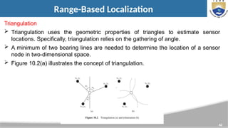
 Triangulation uses the geometric properties of triangles to estimate sensor
locations. Specifically, triangulation relies on the gathering of angle.
 A minimum of two bearing lines are needed to determine the location of a sensor
node in two-dimensional space.
 Figure 10.2(a) illustrates the concept of triangulation.

43
Trilateration
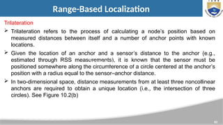
 Trilateration refers to the process of calculating a node’s position based on
measured distances between itself and a number of anchor points with known
locations.
 Given the location of an anchor and a sensor’s distance to the anchor (e.g.,
estimated through RSS measurements), it is known that the sensor must be
positioned somewhere along the circumference of a circle centered at the anchor’s
position with a radius equal to the sensor–anchor distance.
 In two-dimensional space, distance measurements from at least three noncollinear
anchors are required to obtain a unique location (i.e., the intersection of three
circles). See Figure 10.2(b)
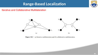
Iterative and Collaborative Multilateration

44
Iterative and Collaborative Multilateration

45
GPS-Based Localization

46
Range-Free Localization
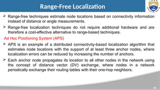
 Range-free techniques estimate node locations based on connectivity information
instead of distance or angle measurements.
 Range-free localization techniques do not require additional hardware and are
therefore a cost-effective alternative to range-based techniques.
Ad Hoc Positioning System (APS)
 APS is an example of a distributed connectivity-based localization algorithm that
estimates node locations with the support of at least three anchor nodes, where
localization errors can be reduced by increasing the number of anchors.
 Each anchor node propagates its location to all other nodes in the network using
the concept of distance vector (DV) exchange, where nodes in a network
periodically exchange their routing tables with their one-hop neighbors.

47
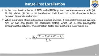
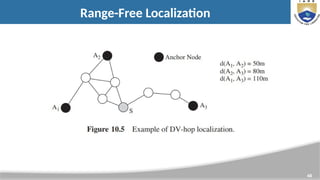
 In the most basic scheme of APS, called DV-hop, each node maintains a table {Xi,
Yi, hi}, where {Xi, Yi} is the location of node I and hi is the distance in hops
between this node and node i.
 When an anchor obtains distances to other anchors, it then determines an average
size for one hop (called the correction factor), which too is then propagated
throughout the network. The correction factor ci of anchor i is determined as:

49
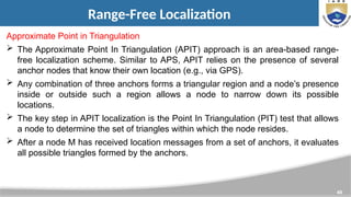
Approximate Point in Triangulation
 The Approximate Point In Triangulation (APIT) approach is an area-based range-
free localization scheme. Similar to APS, APIT relies on the presence of several
anchor nodes that know their own location (e.g., via GPS).
 Any combination of three anchors forms a triangular region and a node’s presence
inside or outside such a region allows a node to narrow down its possible
locations.
 The key step in APIT localization is the Point In Triangulation (PIT) test that allows
a node to determine the set of triangles within which the node resides.
 After a node M has received location messages from a set of anchors, it evaluates
all possible triangles formed by the anchors.

50
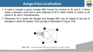
 A node is outside a given triangle ABC formed by anchors A, B, and C, if there
exists a direction such that a point adjacent to M is either further or closer to all
points A, B, and C simultaneously.
 Otherwise, M is inside the triangle and triangle ABC can be added to the set of
triangles in which M resides. This concept is illustrated in Figure 10.6.

51
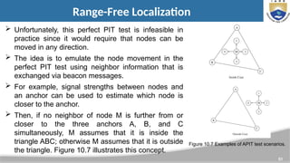
 Unfortunately, this perfect PIT test is infeasible in
practice since it would require that nodes can be
moved in any direction.
 The idea is to emulate the node movement in the
perfect PIT test using neighbor information that is
exchanged via beacon messages.
 For example, signal strengths between nodes and
an anchor can be used to estimate which node is
closer to the anchor.
 Then, if no neighbor of node M is further from or
closer to the three anchors A, B, and C
simultaneously, M assumes that it is inside the
triangle ABC; otherwise M assumes that it is outside
the triangle. Figure 10.7 illustrates this concept.
Figure 10.7 Examples of APIT test scenarios.

52
Localization Based on Multidimensional Scaling
 Multidimensional scaling (MDS) has its roots in psychometrics and psychophysics
and is a set of data analysis techniques that display the structure of distance-like
data as a geometrical picture.
 Applied to localization, MDS can be used in centralized localization techniques,
where a powerful central device collects information from the network, determines
the nodes’ locations, and propagates this information back into the network.
 The network is represented as an undirected graph of n nodes (m<n of which are
anchors and know their locations) and edges representing the connectivity
information.
 Given the distances between all pairs of nodes, the goal of MDS is to preserve the
distance information such that the network can be recreated in the multidimensional
space. The result of MDS will be an arbitrarily rotated and flipped version of the
original network layout.

53
Event-Driven Localization
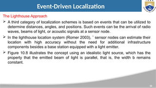
The Lighthouse Approach
 A third category of localization schemes is based on events that can be utilized to
determine distances, angles, and positions. Such events can be the arrival of radio
waves, beams of light, or acoustic signals at a sensor node.
 In the lighthouse location system (Romer 2003), ¨ sensor nodes can estimate their
location with high accuracy without the need for additional infrastructure
components besides a base station equipped with a light emitter.
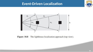
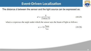
 Figure 10.8 illustrates the concept using an idealistic light source, which has the
property that the emitted beam of light is parallel, that is, the width b remains
constant.

55
The distance d between the sensor and the light source can be expressed as:

56
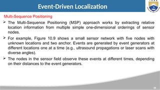
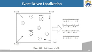
Multi-Sequence Positioning
 The Multi-Sequence Positioning (MSP) approach works by extracting relative
location information from multiple simple one-dimensional orderings of sensor
nodes.
 For example, Figure 10.9 shows a small sensor network with five nodes with
unknown locations and two anchor. Events are generated by event generators at
different locations one at a time (e.g., ultrasound propagations or laser scans with
diverse angles).
 The nodes in the sensor field observe these events at different times, depending
on their distances to the event generators.

57
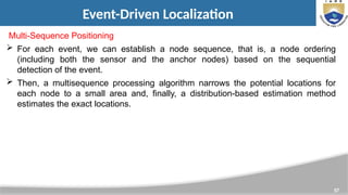
Multi-Sequence Positioning
 For each event, we can establish a node sequence, that is, a node ordering
(including both the sensor and the anchor nodes) based on the sequential
detection of the event.
 Then, a multisequence processing algorithm narrows the potential locations for
each node to a small area and, finally, a distribution-based estimation method
estimates the exact locations.

time synchronization and localization .pptx

More Related Content

Similar to time synchronization and localization .pptx

More from 22951a04p3

Recently uploaded

time synchronization and localization .pptx