Here is a detailed **SlideShare description (approx. 3000 words)** for your uploaded presentation **“Time\_Complexity\_Goodrich.pptx”**, based on the book *Data Structures and Algorithms in Python* by **Michael T. Goodrich, Roberto Tamassia, and David Mount**. --- ## 📘 **SlideShare Description: Time Complexity – A Complete Guide Based on Goodrich, Tamassia & Mount** --- ### **🎓 Overview** This SlideShare presentation offers a deep dive into the concept of **Time Complexity** in computer science, as introduced in the textbook *Data Structures and Algorithms in Python* by **Goodrich, Tamassia, and Mount**. It explains how to analyze the efficiency of algorithms by understanding how their runtime increases with input size, and is ideal for students, educators, developers, and professionals preparing for technical interviews. 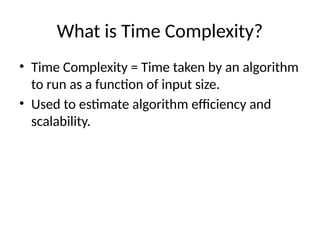--- ## 🔍 **What is Time Complexity?** Time complexity is a **mathematical representation of how the running time of an algorithm grows with the size of the input (n)**. It’s used to evaluate algorithm performance in a system-independent way. Unlike actual running time, which can vary with hardware or language, time complexity gives a generalized, theoretical estimate. 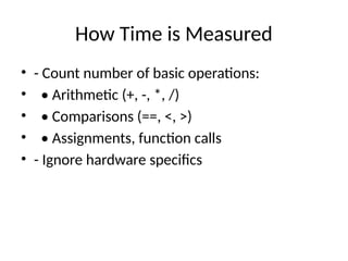--- ### **Formal Definition** **Time Complexity** of an algorithm = Number of basic operations executed as a function of input size `n`. 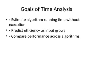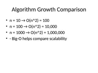These operations can include: * Arithmetic operations (`+`, `-`, `*`, `/`) * Comparisons (`==`, `<`, `>`) * Assignments (`=`) * Function calls or returns * Data access or traversal steps --- ### **Why Analyze Time Complexity?** * To **predict performance** without executing code * To **compare multiple algorithms** * To **determine scalability** * To **avoid inefficient solutions** as data grows * To **choose suitable algorithms** in real-world applications (e.g., search engines, big data, AI) --- ## ⏳ **Measuring Time Complexity** Time complexity is usually estimated by: 1. Counting the **number of operations** 2. Ignoring **machine-dependent factors** 3. Focusing on the **dominant term** as `n → ∞` This leads to the use of **asymptotic notation**, which describes behavior for large input sizes. 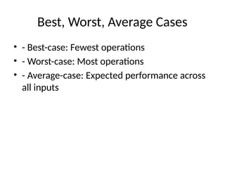--- ## 🔢 **Asymptotic Notations** ### **Big-O Notation (O)** Describes the **worst-case** upper bound. ### **Big-Omega (Ω)** Describes the **best-case** lower bound. ### **Theta (Θ)** Describes the **tight bound** (average-case for some cases). 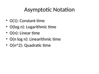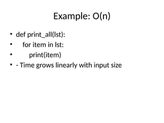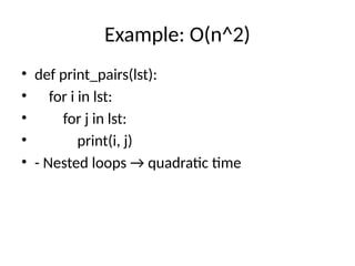--- ### **Common Big-O Complexities** | Complexity | Name | Example Use Case | | ---------- | ------------ | ------------------------------------- | | O(1) | Constant | Accessing an array element | | O(log n) | Logarithmic | Binary Search | | O(n) | Linear | Iterating through an array | | O(n log n) | Linearithmic | Merge Sort, Quick Sort (average case) | | O(n²) | Quadratic | Bubble Sort, Insertion Sort | | O(2ⁿ) | Exponential | Recursive F

1. Time Complexity
Based on Goodrich, Tamassia, Mount
- DS&A in Python
Department of Computer Science

2. What is Time Complexity?
• Time Complexity = Time taken by an algorithm
to run as a function of input size.
• Used to estimate algorithm efficiency and
scalability.

3. Goals of Time Analysis
• - Estimate algorithm running time without
execution
• - Predict efficiency as input grows
• - Compare performance across algorithms

4. How Time is Measured
• - Count number of basic operations:
• • Arithmetic (+, -, *, /)
• • Comparisons (==, <, >)
• • Assignments, function calls
• - Ignore hardware specifics

5. Asymptotic Notation
• O(1): Constant time
• O(log n): Logarithmic time
• O(n): Linear time
• O(n log n): Linearithmic time
• O(n^2): Quadratic time

6. Example: O(1)
• def get_first(lst):
• return lst[0]
• - Always takes same time regardless of list size

7. Example: O(n)
• def print_all(lst):
• for item in lst:
• print(item)
• - Time grows linearly with input size

8. Example: O(n^2)
• def print_pairs(lst):
• for i in lst:
• for j in lst:
• print(i, j)
• - Nested loops → quadratic time

9. Best, Worst, Average Cases
• - Best-case: Fewest operations
• - Worst-case: Most operations
• - Average-case: Expected performance across
all inputs

10. Algorithm Growth Comparison
• n = 10 → O(n^2) = 100
• n = 100 → O(n^2) = 10,000
• n = 1000 → O(n^2) = 1,000,000
• - Big-O helps compare scalability

11. Time vs Space Trade-Off
• - Use more memory to reduce time
• - Example: Memoization (store results to save
computation)

12. Best Practices
• - Minimize nested loops
• - Use efficient data structures (e.g., sets)
• - Avoid repeated work via
caching/precomputation