The document summarizes Robert Murtagh's PhD thesis on analytical models of single bubbles and foams. It includes a declaration of authorship, acknowledgements, and a summary of the thesis contents. The thesis uses a "Z-cone model" to model bubbles as collections of circular cones joined at their bases. It applies this model to study the energy of ordered foams and the bubble-bubble interaction over a range of liquid fractions. It also adapts the model to study the energy of a Kelvin foam cell and investigates contact losses in the Kelvin structure away from the wet limit. Finally, it examines the evolution of gas bubbles on a liquid surface containing mixtures of gases with different solubilities.


![List of Figures xii
7.4 Comparison of the excess energy of large and small bubbles from
the curved cone model with the Surface Evolver. . . . . . . . . . . . 104
7.5 Excess energies ε and ε/ξ2
for large and small bubbles in a simple
cubic arrangement for a = 1.5. . . . . . . . . . . . . . . . . . . . . . 105
7.6 Variation of the excess energy for a range of polydispersities. . . . . 107
7.7 The radius of the contact line (upper) and of the film (lower) sepa-
rating two bubbles in a two-bubble cluster. . . . . . . . . . . . . . . 109
7.8 Variation of excess energy with distance between bubble centres for
the two-bubble chain. . . . . . . . . . . . . . . . . . . . . . . . . . . 109
A.1 Dividing up a spherical bubble in the Z-cone model. . . . . . . . . . 111
C.1 Sketch of the concavity of the surface of a large bubble due to a
curved contact. . . . . . . . . . . . . . . . . . . . . . . . . . . . . . 126
D.1 Cross-section of a square cone in the Kelvin cone model with Vi
and V ∗
i shown. . . . . . . . . . . . . . . . . . . . . . . . . . . . . . 137
E.1 Sketch of surface tension forces acting at an edge between a quadri-
lateral face and two hexagons. . . . . . . . . . . . . . . . . . . . . . 141
F.1 Equilibrium structure for a conventional cell in a Kelvin foam, from
the Surface Evolver. . . . . . . . . . . . . . . . . . . . . . . . . . . 145
G.1 Schematic 2-D cross-section of a gas bubble (Phase 1) at the surface
of a liquid (Phase 2), reproduced from [57]. . . . . . . . . . . . . . . 147](https://image.slidesharecdn.com/0b1eb23b-c092-4b30-8aa1-2e454aa93edb-160425224409/85/Thesis_Robert_Murtagh_Corrected-13-320.jpg)

![Chapter 1
General Introduction
1.1 Introduction
Although usually going unnoticed, foams are an indispensable part of modern
society. The student of foams cannot help but be reminded of the impacts of
the physics of foam on the world today. From the industrial process of mineral
flotation [1], in which foam is used to separate valuable minerals such as copper
and lead from their native ores by harnessing a difference in hydrophobicities (or
affinity for water), to more routine shaving foam and the head of a cappuccino.
Despite there being a presumed knowledge of what is and is not a foam, given
the wide range of observed physical properties and different applications, it then
becomes necessary to clarify; “what exactly is a foam?”
A liquid foam is a two-phase system in which gas bubbles are dispersed in a con-
tinuous liquid phase [2, 3]. The gas phase is often present in large quantities
leading to the common understanding of a foam as a collection of gas bubbles
separated by continuous liquid films. Foams often exhibit similar physical prop-
erties to emulsions, which are made up of a continuous liquid phase with a liquid
dispersed phase [4–7].
1](https://image.slidesharecdn.com/0b1eb23b-c092-4b30-8aa1-2e454aa93edb-160425224409/85/Thesis_Robert_Murtagh_Corrected-15-320.jpg)
![Chapter 1. General Introduction 2
The liquid fraction φ of a foam (hereafter “foam” will be used to refer to emul-
sions as well as liquid foams for simplicity) is defined as the ratio of the volume
of the continuous liquid phase to the total volume of the foam [2]. A foam with a
very high liquid fraction φ is naturally referred to as a “wet” foam while a foam
with a very low liquid fraction φ is referred to as a “dry” foam. Examples of wet
and dry foams are shown in Figure 1.1.
However, most foams that we encounter have a liquid fraction somewhere between
these two extremes and it is not altogether clear, theoretically, what liquid fraction
demarcates a “wet” foam from a “dry” foam. As shown in Figure 1.1, a dry foam
is characterised by polyhedral bubbles which arrange in such a way as to satisfy
Plateau’s rules (see Section 1.2) while wet foam bubbles are rounded, tending to
resemble a packing of spheres for high liquid fractions. In practical terms, a liquid
fraction of between 15% and 18% is often taken as the boundary between wet and
dry foams; a liquid fraction in this range is roughly halfway between 0% liquid
fraction, which denotes the so-called dry limit, and 36% liquid fraction, which is
called the wet limit or jamming transition above which the bubbles become
separated and no longer constitute a foam [8, 9]. We will discuss the nature of the
jamming transition further in Section 1.3. This distinction is not important for
the arguments presented in this thesis as we will focus mostly on very wet foams.
However, merely specifying a single factor of a foam, such as an average liquid
fraction, is not sufficient to fully describe a foam. For example, while the average
liquid fraction helps to generally identify whether a foam is wet or dry, the local
liquid fraction will be higher close to the liquid pool and much lower at the top
of the foam as liquid drains under gravity, as we can clearly see from Figure 1.1.
Drainage of the liquid over time gives rise to a height profile for the liquid fraction
which is not captured by the average liquid fraction (see Section 1.5).
The study of foams is usually split into four areas.
1. Structure is concerned with the geometry of soap bubbles that have been
packed together, usually in the bulk of a foam.](https://image.slidesharecdn.com/0b1eb23b-c092-4b30-8aa1-2e454aa93edb-160425224409/85/Thesis_Robert_Murtagh_Corrected-16-320.jpg)

![Chapter 1. General Introduction 4
2. Drainage relates to the motion of liquid through the channels within a
foam, due to the force of gravity.
3. Coarsening refers to the diffusion of gas between bubbles within a foam,
with the general consequence that large bubbles get larger and small bubbles
get smaller.
4. Rheology is the study of the deformation and flow of foam in response to
an applied stress.
For the most part, we will concern ourselves with foam structure, although we will
discuss coarsening in Chapter 6.
1.2 Plateau’s Rules for Dry Foams
The structure of foams in both the wet and dry limits is a very active area of
research. In the limit of a “dry” foam (i.e as φ → 0) the bubbles become deformed
(see Figure 1.1(b)). The very small amount of liquid left in the foam is distributed
between the soap films which separate the polyhedra.
The first description of the equilibrium structure of a dry foam was given by
Joseph Plateau in his 1873 book “Statique Exp´erimentale et Th´eorique des Liq-
uides soumis aux seules Forces Mol´ecularies” [10] and it contains a set of empirical
laws (known as Plateau’s Rules) which are obeyed by the thin (liquid) films sep-
arating the bubbles in a dry foam. Namely,
1. Thin films can only meet three at a time forming a Plateau border. The
angle between the films must be 2π
3
radians.
2. No more than four Plateau borders may meet at a vertex. The angle be-
tween the Plateau borders at this vertex is the regular tetrahedral angle of
arccos(−1/3) radians (≈ 109.47◦
). This condition also limits the number of
films meeting at a vertex to six.](https://image.slidesharecdn.com/0b1eb23b-c092-4b30-8aa1-2e454aa93edb-160425224409/85/Thesis_Robert_Murtagh_Corrected-18-320.jpg)
![Chapter 1. General Introduction 5
3. Each thin film must have a constant mean curvature related to the Laplace
pressure difference ∆P across the thin film, according to the Young-Laplace
law [2, 3],
∆P =
2σ
Rc
(1.1)
where σ is the surface tension and Rc is the mean radius of curvature of
the film, which is constant. The Laplace pressure for a bubble (two films),
rather than a single film, is simply 4σ/R0 where R0 is the bubble radius.
Despite being known for over a hundred years, the theoretical proof of Plateau’s
laws was only provided in 1976 by Jean Taylor [11].
With increasing liquid fraction of the foam (above ∼ 2% [2]), the Plateau borders
and vertices swell, forming a liquid network in the foam for which Plateau’s law
no longer strictly apply.
1.3 The Wet Limit
The bubbles in a foam with a very high liquid fraction are no longer polyhedral,
being better described as “more or less” spherical and the structure of such a foam
can be thought of as a dense packing of spheres. The wet limit is defined as the
point at which the bubbles are spheres and have only point contacts with each of
their neighbouring bubbles. In Section 1.1, we referred to this as the wet limit or
the jamming transition.
The liquid fraction at which this occurs is called the “critical liquid fraction” φc
and is approximately 0.36 in three dimensions for a random-close-packing (RCP)
of spheres [8]. At RCP, the interaction between neighbouring bubbles is strong
enough to give stability and rigidity to the collection of bubbles forming a foam,
while for higher liquid fractions the bubbles separate from each other to form a
bubbly liquid.](https://image.slidesharecdn.com/0b1eb23b-c092-4b30-8aa1-2e454aa93edb-160425224409/85/Thesis_Robert_Murtagh_Corrected-19-320.jpg)
![Chapter 1. General Introduction 6
(a) (b)
Figure 1.2: (a) The face-centred cubic (fcc) and (b) body-centred cubic (bcc)
lattices. The critical liquid fraction associated with these structures are φc =
0.26 and φc ≈ 0.32, respectively. Both of these structures are of relevance in
monodisperse foam studies [12] and will be discussed later in this thesis with
regard to the cone model (see Chapters 2, 4 and 5).
It should be noted that the value φc is different if the bubble positions are not
random but are ordered, for example as a crystal lattice. For the fcc crystal lattice,
shown in Figure 1.2(a), φc = 0.26 while for the bcc crystal shown in Figure 1.2(b)
φc = 1 −
√
3π
8
≈ 0.32. The fascinating subject of ordered foam structures will be
discussed in greater detail in Chapter 2 in the context of the Z-cone model.
1.4 Monodisperse Foam Structures
When discussing ordering in foams, an important parameter to consider is the
bubble size. For much of this work, the most convenient measure of bubble size is
the equivalent sphere radius which we denote by R0. It is defined by
R0 =
3 3V
4π
. (1.2)
While disordered structures may be formed by foams with a wide size distribution
or polydispersity [2], many of the most interesting ordered structures arise in
monodisperse foams, in which all of the bubbles have the same radius R0 [12]. Two](https://image.slidesharecdn.com/0b1eb23b-c092-4b30-8aa1-2e454aa93edb-160425224409/85/Thesis_Robert_Murtagh_Corrected-20-320.jpg)
![Chapter 1. General Introduction 7
such monodisperse structures, the Kelvin and Weaire-Phelan structures [13, 14],
are shown in Figure 1.3.
From an experimental standpoint, monodisperse foams can be made relatively
easily using a flow-focussing device [15, 16] and may also be made to crystallise
into well-defined ordered structures over time [17].
(a) (b)
Figure 1.3: (a) The double bubble unit cell of Kelvin’s tetrakaidecahedron
with curved faces, generated using the Surface Evolver [18]. (b) Experimental
image of the Weaire-Phelan structure courtesy of A. Meagher [14].
Theoretically, monodisperse foam is an often-used system in the study of pack-
ing. In fact, both experimental and theoretical approaches involving monodisperse
foams have been instrumental in attempts to answer a famous question in the study
of packings: which unit cell, infinitely repeated, partitions space into cells of equal
volume such that a minimal amount of surface area separates the cells?
Kelvin, in his treatise “On the Division of Space with Minimal Partition Area”
of 1887 [19], demonstrated using a combination of soap films on wire frames (a
common representation of a bubble in a monodisperse dry foam) and simple mathe-
matical arguments that a non-orthic truncated octahedron (or “Kelvin tetrakaidec-
ahedron”), shown in Figure 1.3 (a), had a lower surface area to volume ratio than
any of the Archimedean solids and many other common crystal structures. Sur-
prisingly, Kelvin never evaluated the energy of his proposed structure and, indeed,
this was not done until 100 years later [20]. The Kelvin tetrakaidecahedron has](https://image.slidesharecdn.com/0b1eb23b-c092-4b30-8aa1-2e454aa93edb-160425224409/85/Thesis_Robert_Murtagh_Corrected-21-320.jpg)
![Chapter 1. General Introduction 8
been observed experimentally in real monodisperse foams on a number of occa-
sions since 2000 [12, 21, 22]. In 1994, a unit cell structure with an even lower
surface area to volume ratio by approximately 0.3% was discovered using a nu-
merical approach by Denis Weaire and Robert Phelan [23]. The Weaire-Phelan
structure was first observed experimentally in monodisperse foam by Meagher et
al. in 2012 [14].
1.5 Osmotic Pressure
Figure 1.4: A schematic diagram illustrating the concept of osmotic pressure.
The application of an osmotic pressure Π forces liquid out of the foam, causing
the bubbles to come into closer contact, deforming their shape. This image is
taken from H¨ohler et al. [12].
Thus far, our discussion has been concerned with equilibrium foam structures
in the wet and dry limits. However, it is interesting to consider what happens
as we transition from one limit to the other. Say, from the wet to the dry limit,
corresponding to the extraction of liquid from the foam. As liquid leaves the foam,
the bubbles become deformed, increasing their surface area, and hence surface
energy. For a foam in equilibrium, there must be a force present to counter this
increase in surface energy. This force manifests itself in the form of the osmotic
pressure.](https://image.slidesharecdn.com/0b1eb23b-c092-4b30-8aa1-2e454aa93edb-160425224409/85/Thesis_Robert_Murtagh_Corrected-22-320.jpg)
![Chapter 1. General Introduction 9
The osmotic pressure of a foam Π can be thought of as the force per unit area on
a semi-permeable membrane placed at the interface of the foam and a liquid pool
which does not allow the gas to pass through it (see Figure 1.4). As liquid passes
through the membrane, the ratio of liquid to gas (i.e. the average liquid fraction
φ) decreases and the bubbles in the foam are forced into closer contact, deforming
them.
The osmotic pressure Π is formally defined by
Π = −σ
∂S
∂V Vg=const.
, (1.3)
where S is the total surface area of the bubbles, given by the sum of the individual
bubble surface areas Ai, within a confined volume V and σ is the surface tension
[24]. Note that this expression assumes that the gaseous phase is incompress-
ible due to the need to keep the total gas volume Vg constant when taking this
derivative. The limiting values of the osmotic pressure in the wet and dry limits
are
Π → 0 for φ → φc, (1.4)
and
Π → ∞ for φ → 0, (1.5)
respectively.
The osmotic pressure is a global property of a foam in the sense that it depends
on the total area S of the foam sample and the average liquid fraction φ. In
an idealised crystalline foam in which each of the bubbles has the same volume
(and hence equivalent sphere radius R0), and their local packing arrangements
are identical, the local osmotic pressure will be identical to the overall osmotic
pressure for the whole foam.](https://image.slidesharecdn.com/0b1eb23b-c092-4b30-8aa1-2e454aa93edb-160425224409/85/Thesis_Robert_Murtagh_Corrected-23-320.jpg)
![Chapter 1. General Introduction 10
From dimensional analysis, it is possible to show that the osmotic pressure scales
as the surface tension σ divided by the bubble radius R0 [5, 12]. Thus, it is
common to consider instead the reduced osmotic pressure Π = Π
σ
R0
[12]. As
we noted in Section 1.1, in real foams the liquid fraction varies as a function of
the height above the bottom of the foam x (see Section 3.3), also known as the
reduced height.
We can relate the change in reduced osmotic pressure Π to the local liquid fraction
φ(x) at a height x above the bottom of the foam, where it is in contact with a
liquid pool [12],
dΠ = (1 − φ(x))dx. (1.6)
Expressing the differentials in equation (1.6) as partial derivatives, we obtain a
differential equation for the local liquid fraction profile,
∂φ(˜x)
∂x
=
1 − φ(x)
∂Π
∂φ
(1.7)
where φ(0) = φc, the critical liquid fraction. We will consider this equation in our
discussion of the Z-cone model in Chapter 3.
1.6 Surface Energy and Minimisation
The surface energy E of a bubble in a foam is directly proportional to its surface
area A such that
E = σA (1.8)
with the constant of proportionality σ being the surface tension.
The Kelvin and Weaire-Phelan structures are sophisticated examples of a general
principle which determines the structure of a foam: in equilibrium, a foam will](https://image.slidesharecdn.com/0b1eb23b-c092-4b30-8aa1-2e454aa93edb-160425224409/85/Thesis_Robert_Murtagh_Corrected-24-320.jpg)
![Chapter 1. General Introduction 11
relax to the state of lowest surface energy to volume ratio for the given confinement
conditions. The simplest and most elegant example of this principle is for a free
soap bubble in air, which assumes a spherical shape [2].
In our work we are primarily concerned with the lowest surface energy configura-
tion of a bubble confined within the bulk of an ordered monodisperse foam. In
equilibrium, such a bubble has Z discrete regions of contact or faces with
neighbouring bubbles. In idealised descriptions of dry foams these correspond to
infinitesimally thin films covering the entire bubble surface [25] while at random
close pack, the contact areas go to zero and the structure consists of spherical
bubbles with point contacts.
As discussed in Section 1.5, traversing from the wet to the dry limit is achieved
through the application of an osmotic pressure [2, 12, 26] leading the bubble to
undergo a constant volume deformation.
This type of deformation is accompanied by an increase in surface energy, consis-
tent with equation (1.8). A convenient quantity to compute is the dimensionless
(relative) excess surface energy ε of a bubble,
ε ≡
E − E0
E0
(1.9)
where E0 = 4πσR2
0 is the surface energy of an undeformed spherical bubble of
the same volume with radius R0 and E is the bubble surface energy defined in
equation (1.8).
Similarly, the degree of deformation may be conveniently quantified via the di-
mensionless deformation ξ, defined as
ξ =
R0 − h
R0
(1.10)
where h is the distance between the bubble centre and a bubble face. The di-
mensionless deformation ξ is related to the liquid fraction φ via the expression
φ = 1 − 1−φc
(ξ−1)3 , where φc is the critical liquid fraction [27].](https://image.slidesharecdn.com/0b1eb23b-c092-4b30-8aa1-2e454aa93edb-160425224409/85/Thesis_Robert_Murtagh_Corrected-25-320.jpg)
![Chapter 1. General Introduction 12
We must stress here that the deformation ξ, as we have defined it in equation
(1.10), is valid for both monodisperse and polydisperse systems. With the defor-
mation being measured to the middle of the contact, it is the pressure difference
between the bubbles which is the key factor here. While the Weaire-Phelan struc-
ture (see Figure 1.3(b) in Section 1.4) is a famous example of a monodisperse foam
where the individual bubbles have different pressures [14, 23], it is more common
for differing internal pressures to arise in polydisperse foam. In the case of equal
pressures, the pressure difference across the contact is zero and the deformation is
the same for each bubble. This is not true when the bubbles are of different vol-
umes; the Laplace pressure (see Section 1.2), P = 4σ/R0, scales with the inverse
of the bubble radius R0 and so the smaller of the two bubbles will have a higher
Laplace pressure. The presence of a finite Laplace pressure across the contact
leads to a curved contact. Thus, R0 and h are different for the larger and smaller
bubbles meaning that the deformation ξ calculated using equation (1.10) will be
different. We will discuss this in Chapter 7.
Nonetheless for any given foam structure, the dependence of the dimensionless
excess surface energy ε on the dimensionless deformation ξ may be numerically
calculated using the Surface Evolver [18] (see Appendix F for details on the Surface
Evolver). However, the numerical approach fails to provide us with the in depth
physical description necessary to better understand foams. For example, while
the bubble-bubble interaction in two dimensions is well-described by a harmonic
force, this is not a good description in three dimensions, as we will see, meaning
that we cannot reduce this interaction to the sort of simple spring model which
pervades many fields of physics.
For this reason, recent research has focused on various simple models which at-
tempt to reproduce the key features of the exact numerical results and will be the
focus of the next chapters.](https://image.slidesharecdn.com/0b1eb23b-c092-4b30-8aa1-2e454aa93edb-160425224409/85/Thesis_Robert_Murtagh_Corrected-26-320.jpg)
![Chapter 1. General Introduction 13
1.7 Review of Previous Theoretical Studies of
the Bubble-Bubble Interaction
In this section, we will discuss some important models of the bubble-bubble inter-
action which directly motivate the Z-cone model that we will introduce in Chapter
2. The key feature of all of these models is that they are designed to describe a
wet foam consisting of nearly spherical (or circular in 2D) bubbles. Thus, they are
qualitatively distinct from models of polyhedral dry foams for which adherence to
Plateau’s laws (see Section 1.2) is a fundamental requirement [25].
In keeping with the tendency of physicists to study two-dimensional systems for
simplicity, before exploring the more complicated three-dimensional systems, we
will start our overview by looking at some key insights garnered in two dimensions.
1.7.1 Soft Disk Model and Lacasse in 2D
The so-called “soft” disk model (also known as the bubble model) refers to a simple
dynamic model for interacting bubbles which was introduced first by Durian [28],
and further developed by Langlois et al., for the purposes of studying the flow
behaviour of foams in two dimensions [29].
In this model, the bubbles in a wet foams are represented by a collection of disks.
Below the critical liquid fraction φc, the disks interact by overlapping, illustrated
in Figure 1.5 for bubbles of radii Ri, Rj, giving rise to the understanding of these
disks as “soft”. Each of the overlapping disks experiences two forces due to the
overlap; a simple elastic repulsion and a viscous dissipation force. It is interesting
to note that this bears some similarity to dissipative particle dynamics (DPD)
[30, 31], a molecular dynamics simulation technique for dynamic and rheological
properties of complex fluids. Similarly to the Durian model, the particles in DPD
are subjected to a conservative force between particle centres and a dissipative
force. However, a key difference is that DPD includes a random force in the
simulation which serves to effectively thermalise the system.](https://image.slidesharecdn.com/0b1eb23b-c092-4b30-8aa1-2e454aa93edb-160425224409/85/Thesis_Robert_Murtagh_Corrected-27-320.jpg)
![Chapter 1. General Introduction 14
Figure 1.5: The force of interaction between neighbouring bubbles i and j in
the soft disk model is taken to be repulsive harmonic with a spring constant
proportional to the overlap ∆d. This figure is reproduced from Langlois et al.
[29].
The viscous dissipation term is an important component of this soft disk model
because it contains all of the information about the liquid phase of the foam, which
is not explicitly modelled. The viscous dissipation term is usually represented as
a linear viscous drag,
Fvis = −cvis∆v, (1.11)
which is directly proportional to the vector difference in bubble velocities ∆v =
(vi − vj). In this case, cvis is a dissipation constant whose value can be varied to
simulate either strongly or weakly dissipating liquid phases [32]. This is intimately
linked to the viscosity of the liquid that plays a crucial role in the study of foam
rheology [33, 34]. However, in the context of this thesis, we will not concern
ourselves with this interesting topic.
However, we are primarily interested in the repulsion force which acts pairwise
between bubbles. It is this force which is responsible for the forming of contacts](https://image.slidesharecdn.com/0b1eb23b-c092-4b30-8aa1-2e454aa93edb-160425224409/85/Thesis_Robert_Murtagh_Corrected-28-320.jpg)
![Chapter 1. General Introduction 15
between bubbles as it acts along a line connecting the centres of adjacent bubbles.
In the soft disk model, the repulsion force FSD is considered to be an elastic spring
repulsion which whose magnitude is given by
FSD = ˜k
2Rav
Ri + Rj
∆d. (1.12)
Here, ˜k is a spring constant, Rav is the average radius of all the disks in the foam
and ∆d is the geometric overlap of the disks. Clearly, the term 2Rav
Ri+Rj
becomes
unity for monodisperse foams and only plays a role for polydisperse foams. This
term represents the fact that deformation is dependent on polydispesity, as we
noted in Section 1.6. The higher Laplace pressure of smaller bubbles means that
they are harder to deform, corresponding to a stiffer spring force compared to
larger bubbles.
Since we are interested in the variation of excess energy ε with the deformation
ξ defined for foams rather than overlapping disks, it is useful to recast equation
(1.12), which is a force, as a corresponding elastic potential. The natural analogue
in this sense is
ε(ξ) = ˜kξ2
. (1.13)
This model is widely implemented in numerical studies of large-scale sheared foam
systems for both linear (single channel) and Couette (rotating ring) geometries [35–
37]. An example of a linear geometry is shown in Figure 1.6. An important reason
for this popularity is the simplicity of the force expressions and the corresponding
relative efficiency with which these forces can be programmed and balanced for
large numbers of bubbles.](https://image.slidesharecdn.com/0b1eb23b-c092-4b30-8aa1-2e454aa93edb-160425224409/85/Thesis_Robert_Murtagh_Corrected-29-320.jpg)
![Chapter 1. General Introduction 16
Figure 1.6: Durian’s overlapping “soft disk” model in a linear geometry. The
row of bubbles at the top and bottom are fixed, acting as a rough boundary wall.
Flow is induced in the system by moving the boundaries, known as shearing,
as indicated by the arrows. The black points mark the centres of the disks while
the black lines track the movement of the bubble centres over time. This image
is reproduced from Durian [28].
While there have been numerous successes of the soft disk model in describing
and predicting the bulk properties of flowing foams, it is based on the assumption
of a harmonic interaction between bubbles in two-dimensions. How valid is this
assumption given that this heuristic formulation of bubbles in terms of overlapping
disks is far from an accurate picture of real two-dimensional foams?
The assumption of harmonicity was tested by Lacasse et al. [27] who performed
Surface Evolver simulations (see Appendix F) of a single circular bubble confined
and deformed by a number of contacts. This differs fundamentally from the soft
disk model in the fact that the surface of the bubble is allowed to deform in order
to find the lowest energy ε2D, defined as
ε2D(ξ) =
Λ(ξ)
2πR0
− 1. (1.14)](https://image.slidesharecdn.com/0b1eb23b-c092-4b30-8aa1-2e454aa93edb-160425224409/85/Thesis_Robert_Murtagh_Corrected-30-320.jpg)
![Chapter 1. General Introduction 17
In two dimensions the excess energy is in terms not of the area but the perimeter
length Λ. They also performed similar simulations in three-dimensions which we
will describe in Section 1.7.3.
The results of these simulations are shown in Figure 1.7 for two, three and four
contacts. The inset shows the power law scaling of these curves which indicate
a power law exponent in all cases of two, at least for small deformations. This
demonstrates that a harmonic potential of the form of equation (1.13) is a good
description of the bubble-bubble interaction, validating its use in the soft disk
model.
Figure 1.7: Variation of the excess energy ε per contact (here specified by n)
as a function of deformation ξ. The curves (from right to left) are for contacts
numbers n = 2, n = 3 and n = 4. A harmonic interaction is a good description
in this case of small deformations ξ, as evidenced by the inset which shows a
power law scaling with an exponent close to 2 initially. The definition of ξ in
2D is analogous to that for 3D defined in Section 1.6. This figure is reproduced
from Lacasse et al. [27]](https://image.slidesharecdn.com/0b1eb23b-c092-4b30-8aa1-2e454aa93edb-160425224409/85/Thesis_Robert_Murtagh_Corrected-31-320.jpg)
.
Morse and Witten [39] were the first to address the problem of the asymptotic
form of the dimensionless excess surface energy ε (see Section 1.6) of a single
droplet pressed against a flat surface by a dimensionless gravitational force F in a
mathematical way. In equilibrium, a droplet behaves identically to a bubble (see
Section 1.1) and so the findings of Morse and Witten are relevant for bubbles and
we will use the term bubble to avoid confusion in this section.
A bubble pressed against a flat surface by gravity experiences an equal and op-
posite dimensionless force F, directed towards its geometric centre, which is dis-
tributed as a pressure over a small, circular contact of radius δ. In this case, force
balance requires that F = πδ2
Πi where Πi is the internal pressure of the bubble.
In the case of simple crystal structures and monodisperse foam, the contact area
between two contacting bubbles is flat, thus we expect a similar asymptotic form
for ε to that found in this case.
In the limit of δ
R0
1, the deformation outside the contact region is well approx-
imated by the solution for a point force of magnitude F which permits the use
of a solution using Green’s functions. In this way, Morse and Witten found the
dimensionless excess surface energy ε to be related to the dimensionless force F
by the singular form,
εMW (ξ) = F(ξ)2
ln (F(ξ)). (1.15)](https://image.slidesharecdn.com/0b1eb23b-c092-4b30-8aa1-2e454aa93edb-160425224409/85/Thesis_Robert_Murtagh_Corrected-32-320.jpg)
![Chapter 1. General Introduction 19
This equation represents the first strong evidence for the important role played by
logarithmic terms in the interaction potential between bubbles in three dimensions.
Note that in equation (1.15), we have stated that F is a function of ξ directly.
The analytic form of this dependence will be discussed when we come to explain
the Z-cone model in Section 2.2.
So far we have only discussed the case of a bubble pressed against a flat wall by
its own weight, which is an idealised system rarely encountered in practical exper-
iments. We can extend our considerations to the case of a bubble simultaneously
compressed against any number of confining walls.
1.7.3 Bubbles in a Confined Geometry
Lacasse et al. [27] further developed the idea of modelling bubbles not as “soft”
spheres, but as truly deformable surfaces, continuing the work begun by Morse
and Witten [39]. They chose to study the dimensionless excess surface energy ε of
a monodisperse foam, whose bubbles are arranged in a series of crystal structures,
having different contact numbers Z.
For the case Z = 2 only, Lacasse et al. adduced a complete analytic solution to
the problem of determining the surface shape and all related quantities, includ-
ing ε, which confirmed the presence of a logarithmic term in the bubble-bubble
interaction similar to that predicted by Morse and Witten [39]. An illustration
of the resulting bubble profile in this case is shown in Figure 1.8 for a range of
deformations.
For Z > 2, these authors set aside the mathematical approach and settled instead
on the simulation of confined bubbles with the Surface Evolver [18] (see Appendix
F). The numerical procedure for computing the dimensionless excess surface en-
ergy of a confined bubble is as follows. A cube of volume V0 is placed within a
Z-faced polyhedron. By then tesselating the surface of the cube with triangles
(periodically refining the tesselations) and allowing the vertices of the triangles to
move, the Surface Evolver minimises the surface area for the fixed volume V0](https://image.slidesharecdn.com/0b1eb23b-c092-4b30-8aa1-2e454aa93edb-160425224409/85/Thesis_Robert_Murtagh_Corrected-33-320.jpg)
![Chapter 1. General Introduction 20
Figure 1.8: Numerically constructed cross-section of a bubble compressed
between two parallel contacts for a number of different degrees of deformation.
The bubble shape changes as a function of deformation due to the constraints of
constant mean curvature and constant volume (see equation (1.1)). This figure
has been adapted from Lacasse et al. [27].
using the conjugate gradient algorithm [40]. In the case of no bounding surfaces,
the sphere gives the lowest surface area for such a volume. The deformation is
carried out by moving the contacts closer together in a number of steps with the
lowest surface area state being calculated at each successive step. The surface area
for each deformation step is recorded and the dimensionless excess surface energy
ε computed appropriately using equation (1.9). Taking small steps in deformation,
the Surface Evolver can in this way provide us with data for the bubble-bubble
interaction (see Appendix F) which may then be used to fit prospective interac-
tions, as shown in Figure 1.9, or to test the results of models such as the Z-cone
model, introduced in Chapter 2.
Lacasse et al. [27] found that the response of ε to dimensionless deformation ξ
was stronger than a harmonic repulsive potential of the form assumed by models](https://image.slidesharecdn.com/0b1eb23b-c092-4b30-8aa1-2e454aa93edb-160425224409/85/Thesis_Robert_Murtagh_Corrected-34-320.jpg)
![Chapter 1. General Introduction 21
Figure 1.9: Variation of excess energy ε with deformation ξ in three dimen-
sions. The curves, from right to left, represent Z = 2, 4, 6, 8 and 12. They are
reasonably well fit for intermediate deformations ξ by a function of the form of
equation (1.16). This figure is reproduced from Lacasse et al. [27].
of overlapping spheres [28]. Indeed, it is clear that while a harmonic response may
be approximately applicable over some range of ξ, it can never be correct since
the analytic form of ε diverges logarithmically from a harmonic-like response close
to the wet limit (i.e. low ξ) as Morse and Witten had previously indicated.
However, Lacasse et al. found that a power law of the form
εL = ZCZ
1
(1 − ξ)3 − 1
αZ
, (1.16)
can be fit reasonably well to the numerical data over the range ξ ∼ 0.02 − 0.1,
with the values of the fit parameters CZ and αZ depending on Z. The results of
these fits to their simulation data is shown in Figure 1.9.
Of particular importance is that the value of αZ is greater than 2 for any number
of contacts and appears to saturate above Z = 12 [27]. This illustrates that the](https://image.slidesharecdn.com/0b1eb23b-c092-4b30-8aa1-2e454aa93edb-160425224409/85/Thesis_Robert_Murtagh_Corrected-35-320.jpg)
![Chapter 1. General Introduction 22
bubble-bubble potential in three dimensions depends critically on the confinement
conditions; that is, the number of contacts of the individual bubbles. It should
also be noted that CZ varies, more strongly than αZ [27].
However, this power law does not capture the logarithmic form of the dimension-
less excess surface energy ε(ξ) as ξ → 0 which is present in their Surface Evolver
results, and overestimates it above ξ ≈ 0.1. As such, this power law is at best a
qualitative description of the bubble-bubble interaction for intermediate deforma-
tions. Incorporating this logarithmic term into a model with multiple contacts Z
will be the focus of Chapter 2.
1.8 Structure of the Thesis
This thesis is primarily concerned with mathematical models of the surface energy
of bubbles and foams for a variety of structures. In Chapter 2, we will introduce
the Z-cone model for the energy of a monodisperse bubble with Z identical nearest
neighbours. Following the introduction of this model we will illustrate the useful-
ness of this model for understanding some key properties of foam in equilibrium
in Chapter 3. In Chapter 4, we will model the famous Kelvin cell with the cone
model by introducing next-nearest neighbours. In Chapter 5, we will make use
of the extended cone model of the Kelvin cell to study the nature of contact loss
in foams. Finally, in Chapter 6, a simple model for the evolution behaviour of a
single bubble at a liquid surface will be described which takes into account the
detailed shape of the bubble via minimal surfaces.](https://image.slidesharecdn.com/0b1eb23b-c092-4b30-8aa1-2e454aa93edb-160425224409/85/Thesis_Robert_Murtagh_Corrected-36-320.jpg)
![Chapter 2
The Z-Cone Model
As discussed in the preceding chapter, the total energy of a soap film is proportional
to its surface area (see equation (1.8)), if we make the assumption that the gas
and liquid are treated as incompressible. In the familiar case of a single, isolated
bubble made from just one such film, the geometric shape with the lowest surface
area is a sphere, while a bubble in the bulk of a foam confined by neighbouring
bubbles has, in general, a more complicated geometry which does not correspond
to any of the familiar Platonic or Archimedean solids.
The reason for this is the ease with which the surface of a bubble is deformed, due
to the lack of static friction and rigidity which is present in solids, and it alters
its shape when in contact with other bubbles or the walls of a container. This is
true regardless of whether the neighbouring bubbles are randomly arranged, as in
a Bernal packing [8], or whether they are ordered in a regular, crystalline fashion.
In this chapter, we shall introduce a mathematical model, namely the Z-cone
model, to describe the interaction of a bubble in an ordered monodisperse foam
with its neighbours. In particular, the variation of excess surface energy ε with
increasing deformation will be of interest for a range of different neighbour numbers
Z from two to twelve. We find excellent agreement between the variation of ε
obtained from the Z-cone model and the results of simulations performed with the
Surface Evolver [2] (see Appendix F for further details on the Surface Evolver).
23](https://image.slidesharecdn.com/0b1eb23b-c092-4b30-8aa1-2e454aa93edb-160425224409/85/Thesis_Robert_Murtagh_Corrected-37-320.jpg)
![Chapter 2. Z-Cone Model 24
Finally, we will comment on our results in respect of the interaction between
bubbles and present analytic expressions for the variation of the excess surface
energy with both deformation and liquid fraction in the wet limit. The work
presented in this chapter was originally published in Soft Matter in 2014 [41].
Figure 2.1: A sphere is the global minimum of the surface area for an enclosed
volume in the absence of external constraints.
2.1 Introduction
For more than two decades, Brakke’s Surface Evolver [18] (see Appendix F) has
provided a practical method for computing the equilibrium structures [23] of dry
foam. It achieves this by approximately representing bubbles as finely tessellated
surfaces made up of vertices, edges and faces, and repeatedly allowing these to
move in order to relax the surface to an area minimum for a given fixed volume.
This approach can also be used to simulate wet foams in the manner outlined
in Section 1.7.3, although the process of area minimisation is more difficult than
in the case of dry foams. This is because the finite liquid fraction in wet foams](https://image.slidesharecdn.com/0b1eb23b-c092-4b30-8aa1-2e454aa93edb-160425224409/85/Thesis_Robert_Murtagh_Corrected-38-320.jpg)
![Chapter 2. Z-Cone Model 25
give the bubbles more freedom to move, significantly increasing the occurrence of
topological transitions, or neighbour changes [2]. For this reason, simulations of
wet foams with the Surface Evolver have tended to focus on ordered foams, as
in the simulations of Lacasse et al. [27] and Hohler et al. [12], which are more
effective in completely surrounding the bubbles and suppressing neighbour changes
[42].
While the ability to find a lowest energy structure under certain conditions is
useful in many applications [23], it is not sufficient to properly explain the physics
of these systems, without reference to an underlying physical framework. In effect,
the computational approach fails to provide an answer to the more interesting
question: why is this structure optimal? While analytical work is often more
complicated and time-consuming than the computational approach, it provides
more flexibility to test the effects of different physical assumptions, thereby aiding
us in understanding why the optimal structure is so.
To address this question in the present case, a natural approach is to seek a
simpler physical representation or mathematical model of a bubble confined by
neighbouring bubbles. Central to such a model is a description of how bubbles
interact with one another. For instance, how valid is the assumption of pairwise
additive potentials, as in the Durian model for example [2, 28]? What is the form
of interaction (i.e. the change in surface area) between two bubbles which barely
touch each other?
As we will see in the following section, attaining an accurate form for the inter-
action (i.e the change in surface area) between bubbles which barely touch each
other is not a simple task. It will be shown to depend crucially on both the
dimensionality of the system and the number of contacts.](https://image.slidesharecdn.com/0b1eb23b-c092-4b30-8aa1-2e454aa93edb-160425224409/85/Thesis_Robert_Murtagh_Corrected-39-320.jpg)
![Chapter 2. Z-Cone Model 27
2.2.1 Theory
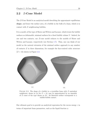
Our essential geometrical approximation is inspired by the early work of Ziman on
describing the Fermi-surface of copper [43]. The bubble volume V can be divided
into Z equivalent sections, each of which is to be represented approximately by a
circular cone (of volume Vc = V
Z
), as shown in Figure 2.3. The advantage of this
approximation is that it allows us to represent the bubble surface (referred to as
the cap) mathematically as a surface of revolution.
The bubble surface consists of a flat disk of area πδ2
(the contact area of neighbour-
ing bubbles) and an outer part which has a constant total curvature, terminating
at right angles to the cone surface. The flat disk and the outer part join smoothly;
there is no curvature discontinuity at the boundary.
As the liquid fraction φ is reduced, the contact area grows, and the separation of
bubble centres s is reduced according to:
s = 2(h + hc) = 2R0(1 − ξ) (2.1)
where h and hc are defined as the heights of the cap and cone, respectively (see
Figure 2.3). R0 is radius of a spherical sector of volume Vc and ξ is a dimensionless
deformation parameter (see Section 1.6). In the undeformed case, the radius R0
is identical to the equivalent sphere radius defined in Section 1.4.
Our aim is to compute the dimensionless excess energy ε, defined as
ε(ξ) =
A(ξ)
A0
− 1, (2.2)
where A(ξ) is the surface area of one of the cone caps, and A0 = 2πR2
0(1 − cos θ)
is the curved surface area of the undeformed cap, i.e. for ξ = 0.
For given ξ and solid angle Ω, we can calculate the surface area A of one of
these cones and its total volume Vc analytically, as outlined below and detailed in](https://image.slidesharecdn.com/0b1eb23b-c092-4b30-8aa1-2e454aa93edb-160425224409/85/Thesis_Robert_Murtagh_Corrected-41-320.jpg)
![Chapter 2. Z-Cone Model 28
Appendix A. Note that because each of the cones are identical the 4π steradian
solid angle of the bubble is divided equally between each contact such that
θ = arccos 1 −
2
Z
. (2.3)
The total surface area, per contact Z, of our bubble can be written as
A = Aδ + 2π
h
0
r(z) 1 +
dr(z)
dz
2
dz, (2.4)
where Aδ is the surface area of the contact and r(z) is the distance from a point
on curved surface to the central axis of the cone (see Figure 2.3). The second term
in equation (2.4) is the general expression for the surface area (of revolution) of
any curve given by r(z).
The volume under this curve is given by
V = π
h
0
r(z)2
dz +
πr(0)3
cot θ
3
. (2.5)
Utilising the Euler-Lagrange formalism [38] in a similar way to Lacasse et al. [27],
we can determine the minimum surface area A under the constraint of constant
volume (for details of the method see Appendix A).
To do this, we require boundary conditions on the curvature of the surface at two
points; where the curved surface meets the flat contact and where it meets the
cone.
dr(z)
dz z=h
= ∞ (2.6)
dr(z)
dz z=0
= cot θ. (2.7)](https://image.slidesharecdn.com/0b1eb23b-c092-4b30-8aa1-2e454aa93edb-160425224409/85/Thesis_Robert_Murtagh_Corrected-42-320.jpg)


![Chapter 2. Z-Cone Model 31
J(ρδ, Z) =
1
ρδ
x2
(x2
− ρ2
δ)f(x, ρδ, Z) dx, (2.12)
and
K(ρδ, Z) =
1
ρδ
x2
f(x, ρδ, Z) dx, (2.13)
with
f(x, ρδ, Z) =
Z2
4(Z − 1)
x2
(1 − ρ2
δ)2
− (x2
− ρ2
δ)2
−1
2
. (2.14)
Now we have all that we need to compare with numerical results which will be the
purpose of the rest of this chapter.
2.2.2 Dependence of Energy on Deformation and Liquid
Fraction
In this section, we focus on the comparison of the cone model with Surface Evolver
simulations of the face-centred cubic (fcc) structure which is observed experimen-
tally in wet foams [12]. Our model is directly applicable in this case since each
bubble has Z = 12 equivalent neighbours. In the dry limit, a bubble approaches
a rhombic dodecahedron. We will also show the results of Surface Evolver simula-
tions for a pentagonal dodecahedron, for which the cone model gives even better
agreement.
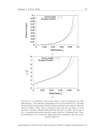
For the face-centred cubic structure (fcc) with Z = 12 the analytic solution is shown
in Figure 2.5(a), together with Surface Evolver calculations (see Appendix F for
details), which confirm its accuracy. This shows that for Z = 12 the dependence on
ξ is not quadratic, as stated by Lacasse et al. (from Surface Evolver calculations).
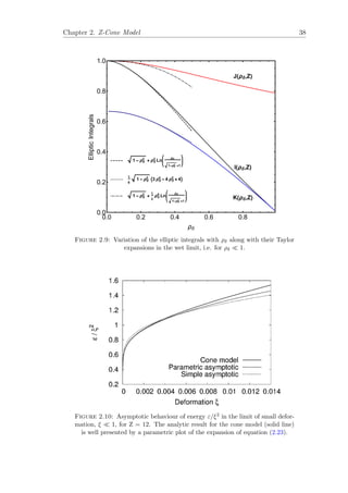
However, for smaller values of Z and over a limited range of ξ, a quadratic](https://image.slidesharecdn.com/0b1eb23b-c092-4b30-8aa1-2e454aa93edb-160425224409/85/Thesis_Robert_Murtagh_Corrected-45-320.jpg)

![Chapter 2. Z-Cone Model 34
Note that derivations of this equation and the key results from the cone model,
outlined in the rest of this chapter, are included in Appendix B.
For the cone model, we can show that
φc =
3 − 4
Z
Z − 1
. (2.16)
In the dry limit, φ → 0, our cone model data is well described by
ε(φ) = e0 − e1φ
1
2 (2.17)
which is the same form found for the Surface Evolver results, where it corresponds
to the decoration of film intersections with Plateau borders of finite cross-section
[2]. The values for the constants e0 and e1 are close to the true coefficients for the
given crystal structure, they vary as
e0 =
Z(Z − 1)
(Z − 2)2
1
3
− 1 (2.18)
and
e1 ∝
1
Z
(2.19)
respectively.
In the wet limit, φ → φc, the energy varies with the liquid fraction as
ε(φ) −
Z
18(1 − φc)2
(φc − φ)2
ln(φc − φ)
, (2.20)
see the discussion in Section 2.2.3.
Figure 2.8(a) shows that in the case of a regular pentagonal dodecahedron, the
cone model gives an even better prediction for ε(ξ) than for the fcc arrangement.](https://image.slidesharecdn.com/0b1eb23b-c092-4b30-8aa1-2e454aa93edb-160425224409/85/Thesis_Robert_Murtagh_Corrected-48-320.jpg)
![Chapter 2. Z-Cone Model 35
(a)
(b)
Figure 2.7: Voronoi cells for the (a) fcc and (b) pentagonal dodecahedral
crystal structures. The pentagonal faces of the pentagonal dodecahedron are
more similar in shape to the circular contacts of the Z-cone model than the
diamond-shaped faces of the fcc.
The reason for this is the symmetry of the faces, which can be seen in Figure
2.7, particularly for larger deformations. The basic assumption about the bubble
surfaces in the cone model is that they are rotationally symmetric; this means
that the contact areas themselves are always circular. Thus, we can expect a bet-
ter agreement between the cone model and the regular pentagonal dodecahedron
compared to the diamond-shaped faces of the fcc structure, despite both these
structures having the same number of contacts.
To further demonstrate the applicability of the cone model, in Figure 2.8(b) we
show the case of Z = 6; a bubble confined in a cube.
2.2.3 Asymptotic Form of the Energy-Deformation Rela-
tion
Now turning to the variation of energy with deformation, we note that the wet
limit is very subtle. As we saw in Sections 1.7.2 and 1.7.3, Morse and Witten [39]
and Lacasse et al. [27] have derived an asymptotic form for small deformation for
the dependence of excess energy ε on force F, proportional to F2
ln(F−1
).](https://image.slidesharecdn.com/0b1eb23b-c092-4b30-8aa1-2e454aa93edb-160425224409/85/Thesis_Robert_Murtagh_Corrected-49-320.jpg)
![Chapter 2. Z-Cone Model 36
(a)
(b)
Figure 2.8: Comparison of cone model predictions for ε(ξ) with Surface
Evolver simulations for Platonic solids. (a) Z = 12: a pentagonal dodeca-
hedron, and (b) Z = 6: a cube. We see good agreement, due to the underlying
symmetry of these shapes.
This was derived for the special cases of a droplet pressed against a flat surface
[39] and a drop compressed by two parallel plates (corresponding to Z = 2 in our
Z-Cone model) [27]. For present purposes it is more convenient to consider the
energy-deformation relation, which takes the corresponding asymptotic form](https://image.slidesharecdn.com/0b1eb23b-c092-4b30-8aa1-2e454aa93edb-160425224409/85/Thesis_Robert_Murtagh_Corrected-50-320.jpg)
![Chapter 2. Z-Cone Model 39
applying to any number of contacts Z near φc. However, the form of this interac-
tion differs for contacts gained away from φc; this is discussed in Chapter 5 where
we discuss the loss of the square faces in the Kelvin structure which occurs at
a liquid fraction significantly lower than the critical liquid fraction φc. Only for
larger values of ξ, and over a limited range, as a decreasing function of Z, may the
excess energy be reasonably well approximated by a quadratic, as will be discussed
in detail in Chapter 3.
The anomalous asymptotic (logarithmic) form adds a further complication to the
analysis of the approach to the wet limit in disordered foams, analogous to that
of the “jamming” problem in granular materials [8, 9]. If foam is to be taken as
a representative system for this problem, the validity of quadratic potentials in
granular packings must be questioned.
2.3 Conclusions and Outlook
In the limit of very small bubble-bubble contacts, Morse and Witten [39] and
Lacasse et al. [27] have suggested that the interaction between bubbles is log-
arithmic, rather than harmonic (see Sections 1.7.2 and 1.7.3). By treating the
bubble surfaces as deformable and geometrically approximating the volume, we
have introduced the Z-cone model which ties together a number of previous re-
sults [27, 39] with a single coherent picture. Importantly, our model moves away
from the Durian bubble model of overlapping spheres (see Figure 1.6 in Section
1.7.1), which is predominantly used in simulations of foam rheology.
We have presented a semi-analytical relation between the energy (i.e. surface area)
and the liquid fraction φ and correct asymptotic forms for the energy in the limits
of dry and wet foam, with prefactors dependent on Z. In particular, the variation
of energy with uniform, uniaxial deformation in the wet limit is consistent with
the anomalous behaviour first reported by Morse and Witten [39] and Lacasse et
al. [27], with a prefactor Z
2
.](https://image.slidesharecdn.com/0b1eb23b-c092-4b30-8aa1-2e454aa93edb-160425224409/85/Thesis_Robert_Murtagh_Corrected-53-320.jpg)
![Chapter 2. Z-Cone Model 40
In the form presented so far, the Z-cone model is strictly only applicable to a
limited number of cases, in which neighbours are equivalent, but it is possible to
pursue its generalisation to other ordered structures. This will be explored for the
Kelvin foam in Chapter 4. A further generalisation to bidisperse systems will be
the subject of Chapter 7.
The asymptotic variation of energy and forces in the wet limit is of some topi-
cal importance, because a wet foam is regarded as an ideal experimental system
with which to investigate jamming properties, since it has well-characterised con-
stituents without static friction [44]. However, theories of jamming often invoke
the kind of quadratic forces that we have now shown, with the Z-cone model, to
be qualitatively inappropriate for foams, in the wet limit. Is the presence of a log-
arithmic force and energy specific to bubbles, for which the surfaces are not rigid
but deformable and there is no static friction? While a definitive answer to this
question is beyond the scope of this work, a sharp transition between harmonic
and logarithmic forces for a finite rigidity of the particles seems unlikely. Thus,
the results presented here for bubbles call into question the validity of quadratic
potentials in granular packings.](https://image.slidesharecdn.com/0b1eb23b-c092-4b30-8aa1-2e454aa93edb-160425224409/85/Thesis_Robert_Murtagh_Corrected-54-320.jpg)
![Chapter 3
Applications of the Z-Cone Model
In Chapter 2, we introduced the Z-cone model of a bubble in the bulk of a foam
to understand the properties of foams in equilibrium. From this, we were able
to derive an approximate expression for the excess surface energy ε of a bubble
in terms of deformation and liquid fraction which demonstrated that there is a
logarithmic term which dominates the bubble-bubble interaction close to the wet
limit φc. This interaction was also shown to be inexpressible as a pair potential
since it depends explicitly on the number of neighbours of each of bubbles Z
which may, in principle, be different for each of the bubbles forming the contact.
By Taylor expanding the excess energy very close to the wet limit, we were able
to determine this critical form.
The aim of this chapter is to further our analysis of the implications of the Z-cone
model. While the presence of a logarithmic term at the wet limit rules out the
presence of a strictly harmonic interaction, the range of deformations where this
logarithmic correction is dominant is small. Away from this limit, the interaction
is approximately harmonic, as discussed by Lacasse et al. [27]. In Section 3.1 we
will show this for the Z-cone model.
We will also show how the Z-cone model can be used to determine the liquid
fraction profile and osmotic pressure of a foam.
41](https://image.slidesharecdn.com/0b1eb23b-c092-4b30-8aa1-2e454aa93edb-160425224409/85/Thesis_Robert_Murtagh_Corrected-55-320.jpg)
![Chapter 3. Applications of the Z-cone Model 42
3.1 Computation of the Effective Spring Con-
stant for the Bubble-Bubble Interaction
In this section, we will compute an effective Hookean spring constant, as a function
of contact number Z, for bubble-bubble interactions using the Z-cone model. As
we saw in Section 1.7.3, Lacasse et al. [27] proposed a power law form for the
excess energy ε as a function of the deformation ξ, given by equation (1.16), with
fitting parameters CZ and αZ.
The slightly odd form of the term in square brackets is due to the fact that this
expression is equivalent to ε = C (φc −φ)αZ
and has been converted to deformation
using the relation ξ = 1− 1−φc
1−φ
1/3
. Equation (1.16) was found to agree well with
Surface Evolver simulations of a bubble confined by a number of contacts Z in the
range ξ ∼ 0.02 − 0.1. In particular, αZ was found to rise from αZ = 2.1 for two
contacts to αZ = 2.5 for the fcc structure.
There are two key features of equation (1.16) which bear further investigation.
Firstly, the prefactor CZ depends on the number of contacts Z. This is consistent
with our findings from Chapter 2 in which we showed that the prefactor in the
logarithmic asymptotic form for the excess energy ε depends explicitly on the
number of contacts Z. Secondly, the power αZ is close to the harmonic value of
αZ = 2.
While a power law of the form of equation (1.16) is useful, it is not easy to visualise
the term in brackets as the displacement term in a Hookean spring model. As we
discussed in Section 1.6 when we defined the deformation ξ for the simple struc-
tures with Z equivalent neighbours that we are considering here, the deformation
can be simply related to the distance between bubble centres s which forms the ba-
sis of any spring model. For this reason, we choose to describe the bubble-bubble
interaction for higher values of the deformation as
ε ∝ ξα
. (3.1)](https://image.slidesharecdn.com/0b1eb23b-c092-4b30-8aa1-2e454aa93edb-160425224409/85/Thesis_Robert_Murtagh_Corrected-56-320.jpg)
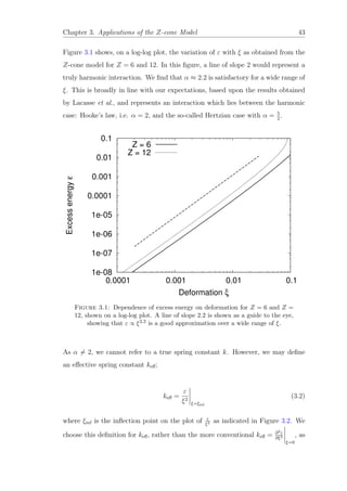
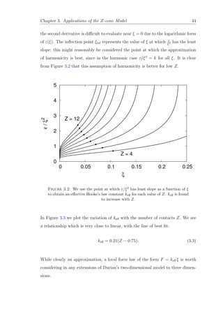
![Chapter 3. Applications of the Z-cone Model 45
0.4
0.6
0.8
1
1.2
1.4
1.6
1.8
2
2.2
2.4
2.6
4 5 6 7 8 9 10 11 12
keff
Z
Figure 3.3: The variation of the effective spring constant keff with the number
of contacts Z is well described by the linear relationship (3.3).
3.2 Osmotic Pressure in the Z-Cone Model
As we have seen, the Z-cone model provides us with analytic predictions for the
excess energy ε as functions of both deformation ξ and liquid fraction φ. Using
these analytic expressions, we will compute the osmotic pressure Π and from this
a liquid fraction profile for a foam at equilibrium under gravity. The osmotic
pressure, as it is defined in equation (1.3) is for any volume of foam V . In the Z-
cone model, however, we are considering an ordered foam with identical bubbles.
In this case, we can relate the reduced osmotic pressure to the excess energy ε of
a single bubble in the foam [12] by
˜Π(φ) = −3(1 − φ)2 ∂ε
∂φ
, (3.4)
where the derivative can be expressed as ∂ε
∂φ
= ∂ε
∂ξ
∂ξ
∂φ
(see equation (3.6)).](https://image.slidesharecdn.com/0b1eb23b-c092-4b30-8aa1-2e454aa93edb-160425224409/85/Thesis_Robert_Murtagh_Corrected-59-320.jpg)
![Chapter 3. Applications of the Z-cone Model 46
Figure 3.4 shows ˜Π(φ), as computed numerically for the Z-cone model using equa-
tion (2.9).
Figure 3.4: The variation of the reduced osmotic pressure ˜Π as a function of
liquid fraction φ, together with an empirical relationship proposed by H¨ohler et
al. to describe experimental data [12] for ordered foams. The data presented is
for Z = 12.
The dashed line in Figure 3.4 is an empirical relationship given by
Π(φ)
γ
R
= 7.3(φ − φc)2
φ−1
2 , (3.5)
which was obtained as a fit to experimental data for osmotic pressure measure-
ments carried out by H¨ohler et al. [12]. The Z-cone model gives a good ap-
proximation to this experimental relationship over the full range of liquid fraction
φ.
Although there is no explicit algebraic form for ˜Π(φ) from the Z-cone model,
over the entire range of liquid fraction φ, it is possible to provide an asymptotic](https://image.slidesharecdn.com/0b1eb23b-c092-4b30-8aa1-2e454aa93edb-160425224409/85/Thesis_Robert_Murtagh_Corrected-60-320.jpg)
![Chapter 3. Applications of the Z-cone Model 47
form in the wet limit. Taking equation (2.22) for the corresponding asymptotic
form of ε(ξ) along with the identity equation (2.15), and using the transformation
∂ε
∂φ
= ∂ε
∂ξ
∂ξ
∂φ
, results in
Π(φ)
γ
R
= −
Z
3
(1 − φ)2
(1 − φc)2
(φc − φ)
ln(φc − φ)
(3.6)
in the wet limit. This is also in good agreement with Surface Evolver data with
the appropriate choice of φc.
3.3 Liquid Fraction Profile
The liquid fraction profile for the Z-cone model was derived by considering the
reduced osmotic pressure ˜Π(φ) of the foam, which we defined in Section 1.5. We
saw that there is a simple relationship, equation (1.6), between the local liquid
fraction φ(˜x) at a reduced height ˜x above the bottom of the foam and the reduced
osmotic pressure ˜Π.
The reduced height which we have introduced is defined as ˜x = xR0
l2
0
with l0 the
capillary length. The capillary length l0 is a characteristic length scale used in
foams and is defined as the ratio of buoyancy forces to inertial forces [3] and has
been used by previous authors to define a single bubble layer in a wet foam as
l2
0
R0
[3]. Thus, the reduced height ˜x measures the height in the foam in terms of the
number of bubble layers, and so is useful in particular for experiments.
Expanding equation (1.6) into partial derivatives, we obtain a differential equation
for φ(˜x) which depends on ∂ ˜Π/∂φ:
∂φ
∂˜x
=
1 − φ(˜x)
∂ ˜Π
∂φ
, with φ(0) = φc. (3.7)](https://image.slidesharecdn.com/0b1eb23b-c092-4b30-8aa1-2e454aa93edb-160425224409/85/Thesis_Robert_Murtagh_Corrected-61-320.jpg)
![Chapter 3. Applications of the Z-cone Model 48
We can use equation (2.16) to obtain an expression for ε(φ) which we use with
equation (3.4) to solve this differential equation numerically, yielding a liquid frac-
tion profile for any Z. We choose Z = 12, as for fcc-ordered foams, and so equation
(2.16) gives a critical liquid fraction φc = 0.242. We plot the obtained liquid frac-
tion profile in Figure 3.5, and compare it to an empirical fit to experimentally
measured profiles for ordered foams [45]. Note that the experimental data has a
critical liquid fraction of 0.26.
While there is good agreement between the Z-cone model with Z = 12 and the
experimental data in the wet limit, there is a discrepancy at lower φ with the
wetness decaying more slowly that is predicted by the Z-cone model. One possible
source of this is the fact that Z = 12 does not hold throughout an ordered foam.
When φ < 0.07, bubbles tend to arrange in a Kelvin (bcc) structure more readily
than fcc [12]. We will discuss the bcc structure in detail in Chapters 4 and 5.
0
0.05
0.1
0.15
0.2
0.25
0 1 2 3 4 5
Liquidfractionφ
Reduced height x~
Z-cone model: Z = 12
Simple theory
Experimental data
Figure 3.5: The liquid fraction as a function of reduced height, obtained using
the Z-cone model with Z = 12, compared to a simple theoretical expression
from [2], and to an empirical expression for ordered monodisperse foams from
Maestro et al. [45]. The Z-cone model gives an adequate approximation of the
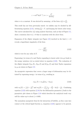
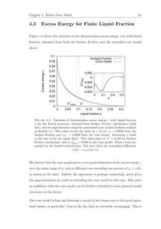
experimental data in the wet limit.](https://image.slidesharecdn.com/0b1eb23b-c092-4b30-8aa1-2e454aa93edb-160425224409/85/Thesis_Robert_Murtagh_Corrected-62-320.jpg)
![Chapter 3. Applications of the Z-cone Model 49
In the same figure we have also plotted an expression for φ(˜x) following from
Weaire et al. [2]:
φ(˜x) = ˜c ˜x +
˜c
φc
−2
. (3.8)
The derivation of this expression considers the vertical variation in cross-section
of a Plateau border, based on the hydrostatic pressure variation in the liquid;
together with a structural constant ˜c ≈ 0.333 related to the number of Plateau
borders per volume in a Kelvin foam [2]. The resulting equation (equation (3.8)),
presented in this form for the first time, is a surprisingly good description of the
experimental data, and has an appealingly simple form.
3.4 Conclusions and Outlook
In Chapter 2, we used the Z-cone model to identify a logarithmic form for the
excess energy ε, close to the wet limit. This showed that the interaction between
bubbles in this limit is clearly not harmonic, which is a commonly used model of the
interaction in computer simulations, in particular the Durian model (see Section
1.7.1). However, approximate harmonicity could be inferred for the interaction
slightly further away from φc. We examined the validity of such an assumption,
showing that while it may represent a reasonable approximation for low Z, it is
far from acceptable for Z higher than about 7. This significantly reduces the
validity of such an assumption for simulations of three-dimensional foams, where
the average number of contacts per bubble is typically between 12 and 14 [3]. We
proposed that a more appropriate form for high numbers of contacts would be to
consider a power law with an exponent of 2.2.
We have further analysed the Z-cone model from Chapter 2, using it to compute
the reduced osmotic pressure Π(φ) as a function of liquid fraction. We have shown
that the results from the Z-cone model agree well with experimental findings [12].
Expanding on the theme of asymptotic forms for the wet limit from Chapter 2,](https://image.slidesharecdn.com/0b1eb23b-c092-4b30-8aa1-2e454aa93edb-160425224409/85/Thesis_Robert_Murtagh_Corrected-63-320.jpg)
![Chapter 3. Applications of the Z-cone Model 50
we have derived an analytical expression for the reduced osmotic pressure ˜Π close
to φc which agrees well with the results of Surface Evolver for the case of Z = 12.
This provides further confidence in the power of our model to describe foams in
equilibrium, despite the approximations used in its conception.
Furthermore, we have used the osmotic pressure to compute a liquid fraction profile
for a foam which provides an adequate approximation to experimental data for
the fcc structure in the wet limit. Some deviation is observed for intermediate
liquid fractions which can most likely be attributed to the fact that as the liquid
fraction decreases in experiment, the fcc structure ceases to be the lowest energy
crystal structure with the bcc structure being strongly preferred below about φ =
0.07 [12]. Due to the Z-cone model underestimating the excess energy of the
fcc structure compared to the Surface Evolver (see Figure 2.6), this crossover is
observed closer to φ = 0.1 (see Chapters 4 and 5).](https://image.slidesharecdn.com/0b1eb23b-c092-4b30-8aa1-2e454aa93edb-160425224409/85/Thesis_Robert_Murtagh_Corrected-64-320.jpg)
![Chapter 4
Application of the Cone Model to
a Kelvin Foam
In the physics of foams, the structure envisaged by Kelvin [46] has played a cen-
tral role as a prototype, even though it is now known not to be the structure of
lowest energy for a monodisperse dry foam [47]. The Kelvin structure is based on
the bcc lattice, shown in Figure 4.1, which has eight nearest neighbours and six
next nearest neighbours. Various authors have already applied Surface Evolver
simulations to the dry Kelvin structure [12]. In particular, H¨ohler et al. have used
it when discussing foam structure in the case of finite liquid fraction [12].
In this chapter, we will show that the Z-cone model, introduced in Chapter 2
to model bubbles in contact with Z equivalent neighbours, can be extended to a
more general cone model which incorporates unequal contacts. Although various
approximations are involved in the new formulation, the model retains the char-
acter of the original Z-cone model as there are no adjustable parameters. This
represents the first step in extending this geometric idea to more general ordered
foam structures and, as we shall see, the generalised method that we describe here
can easily be adapted for other ordered structures.
As was the case for the Z-cone model, our primary goal is to present an approx-
imation of the excess energy ε of the Kelvin cell. The results of this model will
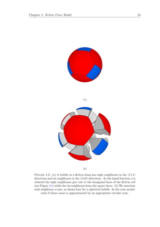
51](https://image.slidesharecdn.com/0b1eb23b-c092-4b30-8aa1-2e454aa93edb-160425224409/85/Thesis_Robert_Murtagh_Corrected-65-320.jpg)


![Chapter 4. Kelvin Cone Model 60
4.2 Excess Energy of the Dry Kelvin Cell
When considering the energy of the Kelvin structure, it is worth recalling what
Kelvin himself was able to do at the outset [46]. He was concerned only with the
dry foam limit of φ = 0, for which he produced a remarkably accurate description
of the bubble shape which came to bear his name, shown in Figure 4.1(b). He
recognised the importance of crystal symmetry which implies that the quadrilateral
faces are flat, while the hexagonal ones are not, and applied Plateau’s rules for
the angles of intersection of faces, together with the requirement that the total
curvature of the hexagonal faces is everywhere zero. His numerical calculation by
hand of the approximate form of the hexagonal faces was a veritable tour de force.
But Kelvin did not proceed to estimate the surface area of his new structure, even
though this bore directly on the motivation for the work. It appears that this was
first evaluated one hundred years later, when Princen and Levinson [20] computed
the surface area numerically by using a discretisation into flat segments.
The result was expressed in terms of the relative surface area A
A0
, where A0 is
the surface area of a sphere with the same volume of the polyhedron. Note that
the relative surface area is nothing more than ε + 1, according to our definition
of excess energy ε from Section 1.6. The computed value of A
A0
for the Kelvin
cell is 1.0970, a decrease from the value of 1.0990 for the planar-faced truncated
octahedron, which to Princen and Levinson appeared “surprisingly small” [20].
However, it is possible to offer an alternative estimate of the dry Kelvin excess en-
ergy by adjusting the angles of the truncated octahedron to conform with Plateau’s
rules (see Section 1.2) and which may have applications to other such structures.
In this way, we obtain a value of A
A0
= 1.0968. As this is not central to our dis-
cussion in this chapter, we leave a discussion of the details of this estimate to
Appendix E. We were also able to obtain a value of εK0 = 0.0970 from Surface
Evolver calculations which agree with the value of Princen and Levinson.
We will shift our focus in the following section to using a comparison of the ex-
tended cone model outlined above with Surface Evolver simulations.](https://image.slidesharecdn.com/0b1eb23b-c092-4b30-8aa1-2e454aa93edb-160425224409/85/Thesis_Robert_Murtagh_Corrected-74-320.jpg)
![Chapter 4. Kelvin Cone Model 62
in contrast to the simple Z-cone model where the comparison with Surface Evolver
is noticeably worse as the dry limit is approached, i.e. for large deformations (see
Chapter 2). The reason that the cone model so closely agrees with Surface Evolver
for the Kelvin structure is primarily related to the shape and relative size of the
faces in the the Kelvin cell.
In Section 2.2.2, we noted that for Z = 12 the cone model agreed better with
the pentagonal dodecahedral structure than the fcc structure due to the high
symmetry of pentagonal faces (i.e. the pentagons better resembled the circular
contacts assumed by the cone model than the diamond-shaped faces of the fcc cell).
The degree of symmetry increases with the number of sides and so the presence
of eight large hexagonal faces should significantly improve the accuracy of our
approximate model. As the six square faces only account for about one quarter of
the total surface area of the dry Kelvin cell, the effect of the less symmetric square
faces is not as important.
The value of φ at which the six 1 0 0 contacts vanish is given by φ∗
= 0.108 for
the exact case and φ∗
cone = 0.092 for the cone model, indicated by the dashed lines
in Figure 4.4. It is worth noting that Weaire et al. [48] arrived at a remarkably
accurate early estimate of φ∗
≈ 0.11 by a crude argument based on ratios of
Plateau border widths. A clear difference exists however for the value of φ∗
from
these two methods. The contact loss in the cone model precedes that in the Surface
Evolver computations (i.e. at a lower liquid fraction). This discrepancy between
the values of φ∗
obtained is a direct result of the approximations of the cone model.
Although our cone model agrees well with Kelvin cell due the symmetric shape of
the hexagonal faces, the approximation of circular faces which we must make is not
sufficiently precise here and this gives rise to the observed discrepancy. The small
difference in ν, the equivalent ratio of the height of two cones, for the cone model
from the value of
√
3
2
and the approximation of circular cones are also important
contributing factors. This interpretation is supported by the fact that the critical
liquid fraction φc for the wet limit predicted from the cone model is φc, cone = 0.319
which is a very good approximation to the value of φc = 0.320 for the Kelvin foam
[2].](https://image.slidesharecdn.com/0b1eb23b-c092-4b30-8aa1-2e454aa93edb-160425224409/85/Thesis_Robert_Murtagh_Corrected-76-320.jpg)

![Chapter 5
Contact Losses in the Kelvin
Foam
We saw in Chapter 4 that the Kelvin structure, consisting of a body-centred cubic
(bcc) arrangement of bubbles (see Figure 4.1), provides a prototypical structure to
extend the cone model for unequal contacts. The significance of the Kelvin foam
as a prototype and our interest in it extends further, however. It also represents a
well-defined structure that can be used for the study of a general feature of foams,
namely the gain or loss of a face at some critical liquid fraction φ∗
.
The Kelvin structure is stable with respect to small deformations for liquid volume
fractions φ up to about φ ≈ 0.11 [13]. For φ > 0.11 the Kelvin foam becomes un-
stable, and the close-packed fcc and hcp structures become energetically favourable
[12]; the lattices for these structures are given in Section 1.4.
In experiments it is found that the fcc structure gives way to the bcc structure
gradually as the liquid fraction is decreased with regions of both fcc and bcc
present in the foam [12]. However, this structural transition from fcc to bcc would
be sharp with the cone model, occurring precisely at a single value of the liquid
fraction. The reason for this sharp transition is that the cone model treats a foam
as a collection of identical bubbles with a precisely specified crystal geometry
which is difficult to replicate in experiments.
65](https://image.slidesharecdn.com/0b1eb23b-c092-4b30-8aa1-2e454aa93edb-160425224409/85/Thesis_Robert_Murtagh_Corrected-79-320.jpg)
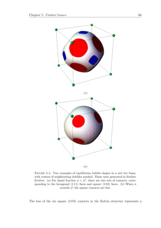
![Chapter 5. Contact Losses 67
structural transition tied to the variation of liquid fraction. An illustration of the
loss of the square faces is shown in Figure 5.1. As φ is increased from 0 to its
maximum value of φc = 1 −
√
3π
8
, at which the bubbles are spheres (see Section
1.3), the areas of the square contacts are observed to shrink with increasing φ prior
to disappearing at a liquid fraction φ∗
< φc.
In examining the contact losses in the Kelvin structure, we will focus particularly
on the details of the variation of excess energy ε with liquid fraction φ close to
the liquid fraction at which contact is lost with the six neighbours in the 1 0 0
crystal directions. By using this generalised cone model, in addition to Surface
Evolver computations (see Appendix F for further details of the Surface Evolver
calculations), we will arrive at an empirical expression for the variation of energy
close to this point. While it also features a logarithmic term, the functional form
is distinctly different to that found for the Z-cone model (see equation (2.20)).
5.1 Shrinking of the Square Faces
In Section 4.3, we discussed the variation of the excess energy ε with liquid fraction
for the Kelvin cell and noted that the square 1 0 0 contacts were lost at a liquid
fraction φ∗
. The precise value of φ∗
= 0.108 is slightly higher for the Surface
Evolver (which represents the exact Kelvin cell with curved faces) than the value
of φ∗
cone for the cone model due to the approximation inherent in the cone model
(see Section 4.3 for further details).
This shrinking of the contact areas to zero is particularly sudden (i.e. occurs over a
very short range of liquid fraction) close to φ∗
which raises the question of whether
the Kelvin structure becomes unstable due to the loss of the square contacts at φ∗
or whether the instability occurs prior to the loss of these contacts. Indeed, the
association of this contact loss with instability is not new, dating back to some
incidental remarks of Weaire et al. [48] who were inspired by the instability of bcc
metals.](https://image.slidesharecdn.com/0b1eb23b-c092-4b30-8aa1-2e454aa93edb-160425224409/85/Thesis_Robert_Murtagh_Corrected-81-320.jpg)


![Chapter 5. Contact Losses 70
Figure 5.3: The derivative of the excess energy with respect to liquid fraction,
dε
dφ over the full range of liquid fraction obtained from the cone model. The
vertical dashed lines mark the critical values of liquid fraction for which contacts
are formed/lost in this structure. There is a clear discontinuity of slope at
φ = φ∗
cone = 0.092, i.e the point at which the square faces corresponding to
next-nearest neighbour contacts are formed/lost.
For dε
dφ
at φ = φ∗
, we did not find an analytical expression from our new cone
model. This is due to the additional geometrical complications which are inherent
in this model, as we discussed in Chapter 4. However, the following empirical
expression is a reasonably good description of the data which we show in Figure
5.4(b),
dε
dφ
= b1 +
b2
(ln(φc − φ))2 (5.2)
There is a clear discontinuity of the slope of dε
dφ
at φ = φ∗
cone which is clearly visible
in Figure 5.4(b).
Of note is the presence of logarithmic terms in both expressions, a feature known
from studies of the bubble-bubble interactions [27, 39] (see Section 1.7). The
discrepancy between the forms of equations (5.1) and (5.2) suggests that results](https://image.slidesharecdn.com/0b1eb23b-c092-4b30-8aa1-2e454aa93edb-160425224409/85/Thesis_Robert_Murtagh_Corrected-84-320.jpg)

![Chapter 5. Contact Losses 72
It has been argued that the limit of mechanical stability of the Kelvin structure
was due to the loss of the square faces [49]. A bcc crystal of interacting points
is well known to require second-nearest-neighbour interactions to stabilise when
simple pairwise potentials are applied. This appeared indeed supported by Phelan
et al. [23] who found a negative elastic constant at values of of φ > 0.11, i.e. close
to the value of φ = 0.11±0.005 that these authors identified for the face loss. New
preliminary Surface Evolver calculations suggest that the elastic constant changes
sign for φ near φ∗
but this work is in its nascent stages and will be investigated
further in future work.
At present, the calculation of such elastic constants with the cone model is limited
to the reduced uniaxial modulus µ(φ) for simple cases of Z = 2 and Z = 6 due to
their particularly simple symmetries. While the results of these early calculations
are in agreement with the results of previous work by both Buzza and Cates [50]
and Lacasse et al. [27], showing a characteristically logarithmic onset of µ(φ) at
the point of contact formation, it is not yet clear how to extend this approach to
the Kelvin cell. Nonetheless, the sharp contrast in behaviour seen in Figure 5.4 for
the excess energies of the different faces, suggests that further analysis of the loss
of the square 1 0 0 could show an instability at a liquid fraction slightly lower
than φ∗
cone.
5.3 Conclusions and Outlook
We have made use of the extended the cone model of Chapter 4 to investigate the
variation of the excess energy ε with liquid fraction φ close to the loss of both the
square and hexagonal contacts of the Kelvin cell.
We see two distinct contact losses; the loss of the hexagonal 1 1 1 faces at the wet
limit, φc, and of the square 1 0 0 faces away from the wet limit at φ∗
, resulting
in two distinctly different variations of energy with liquid fraction. Both feature
logarithmic terms in the respective derivative of energy with respect to liquid](https://image.slidesharecdn.com/0b1eb23b-c092-4b30-8aa1-2e454aa93edb-160425224409/85/Thesis_Robert_Murtagh_Corrected-86-320.jpg)

![Chapter 6
Evolution of a bubble on a liquid
surface containing one or two gas
species
In this chapter, we will be looking at the shape of a bubble at a liquid surface using
the mathematics of minimal surfaces of revolution, an approach which was also at
the heart of the cone model which has been introduced previously. Once again,
we shall focus on the theoretical and computational aspects of the problem before
utilising these to understand the results of experimental studies. In particular, we
aim to model the temporal evolution of a single bubble at a liquid surface, taking
account of its detailed shape, for two-component gas mixtures.
Bubbles containing more than one type of gas are increasingly being used in mod-
ern experimental foam physics. It has been shown both computationally [51] and
experimentally that the addition of a low solubility gas significantly extends the
lifetime of the foam [52] by resisting Ostwald ripening or “coarsening” [3]. The ad-
dition of perfluorohexane gas (PFH) to bubbles of air or nitrogen is now a standard
procedure in foam drainage and rheology experiments [53] that run over several
hours.
74](https://image.slidesharecdn.com/0b1eb23b-c092-4b30-8aa1-2e454aa93edb-160425224409/85/Thesis_Robert_Murtagh_Corrected-88-320.jpg)
![Chapter 6. Bubble Evolution 75
Despite the growing experimental interest in mixed gas systems for the purpose
of inhibiting coarsening (over several days, as in the experiments of Meagher et
al. [17]), there are a number of observations of growing mixed gas bubbles [54],
particularly at foam/air interfaces, which have yet to be fully explained [55]. The
origin of this behaviour is connected to the addition of relatively insoluble gases,
such as PFH, to air in the bubbles [56], as we will show in this chapter.
6.1 Introduction to Surface Bubbles
The shape of a single bubble at a liquid surface consists of two parts which meet in
a circular ring of contact with a radius of xc (see Figure 6.1). In what follows, we
will regard the radius xc as a measure of the bubble size since it is easily measured
in experiments. Above the ring of contact, the bubble surface is a spherical cap
in contact with the atmosphere while below this ring, the bubble is in contact
with the liquid and forms a sessile droplet [57]. The examples shown in Figure
6.1 were computed numerically using a method developed by Princen [57] (for
details see Appendix G), for the case of an infinitesimally thin liquid film. In
reality, this liquid film has a finite thickness which is a function of both position
and time. We chose a numerical approach here due to the difficulty of obtaining
analytical solutions for this shape on a liquid surface. For the similar shape of
a hemispherical bubble sitting atop a flat substrate with liquid Plateau borders,
however, Teixeira et al. [58] adduced an approximate analytical solution for the
shape of the Plateau borders in the limit of small Plateau border sizes.
In contrast to our discussion of the cone model, the actual bubble size xc is crucial
to our discussions in this chapter. The primary reason for this is that a bubble
at the surface of a liquid is subject to the opposing forces of surface tension,
which tries to draw liquid out of the bulk (effectively pushing the bubble down),
and inertial forces (gravity) which cause the bubble to effectively rise out of the
liquid; the interplay between these two forces determines the position of the ring
of contact [2] and so the overall shape of the bubble.](https://image.slidesharecdn.com/0b1eb23b-c092-4b30-8aa1-2e454aa93edb-160425224409/85/Thesis_Robert_Murtagh_Corrected-89-320.jpg)
![Chapter 6. Bubble Evolution 76
The balancing of these two forces defines a length scale, known as the capillary
length l0 (see Chapter 1), which demarcates the bubble size regimes for which
gravity or surface tension is the dominant force. Accordingly, the capillary length
l0 is represented by the formula
l0 =
σ
∆ρg
(6.1)
where σ represents surface tension, ∆ρ the difference in density between the liquid
and gas phases and g is the acceleration due to gravity. Bubbles which are much
smaller than the capillary length become gradually submerged below the liquid
surface, as shown in Figure 6.1, while bubbles much larger than the capillary length
are almost hemispherical. The capillary length for the commercially available
detergent Fairy Liquid, which we use in the experiments detailed in Section 6.5
below, is l0 ≈ 1.693mm [2, 59], which is fairly typical for the surfactants used in
foam experiments.
Thus far we have discussed how the shape of a bubble at a liquid surface depends
upon the size of the bubble. However, we have yet to comment on the mechanism
by which a surface bubble evolves in time, i.e. by diffusion, or the role played by
the gas composition. We pick up both of these threads in the next section which
will be an introduction to diffusion in bubbles.
6.2 Diffusion in Gas Mixtures
In Chapter 1 (see Section 1.1), we noted that coarsening is the name given to
the process of gas diffusion between neighbouring bubbles in a foam [2]; a gen-
eral consequence of which is that relatively large bubbles get larger and relatively
small bubbles get smaller over time. The treatment of this subject in the foams
community often focusses on average bubble quantities for bulk foams. For exam-
ple, it is found that the average bubble radius grows with time with a power law
exponent dependent on the liquid fraction φ of the foam [60]. For dry foams, the](https://image.slidesharecdn.com/0b1eb23b-c092-4b30-8aa1-2e454aa93edb-160425224409/85/Thesis_Robert_Murtagh_Corrected-90-320.jpg)
![Chapter 6. Bubble Evolution 77
(a) xc
l0
= 11 (b) xc
l0
= 2.3
(c) xc
l0
= 11
(d) xc
l0
= 2.3
Figure 6.1: Exemplary calculations of the shape of a bubble on a liquid surface.
(a) Bubbles much larger than the capillary length l0 are roughly hemispherical
while (b) bubbles whose size xc is close to or below the capillary length take
on more complicated shapes as they are partially submerged beneath the liquid
surface. The extent of the spherical cap is shown in red while the liquid surface
is shown in green. 2D cross-sections of the bubbles shown in (a) and (b) are
shown in (c) and (d). (xc, zc) marks the ring of contact (see above) separating
the spherical cap in contact with the atmosphere from the rest of the bubble.
This is also the point where the liquid tail (marked in green) meets the spherical
cap of width 2xc. L indicates the height of the liquid surface above the bottom
of the bubble far from the edge of the bubble (i.e when the surface becomes
flat).
average bubble radius is found to grow as t1/2
while for wet foams, the exponent
law changes to 1/3 [61]. The introduction of insoluble gases is known to inhibit
coarsening and so we focus on the diffusion characteristics of a single bubble to
better understand the effect of using mixtures of gases.
Under the influence of a concentration or pressure gradient, a soap film acts as
a permeable membrane, with a permeability coefficient k, allowing gas to diffuse
across it. The gas pressure pg in a bubble is higher than the atmospheric pressure
P0 (see Section 1.2) by an amount ∆p = pg − P0 = 4σ
Rc
where Rc is the radius of](https://image.slidesharecdn.com/0b1eb23b-c092-4b30-8aa1-2e454aa93edb-160425224409/85/Thesis_Robert_Murtagh_Corrected-91-320.jpg)
![Chapter 6. Bubble Evolution 78
curvature of the thin liquid film. This creates a pressure gradient across the surface
of the bubble. Considering the soap film as a pair of surfactant layers separated by
bulk liquid, it has been both proposed theoretically and observed experimentally
that the permeability coefficient of the film is inversely proportional to its thickness
for thick films [59, 62]. One such theoretical expression, forwarded by Princen and
Mason, illustrates this point:
k =
DH
hf + D
kml
, (6.2)
where hf is the film thickness, D is the diffusion coefficient of the gas, kml is
the monolayer permeability and H is gas solubility. For very thin films, the per-
meability is controlled by the permeability of the surfactant monolayers. The
permeability coefficient depends linearly on the solubility of the gas and the diffu-
sion coefficient of the film. Also of note is that the dependence of k on the diffusion
coefficient drop out if D/kml hf .
Diffusion through the film into the atmosphere is not the only possible diffusion
mechanism for a bubble floating at a liquid surface. Gas can be exchanged with
the liquid at a rate which depends upon the gas saturation level in the liquid
[63]. For example, an oversaturation of gas in the liquid manifests itself as an
effective overpressure in the liquid, creating a gas pressure difference between the
bubble and the surrounding liquid which tends to drive gas from the liquid into
the bubble. This is also known as outgassing [2, 3]. It is also possible for some
gas to diffuse into the bubble from the atmosphere due to local differences in the
gas concentration.
Given all of the potential processes associated with even the simplest case of a
single bubble floating at a liquid surface, we are forced to make a number of
simplifications to arrive at a tractable model for bubble evolution. We shall treat
the permeability coefficient as a constant for each of the gases in our bubble (thus
also fixing the solubilities). To do this, uniform and constant thickness in the thin
film of the bubble is assumed, as is the case with experiments in which the bubble](https://image.slidesharecdn.com/0b1eb23b-c092-4b30-8aa1-2e454aa93edb-160425224409/85/Thesis_Robert_Murtagh_Corrected-92-320.jpg)
![Chapter 6. Bubble Evolution 79
is left to drain for twenty-four hours before measuring its permeability [3, 59]. In
consideration of the bubble shape, the film is taken to be infinitesimally thin so
that the radius of the ring of contact xc can be well-defined. It then must also
be assumed that the liquid is sufficiently saturated with the gases under constant
temperature, to ensure that there is no net exchange of gases between the bubble
and the liquid.
In making these assumptions, we can begin to build a theoretical understanding
of the importance the diffusion of different gases has on the evolution of a bubble
on a liquid surface. In particular, how the bubble in question develops depending
on certain factors (size, capillary length, etc.) in two distinct cases:
1. Case One: We consider a bubble which contains a single, soluble gas that
is identical to the gas in the surrounding atmosphere, albeit at a different
pressure. We treat the corresponding permeability coefficient as constant in
time and denote it as kB.
2. Case Two: We consider a bubble which contains a mixture of two gases;
one of which has the same properties as in Case One above. The second gas
present is a low solubility or non-diffusive gas, which is not present in the
surrounding atmosphere and has a permeability coefficient denoted by the
symbol kA. We will consider two instances in this case: one in which kA = 0
which corresponds to a perfectly non-diffusing or insoluble gas and also the
more realistic case of a low solubility gas where kA kB.
This process of gas diffusion can be effectively modelled via Fick’s First Law [59]
which for a single gas, as in Case One, gives the change in the bubble volume ∆V
in time ∆t as
− ∆V =
kBAc∆p
P0
∆t, (6.3)
where Ac is the surface area of permeation, ∆p the pressure difference across the
surface of the bubble and kB is the permeability coefficient of the gas. As the total
pressure difference ∆p is always positive, the bubble volume shrinks over time](https://image.slidesharecdn.com/0b1eb23b-c092-4b30-8aa1-2e454aa93edb-160425224409/85/Thesis_Robert_Murtagh_Corrected-93-320.jpg)
![Chapter 6. Bubble Evolution 80
with a power law of t
1
2 [64, 65], as was observed previously by others, in particular
Princen and Mason [59]. We will return to the discussion of this in later sections.
In the case of mixtures of gases, the situation is more complicated. Dalton’s Law
of partial pressure states that the total pressure in a mixture of (ideal) gases is
equal to the sum of the partial pressures of each of the individual gases in the
mixture [51]. For a mixture of ideal gases, as in Case Two (here denoted A and
B), of differing permeabilities kA and kB we must consider not the total pressure
difference in Fick’s Law, but the partial pressure differences for each component of
the mixture. The partial pressure of a gas in a mixture is the pressure that the gas
would have if it occupied the volume of the entire mixture [51]. Mathematically,
it is defined as
pi =
Vi
Vtot
ptot = xiptot (6.4)
where Vi is the volume of one of the component gases, Vtot is the total volume of the
mixture (i.e. the bubble volume). The volume fraction xi can also be thought of
as the mole fraction of each gas component for gases which are similar in molecular
size. With this definition for the partial pressure, the appropriate version of Fick’s
Law of Diffusion for a mixture of gases [59] is given by the formula
−∆V =
2
i
kiAc
P0
∆pi∆t
= Ac∆t kA
(pA − pA)
P0
+ kB
(pB − pB)
P0
(6.5)
where the barred quantities denote properties of the atmosphere (see Figure 6.1).
Comparing this expression to equation (6.3), we see that the introduction of partial
pressures allows for a richer bubble evolution process than is the case for a single
gas. In addition to the shrinking evident in single gas bubbles, a mixed gas bubble](https://image.slidesharecdn.com/0b1eb23b-c092-4b30-8aa1-2e454aa93edb-160425224409/85/Thesis_Robert_Murtagh_Corrected-94-320.jpg)
![Chapter 6. Bubble Evolution 81
may grow in time depending on the permeabilities kA, kB of the two gases and
the partial pressure differences of the two gases.
The criterion which demarcates the boundary between growing and shrinking be-
haviour for these bubbles is obtained by considering ∆V = 0 in equation (6.5).
Furthermore, for the simplest case of a single bubble open to the atmosphere,
we have derived a simple analytic expression (see Appendix H) for this boundary
between growing and shrinking behaviour given by
kA
kB
= 1 +
1
x∗
A
P0
P0 + 4σ
Rc
− 1 . (6.6)
Equation (6.6) expresses the fact that for any mixture of gases with a fixed ratio
of permeabilities kA
kB
and for any bubble size Rc, there is a critical concentration
x∗
A of gas A for which the bubble neither grows nor shrinks. This is illustrated
for different bubble sizes in Figure 6.2. If the permeability of gases A and B is
similar (such as nitrogen and oxygen in air) and the concentration of A is low, then
the bubble is likely to shrink. However, for mixtures of PFH and air, a common
mixture for inhibiting coarsening, where the permeabilities differ by orders of
magnitude [66], the bubble will grow in time.
It is important to mention here that equation (6.6) (and hence Figure 6.2) is
derived for a surrounding atmosphere which is “very large” and initially contains
only gas B (see Appendix H for the full derivation). By very large, we mean that
the volume of gas A which diffuses from the bubble into the atmosphere does
not noticeably change the concentration of this gas A in the atmosphere. In
an experiment, this will only ever be an approximation and so Figure 6.2 serves
primarily as a very good qualitative description for the behaviour of a bubble of
a given size (see equation (H.4) for the general form of equation (6.6) applicable
to experimental systems).](https://image.slidesharecdn.com/0b1eb23b-c092-4b30-8aa1-2e454aa93edb-160425224409/85/Thesis_Robert_Murtagh_Corrected-95-320.jpg)
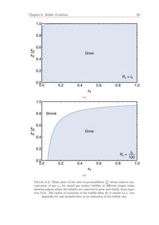
![Chapter 6. Bubble Evolution 83
Finally, we should note that we can equally well consider the critical concentration
x∗
B of the second gas B in the mixture since volume conservation requires that
xA + xB = 1. (6.7)
6.3 Simulations of the Evolution of a Single Bub-
ble
Examining both cases described above, we will describe simulations of growing and
shrinking bubbles at a liquid surface, taking into account the precise shape of the
bubble. As seen in Figure 6.1, xc is a suitable proxy for the bubble size since it is
most readily measured in an experiment by photographing from above. The results
of our simulation are expressed in the dimensionless quantities xc
l0
and t
l0
kB
for
bubble size as a function of time. For the computation of this volume-dependent
shape, an algorithm is used that was originally proposed by Princen [64]. This
algorithm enables the calculation of the precise shape of the bubble as a function
of time, achieved by numerical integration of a set of three coupled, ordinary
differential equations describing the boundary of the bubble (see Appendix G for
further details of the algorithm).
6.3.1 Case One: Simulation Results for the Shrinking Bub-
ble
In Case One, we examine a bubble of size xc that is initially much larger than the
capillary length and contains a single, soluble gas of permeability kB, for example
nitrogen (N2).
The volume change at each time step is calculated as a function of time from the
discrete form of Fick’s First Law, equation (6.3), which we introduced in Section](https://image.slidesharecdn.com/0b1eb23b-c092-4b30-8aa1-2e454aa93edb-160425224409/85/Thesis_Robert_Murtagh_Corrected-97-320.jpg)
![Chapter 6. Bubble Evolution 84
6.2. The contact area of permeation Ac and the pressure difference ∆p are updated
at each timestep.
In this case, the pressure difference is simply
∆p =
4σ
Rc
. (6.8)
Figure 6.3 shows the shrinkage of the bubble size xc as a function of time. The
guiding line, shown in dashed red, indicates a power law scaling behaviour of the
bubble size xc of
x2
c(t) − x2
c(0) ∝ −(t − t0) (6.9)
for bubbles much larger than the capillary length, as has been previously observed
experimentally [65]. The near hemispherical shape of large bubbles (Figure 6.1) is
at the heart of such scaling as will be demonstrated in Section 6.4.1.
It is notable that, as it comes close to the capillary length, the scaling of xc(t)
breaks down due to the decrease in bubble size xc which is accompanied by a
significant deviation of the shape from a hemisphere.
Given that a bubble with a single soluble gas shrinks, it is natural to wonder where
this case fits into the overall picture of growing and shrinking bubbles represented
by the phase plots of Figure 6.2.
In simplest terms, the case of a single soluble gas bubble is equivalent to a mixture
for which kA
kB
= 1. Thought of in this way, it is clear that the concentration xA
is equal to zero and we can identify the single gas bubble as occupying a point
at the top left corner in the phase plots of Figure 6.2. Despite the fact that the
region denoting shrinking behaviour is significantly reduced for larger and larger
bubbles, the top left corner will always be contained in this region and so we see
that such bubbles will always shrink, irrespective of the bubble size.](https://image.slidesharecdn.com/0b1eb23b-c092-4b30-8aa1-2e454aa93edb-160425224409/85/Thesis_Robert_Murtagh_Corrected-98-320.jpg)
![Chapter 6. Bubble Evolution 85
Figure 6.3: Computation of the time dependence of bubble size xc for a single
gas bubble, with a permeability coefficient kB, on a liquid surface. The dot-
dashed line shows the simulation data for xc(t). The red dashed line is a guide to
the eye indicating the slope of the scaling x2
c(t) − x2
c(0) ∝ −(t − t0), consistent
with previous studies [65]. The inset shows the strong deviations from this
scaling law for xc 7l0.
6.3.2 Case Two: Simulation Results for the Growing Bub-
ble
We move now to examining Case Two in which the single gas of permeability kB
(soluble) is mixed with a second gas with a different permeability kA (insoluble).
The volume change at each time step is calculated in this case from Fick’s Law
for mixtures, equation (6.5), and again, as for Case One, the contact area of
permeation Ac and the partial pressure differences ∆pA = pA − pA and ∆pB =
pB − pB are updated at each time step.](https://image.slidesharecdn.com/0b1eb23b-c092-4b30-8aa1-2e454aa93edb-160425224409/85/Thesis_Robert_Murtagh_Corrected-99-320.jpg)

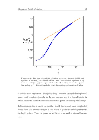
![Chapter 6. Bubble Evolution 88
6.3.2.2 The Effect of Permeability: kA kB
We showed in the previous section that the hemispherical shape of surface bubbles
much larger than the capillary length l0 gives rise to a clear power law scaling
behaviour with time. However, the choice of our initial conditions, in particular
the choice of kA = 0, represent a special case.
In real experimental systems (see Section 6.5), it is not always possible to ignore
the relatively small, yet non-zero, permeability coefficient kA of the low solubil-
ity gas component. Previous studies [66, 67] have shown that the permeability
coefficients of many of the common anti-coarsening hydrocarbon mixtures (e.g.
perfluorocarbons) are only 1−3 orders of magnitude smaller than that of air (con-
taining mostly nitrogen). In particular, Sarkar et al. [66] reported a value for the
permeability coefficient of PFH of kPFH ≈
kN2
20
.
To investigate the effect of permeability on bubble evolution, we considered again
a bubble with the same initial size and concentration as in Section 6.3.2.1. In this
case, however, we replaced the permeability condition kA = 0 for the insoluble gas
component with a more realistic value of kA = kB
20
.
In this simulation the volume change of our bubble, calculated using equation
(6.5), is again dominated by the partial pressures differences of the component
gases. Unlike for the case of kA = 0, both of the terms in equation (6.5) are
non-zero. Thus, the time evolution of our bubble is then a competition of the
two diffusion processes; one which draws gas B in, causing the bubble to grow,
and a second, slower process which drives our low solubility gas, of permeability
kA kB, out of the bubble. The results of the simulations are shown in Figure
6.5, which](https://image.slidesharecdn.com/0b1eb23b-c092-4b30-8aa1-2e454aa93edb-160425224409/85/Thesis_Robert_Murtagh_Corrected-102-320.jpg)


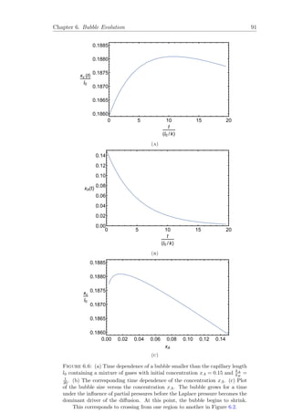
![Chapter 6. Bubble Evolution 92
steeper (i.e. once the bubble shrinks) indicating that the changes in xA with time
become progressively smaller. However, even as the bubble shrinks the change in
concentration remains negative which indicates that once the bubble crosses from
a growing regime to a shrinking regime, it remains in this regime thereafter.
In experiment, it is common practice to enclose the entire system within a finite
box to limit extraneous experimental effects (e.g. evaporation) [65]. The volume of
this reservoir will decrease over time as the bubble grows, providing a mechanism
for equalisation of the partial pressure differences over very long times. However,
this occurs over a significantly longer time than considered in this work and so we
neglect this effect in our analysis.
6.4 Simple Scaling Models for the Evolution of
Ideal, Hemispherical Gas Bubbles Due to
Pressure-induced Gas Diffusion
Bubbles for which the bubble size xc greatly exceeds the capillary length are well
approximated by a hemispherical shape of radius Rc = xc. In this case, it is
straightforward to compute the evolution of bubble size with time analytically,
based on an integration of Fick’s Law (see equations (6.3) and (6.5)), together
with the appropriate expression for the pressure differences. In the following, we
will show how this reproduces the scaling laws found in our simulations for large
bubbles and shown in Figures 6.3 and 6.4 for shrinking and growing bubbles,
respectively.
6.4.1 Case One: Permeability kB
For a hemispherical bubble of radius xc = Rc on a flat surface (or equally a free
spherical bubble), we have the Laplace law ∆p = 4σ
Rc
, Ac = 2πR2
c and V = 2
3
πR3
c
where σ is the surface tension of the liquid films. Inserting these into Fick’s](https://image.slidesharecdn.com/0b1eb23b-c092-4b30-8aa1-2e454aa93edb-160425224409/85/Thesis_Robert_Murtagh_Corrected-106-320.jpg)
![Chapter 6. Bubble Evolution 93
equation (6.3) with Rc(t0) = R0 and integrating we readily obtain
Rc(t)2
= R2
0 −
8σkB
P0
(t − t0). (6.10)
This is indeed the scaling behaviour that we found in our simulations of large
shrinking bubbles in section 6.3.1, Figure 6.3.
6.4.2 Case Two: Permeabilities kB = 0 and kA = 0
Next, we consider the case of a hemispherical bubble on a flat surface containing
two gases with kB and kA kB, respectively.
For a hemispherical bubble we have, again, Ac = 2πR2
c and V = 2
3
πR3
c. Taking
the dominant pressure difference to be due to partial pressure, inserting into (6.5)
and integrating leads to
Rc(t)4
= R4
0 +
6kBVA
π
(t − t0), (6.11)
where VA is the volume of gas B in the bubble.
This is indeed the scaling law for large bubbles as found in our simulations (see
Figure 6.4). A more detailed derivation for both of these power laws is given in
Appendix H.
6.5 Experimental Procedure and Results
In addition to the theoretical and simulation studies described above, experimental
studies were carried out by A. Meagher to illustrate the growth law of a single,
stabilised bubble at a liquid surface containing a mixture of nitrogen gas (N2) and
the compound perfluorohexane (PFH)[66].](https://image.slidesharecdn.com/0b1eb23b-c092-4b30-8aa1-2e454aa93edb-160425224409/85/Thesis_Robert_Murtagh_Corrected-107-320.jpg)
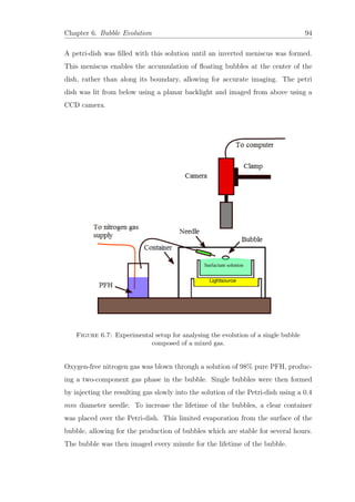
![Chapter 6. Bubble Evolution 95
Using ImageJ [68], the experimental images were binarised and the resulting bub-
ble diameter (measured as twice xc) determined using the watershed transforma-
tion [68, 69]. Due to internal reflection within the bubble bulk, a 10 % reduction
was taken into account for the measured values of the bubble size xc [69]. Typical
expansion data for a single bubble is shown in Figure 6.8.
Figure 6.8: Evolution of the bubble size xc with time t. The data was fitted
between 580s where xc ≈ l0 and 3500s using the function xc(t) = (a+bt)c, with
a calculated exponent of c = 0.28 ± 0.01. Deviations from this power-law fit are
seen at longer times.
The smooth growth of the bubble was tracked for over an hour. During this time, it
was found the bubble size xc increased by a factor of 4. Fitted to the experimental
data was an equation of the form xc(t) = (a + bt)c
in order to determine the
validity of the theoretical prediction as seen in equation (6.11).
Figure 6.8 shows the result of one such experiment. It was found that the growth
of the bubble size xc was well approximated by a power law with an exponent of
c = 0.28±0.01 in the limited range 580s to 3500s, slightly exceeding the ideal case
of c = 0.25. In the mean of seven experiments, where the lifetime of the bubble](https://image.slidesharecdn.com/0b1eb23b-c092-4b30-8aa1-2e454aa93edb-160425224409/85/Thesis_Robert_Murtagh_Corrected-109-320.jpg)

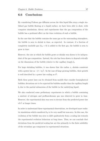


![Chapter 7. Conclusion and Outlook 100
Figure 7.1: Schematic diagram of an interface between two bubbles A and
B which is curved when there is an internal pressure difference between the
bubbles. In general, the curvature is measured by the two principal radii of
curvature R1 and R2 (which are perpendicular to each other) which are related
to the pressure difference via the Young-Laplace law (see Section 1.2). For
rotationally symmetric films, the radii of curvature are the same and denoted
by Rc. This image has been reproduced from [3].
kept constant in our previous analyses, however, is the curvature of the bubble-
bubble contacts; we have only considered ordered foam in which the pressure in all
of the bubbles is the same. In this case, the approximation of rotational symmetry
inherent in our model, implies a planar, circular interface between neighbouring
bubbles.
Here we extend the cone model to deal with the case of bubbles with differing
internal pressures. In general, this leads to a curvature of the interface which is
described by two principal radii of curvature, as shown in Figure 7.1 [3]. Using](https://image.slidesharecdn.com/0b1eb23b-c092-4b30-8aa1-2e454aa93edb-160425224409/85/Thesis_Robert_Murtagh_Corrected-114-320.jpg)
![Chapter 7. Conclusion and Outlook 101
rotational symmetry, however, the picture is simpler as the interface is a spherical
cap with a single radius of curvature Rc. While the Weaire-Phelan structure (see
1.3(b)) is a famous example of a monodisperse foam where the individual bubbles
have different pressures [23], it is more common for differing internal pressures to
arise in polydisperse foam. As we hinted in Section 1.6, a difference in bubble
size will have an effect on the bubble-bubble interaction because the deformation
ξ will be different for the larger and the smaller bubbles for the same contact size.
At this point, we note that the mathematical derivation of the excess energy ε
and ξ (for both the larger and smaller bubbles) for curved contacts is similar in
style to that outlined in Appendix A for the Z-cone model. However, the presence
of curved contacts introduces some additional complications which are relevant to
the details of our Euler-Lagrange formalism and lead to somewhat lengthy analytic
expressions for ε and ξ. Thus, they are left to Appendix C.
In both the original Z-cone model and its extension to the Kelvin cell, we rep-
resented the presence of equal-sized neighbouring bubbles as flat contacts (see
Figure 2.3) compressing a bubble from each of Z directions. For simplicity, we
shall begin by looking at the case of a small bubble confined by larger bubbles. A
convenient way to think about curved contacts is to simply replace the flat plates
with spherical boundaries. A representation of this, for the case of Z = 2, is shown
in Figure 7.2.
(a) (b)
Figure 7.2: We investigate the case of Z = 2 contacts by using spherical, rather
than flat, boundaries to confine the bubble, appropriate when the pressure of
neighbouring bubbles is different from that of the central one.](https://image.slidesharecdn.com/0b1eb23b-c092-4b30-8aa1-2e454aa93edb-160425224409/85/Thesis_Robert_Murtagh_Corrected-115-320.jpg)
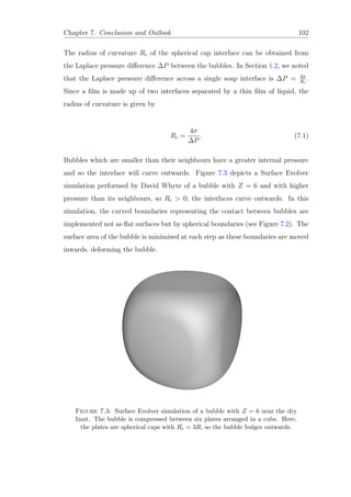
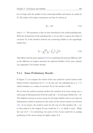

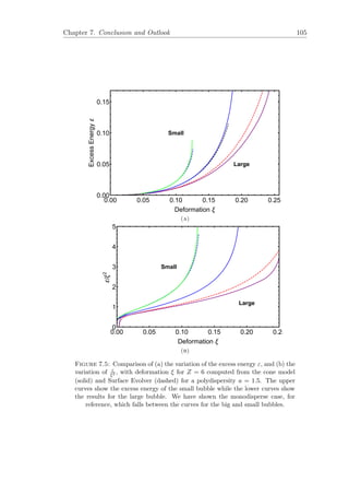
![Chapter 7. Conclusion and Outlook 106
The polydispersity a of the system controls the degree to which the excess energy
for the large and small bubble deviates from the monodisperse case. This is shown
in Figure 7.6 for the case of Z = 6. As the polydispersity increases, the excess
energies for the large and small bubbles are observed to deviate more and more
from the monodisperse case.
The success of this extension to the cone model could instigate further applications
of the cone model to the case of periodic bi-disperse structures, for example in the
sodium chloride lattice.
7.2 Cone Model for Bubble Clusters
In extending the cone model to more and more general cases, we have yet to
mention bubble clusters or adherence to Plateau’s laws, in particular the 120◦
meeting angle for three soap films. The reason for this is simply that we have
always been considering the case of a bubble in the bulk of a liquid foam. In the
future, we hope to extend this model to clusters of bubbles [70–72] for which we
will certainly need to take into account this meeting condition [73].
While the geometry of many bubble clusters, such as those considered by Cox
and Graner [70], remains very much part of future work, we present a preliminary
extension of the Z-cone model to describe the far simpler two-bubble clusters,
otherwise known as bubble chains, considered by Bohn [73] which consist of two
soap bubbles which are strained between two parallel surfaces. While Bohn showed
that there are several configurations possible for these two bubble clusters which
transition into each other as a function of the separation of the plates, we restrict
ourselves to considering the chain arrangement in which the two bubbles adhere
to separate plates along a contact line (equivalent to r(0) for Z = 2, see Figure
2.3) and form a contact which is parallel to the plates. In contrast to our previous
extensions of the Z-cone model, adapting the existing Z-cone model for such a
bubble chain is relatively simple, requiring only two small changes to the derivation
of Z-cone model given in Appendix A.](https://image.slidesharecdn.com/0b1eb23b-c092-4b30-8aa1-2e454aa93edb-160425224409/85/Thesis_Robert_Murtagh_Corrected-120-320.jpg)

![Chapter 7. Conclusion and Outlook 108
Firstly, we must replace the infinity in the first of the boundary conditions, equa-
tion (A.7), with the cotangent of an appropriate angle to impose the 120◦
angle
condition at the edge of the contact. Secondly, we must remember that for these
clusters, the free surface of the bubble is not a single surfactant interface separat-
ing gas in the bubble from liquid outside but a true film consisting of two such
interfaces. This is simply done by doubling the contribution of the free surface to
the total area of the bubble, equation (A.22).
7.2.1 Preliminary Results: Two-Bubble Chains
In this section, we present a number of preliminary results for the same two-bubble
chain considered by Bohn [73], where the each bubble is initially a hemisphere
with radius R0 = 1. Each of these results compares our adapted Z-cone model
for bubble clusters with the equivalent system for the original Z-cone model. In
doing so, we clearly illustrate the effect of imposing the 120◦
angle condition in
our model.
In Figure 7.7, we show the variation of the radii δ and r(0) with distance between
the bubble centres s (i.e. the separation of the parallel plates in experiment) for the
two models. The reason to use s instead of deformation ξ is that the imposition
of the angle condition allows for negative deformations, which is not a natural
concept. Also, it is easy to compare our results directly with the experimental
results of Bohn [73].
We see that for true bubble clusters, the contact between the bubbles is non-zero
for distances greater than s = 2 (when the bubbles are hemispheres with a point
contact). This agrees with the experimental results of Bohn [73] who observed that
once a contact was formed between the bubbles by bring them into contact, and
that this contact persisted as the plates were then separated beyond the reference
position of s = 2. As this behaviour is not observed for the original Z-cone model,
we conclude that this effect is a direct result of the angle condition.](https://image.slidesharecdn.com/0b1eb23b-c092-4b30-8aa1-2e454aa93edb-160425224409/85/Thesis_Robert_Murtagh_Corrected-122-320.jpg)
![Chapter 7. Conclusion and Outlook 109
1.0 1.5 2.0 2.5
0.0
0.2
0.4
0.6
0.8
1.0
1.2
Distance Between Bubble Centres s
R[D]
δ
r(0)
Figure 7.7: Comparison of the radius of the contact (upper) and of the film
(lower), separating two hemispherical bubbles in a two-bubble cluster from the
Z-cone model. The solid lines represent a two-bubble cluster with a 120◦ an-
gle condition, as shown in the inset. The dashed lines are the corresponding
quantities for the original Z-cone model (see Chapter 2).
0.0 0.5 1.0 1.5 2.0 2.5
-0.1
0.0
0.1
0.2
0.3
0.4
Distance Between Bubble Centres s
ExcessEnergyε
Figure 7.8: Comparison of the variation of excess energy ε with distance be-
tween bubble centres s for the two models. We see that the Z-cone model (solid)
is well-behaved as the bubble as brought into contact, while the adapted model
for bubble clusters (solid) shows a variety of additional features. In particular,
we observe that the excess energy is double-valued for s > 2. Naturally, this is
unphysical and the experimental system is observed to occupy the lowest energy
configuration for each s.
Figure 7.8 shows a comparison between the excess energies ε for the two models. As](https://image.slidesharecdn.com/0b1eb23b-c092-4b30-8aa1-2e454aa93edb-160425224409/85/Thesis_Robert_Murtagh_Corrected-123-320.jpg)
![Chapter 7. Conclusion and Outlook 110
we expect, the excess energy for the original Z-cone model increases monotonically
as the bubbles are brought into contact.
However, the variation of the excess energy is more complicated for the bubble
cluster. We observe that there are two values of ε for each values of s 2. The
upper branch of the dashed curve corresponds to an unstable configuration which
is not realised experimentally as bubbles will always jump to the lowest energy
configuration available.
While the work presented here is still in its infancy, the successful replication of
experimental results could spur further development of the model to more com-
plicated bubble clusters [70] in the future.](https://image.slidesharecdn.com/0b1eb23b-c092-4b30-8aa1-2e454aa93edb-160425224409/85/Thesis_Robert_Murtagh_Corrected-124-320.jpg)

![Appendix A. Z-Cone Model Derivation 112
The total surface area A, per contact Z, of our bubble can be written as
A = Aδ + 2π
h
0
r(z) 1 +
dr(z)
dz
2
dz, (A.1)
where Aδ is the surface area of the contact. In the case of flat contacts Aδ = πδ2
.
The second term in this equation is the general expression for the surface area
(of revolution) of any curve given by r(z) [38]. The volume V under this curve is
given by
V = π
h
0
r(z)2
dz +
πr(0)3
cot θ
3
. (A.2)
Minimising this surface area under the constraint of constant volume is the subject
of the calculus of variations and requires the Euler-Lagrange formalism [38]. In
general, the Euler-Lagrange equation is given by
dL r(z), dr(z)
dz
, z
dr(z)
−
d
dz
dL r(z), dr(z)
dz
, z
d dr(z)
dz
= 0. (A.3)
Fortunately, the Lagrangian function L that we consider does not depend explicitly
on the coordinate z
L r(z),
dr(z)
dz
= 2r(z) 1 +
dr(z)
dz
2
− λr(z)2
. (A.4)
In this special case, we can make a significant simplification of our minimisation
problem by using an integrated form of the Euler-Lagrange equation (equation
(A.5)) whose derivation we give here](https://image.slidesharecdn.com/0b1eb23b-c092-4b30-8aa1-2e454aa93edb-160425224409/85/Thesis_Robert_Murtagh_Corrected-126-320.jpg)
![Appendix A. Z-Cone Model Derivation 113
dL
dr(z)
dr(z) −
d
dz
dL
d dr(z)
dz
dr(z) = 0 dr(z),
C + L −
d
dz
dL
d dr(z)
dz
dr(z) = 0,
L −
d
dr(z)
dr(z)
dz
dL
d dr(z)
dz
dr(z) = −C,
L − d
dr(z)
dz
dL
d dr(z)
dz
= −C,
∴
dr(z)
dz
dL
d dr(z)
dz
− L = C, (A.5)
where C is an unknown integration constant. Equation (A.5) is known as Bel-
trami’s Identity and is at the heart of the calculus of variations [38]. For example,
it is used instead of the standard Euler-Lagrange equation (equation (A.3)) in
solving the brachistochrone (“shortest-time”) problem [74]; this classic problem,
first proposed by Johann Bernouilli in 1696, involves finding “the curve joining two
points such that a bead starting from rest at the higher point will slide without
friction along the curve and reach the lower point in the shortest possible time”.
[74].
Inserting our Lagrangian function and its derivative into Beltrami’s Identity we
obtain
−
2r(z)
1 + dr(z)
dz
2
+ λr(z)2
= C. (A.6)](https://image.slidesharecdn.com/0b1eb23b-c092-4b30-8aa1-2e454aa93edb-160425224409/85/Thesis_Robert_Murtagh_Corrected-127-320.jpg)

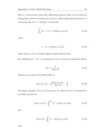

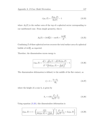

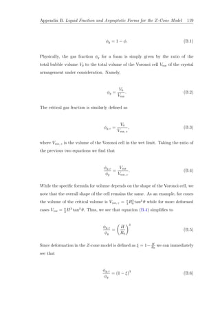


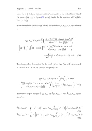


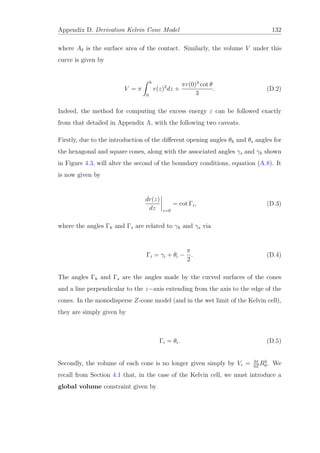
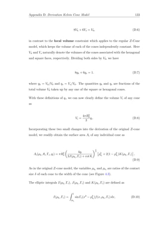

![Appendix D. Derivation Kelvin Cone Model 135
We have used the fact that the Voronoi cell which surrounds each of the cones
in our geometric construction is a right-circular cone, with a volume given by
Vi = π
3
H3
i tan2
θi.
Up to this point, we have largely considered the hexagonal and square cones in
isolation, connected only by the total volume constraint. However, for these cones
to constitute a realistic model of a foam, we require the two types of cone to have
a common slant height rs, for both the deformable cones and the Voronoi cones.
Furthermore, we know that in the exact Kelvin cell, the ratio of distances Hh
Hs
from
the centre of the bubble to each of the faces maintains a constant ratio of
√
3
2
, at
least for the isotropic deformation which we consider here. Combining these two
ideas, we find that for the cone model, the ratio of distances to the faces of the
Kelvin cell is slightly different from stated above. It is given by
⇒
Hh
cos θh
=
Hs
cos θs
= ν = 0.864434. (D.16)
Inserting this relation, equation (D.16) into equation (D.15), along with height Hh
of the hexagonal cone given by
Hh = R0
4qh
3J(ρδh
, Γh) + cot θh
1
3
[I(ρδh
, Γh) + cot θh] , (D.17)
and simplifying, we obtain the liquid fraction φ = 1−φg for the cone model applied
to the Kelvin cell as
φ(ρδh
, θh, θs, Γh, qh) = 1 −
3J(ρδh
, Γh) + cot θh
2qh [I(ρδh
, Γh) + cot θh]3
4 tan2
θh + 3
υ3 tan2
θs
.
(D.18)
The arguments presented here are general, and can be applied to describe a foam
structure with more than two different types of cones. For more than two different
types of cones, we simply need to specify the ratios of distances νi to each of the](https://image.slidesharecdn.com/0b1eb23b-c092-4b30-8aa1-2e454aa93edb-160425224409/85/Thesis_Robert_Murtagh_Corrected-149-320.jpg)
![Appendix D. Derivation Kelvin Cone Model 136
different sets of faces, taking the nearest neighbours as a reference. Indicating the
nearest neighbour contacts by the the index nn we have
νi =
Hnn
Hi
=
cos θnn
cos θi
. (D.19)
Thus, the liquid fraction can be expressed for any number of cones by
φ(ρδnn , θnn, Γnn, qnn, θi, Zi, νi) = 1 −
3J(ρδnn , Γnn) + cot θnn
qnn [I(ρδnn , Γnn) + cot θnn]3 .
1
i
Zi
ν3
i
tan2
θi
.
(D.20)
This has the form φ = 1 − G(ρδ1 , θ1, Γ1, q1)M(θi, Zi, νi) where G is a function of
the nearest neighbour variables only while M encodes the details of the structure.
D.3 Pressure pi
We stated in Chapter 4, that in order to provide a sufficient number of constraints
to uniquely determine all of the variables involved in the extended cone model, we
need to consider the internal pressure of our bubble.
The internal pressure of a bubble is higher than the atmospheric pressure, giving
rise to the curvature of the surface. In the cone model, the pressure pi in each of
the cones must be equal so we will only discuss a single cone in what follows. In
order to calculate the pressure pi, we rely on a simple thermodynamic argument
regarding the work done to increase the volume of the cone while keeping the size
of the contact δi constant.
We begin by considering the volume of a cone as the sum of two parts, Vi and V ∗
i ,
such that
Vi = Vi + V ∗
i . (D.21)](https://image.slidesharecdn.com/0b1eb23b-c092-4b30-8aa1-2e454aa93edb-160425224409/85/Thesis_Robert_Murtagh_Corrected-150-320.jpg)


![Appendix E. Estimation of Dry Kelvin 142
Kusner and Sullivan sketch the computation of a lower bound for the energy of a
Kelvin cell [75] using a similar argument to above, resulting in A/A0 1.0954.](https://image.slidesharecdn.com/0b1eb23b-c092-4b30-8aa1-2e454aa93edb-160425224409/85/Thesis_Robert_Murtagh_Corrected-156-320.jpg)
![Appendix F
Simulating Bubbles in a Confined
Geometry with the Surface
Evolver
The Surface Evolver software [18] developed by Prof. Kenneth Brakke is widely
used in computational modelling of surfaces driven by surface tension, such as
soap bubbles, subject to a variety of constraints. We have made use of the Surface
Evolver to evaluate the excess energy ε of a single bubble in an ordered foam to
provide a comparison with the results obtained from the cone model. This was
necessary because of the inherent experimental difficulties of stabilising, imaging
and measuring the surface area of a bubble in the bulk of a foam, particularly close
to the wet limit. We wish to acknowledge the help of David Whyte in particular
and also Steven Tobin for help, with regard to performing these simulations.
In simplest terms, the Surface Evolver works by representing a continuous surface,
such as a liquid film, approximately as a series of points joined together by directed
straight edges forming a mesh of triangular facets. A normal vector is assigned
to each of the facets to specify whether it faces inwards or outwards. This is
important because we define a body such as a bubble as a list of facets which all
point in the same direction.
143](https://image.slidesharecdn.com/0b1eb23b-c092-4b30-8aa1-2e454aa93edb-160425224409/85/Thesis_Robert_Murtagh_Corrected-157-320.jpg)
![Appendix F. Surface Evolver 144
Once a bubble is defined in this way, it is possible to constrain it to have a certain
fixed volume. The success of this approach can be seen in the example of a spherical
bubble which is initially specified as a crude cubic lattice of points connected by
edges. Once this tessellation has been defined, its correspondence to a sphere is
improved by further subdividing into smaller triangles and by allowing the vertices
to move in order to minimise the total surface area. This minimisation is done
here using the method of conjugate gradient descent [18]. By implementing a series
of refinements of the tessellation and minimisation steps, the cube becomes more
rounded and we obtain a better and better approximation of a spherical bubble.
Increasing the number of tessellations significantly increases the memory required
to store the configuration and slows down the minimisation procedure and the
degree of refinement used must be tailored to the accuracy required.
To simulate the contact of such a spherical bubble with Z neighbouring bubbles
in a crystalline arrangement, we define a series of planes in the direction of the
neighbouring bubbles. These planes are treated as impenetrable barriers, with the
bubble surface constrained to lie strictly within this arrangement of planes. These
planes are initially defined to be situated slightly beyond the edge of the bubble
and the deformation proceeds by moving the planes steadily closer to the bubble
in a series of steps. Each time the bounding planes are moved in, the surface of
the bubble is refined and minimised with the final value of the surface area A
being stored before moving on to the next stage. This method was also used for
comparison with the curved contact cone model of Chapter 7 with the flat planes
being replaced by curved planes whose curvature was specified to match the radius
of curvature of the contact.
While the deformation ξ is clearly defined at each time step by the position of the
planes, the excess energy ε = A/A0 −1 is more subtle. This is due to the fact that
it depends crucially on the value of A0, the surface area of the initial spherical
bubble. For accurate comparison with the cone model, which is only limited by
the accuracy with which the numerical integrals can be performed, the degree of
tessellation in this case needs to be high (we refined and minimised at least five
times in each of our simulations).](https://image.slidesharecdn.com/0b1eb23b-c092-4b30-8aa1-2e454aa93edb-160425224409/85/Thesis_Robert_Murtagh_Corrected-158-320.jpg)
![Appendix F. Surface Evolver 145
Figure F.1: The equilibrium structure for a Kelvin foam, including all surfaces
within the conventional cell. The 1 1 1 contact faces are shown in red, and the
1 0 0 faces in blue. This is built, exploiting the reflectional symmetries, from
a representative cell one eight the size of this cell. Indeed, the full foam can be
built from reflected and translated copies of such a representative cell.
The Kelvin foam consists of repeated translated copies of the conventional bcc for
a foam shown in Figure F.1. The procedure for simulating this Kelvin cell with
the Surface Evolver was different to that for the Z-cone model. For simplicity, we
can exploit some of the symmetries of the conventional cell; namely, reflectional
symmetry in the x, y and z directions. Brakke and Sullivan [76] exploit even more
symmetries to yield a minimal representation of the full dry Kelvin foam. Hence
we arrive at a reduced cell, which has one eighth of the volume of the conventional
cell, and is composed of a cube containing one eighth of a bubble at each of two
opposite corners. This increases the speed of computation considerably.
We begin with a very roughly triangulated approximation of the configuration in
Figure F.1, with appropriate film edges constrained to lie within the faces of the](https://image.slidesharecdn.com/0b1eb23b-c092-4b30-8aa1-2e454aa93edb-160425224409/85/Thesis_Robert_Murtagh_Corrected-159-320.jpg)

![Appendix G
Computation of the Bubble Shape
The purpose of this appendix is to briefly outline how the precise shape of a
single bubble at a liquid surface (see Figure 6.1) is calculated, using an algorithm
developed by Princen [57]. This procedure forms an integral part of the simulations
of gas diffusion in bubbles which we discussed in Chapter 6.
Figure G.1: Schematic 2-D cross-section of a gas bubble (Phase 1) at the
surface of a liquid (Phase 2). The point (xc, zc) marks a ring of contact above
which the bubble is in contact with the gaseous atmosphere. L represents the
height of the liquid surface above the bottom of the bubble while φc is the angle
made between the normal at (xc, zc) and the negative z-direction. This figure
is reproduced from Princen [57].
147](https://image.slidesharecdn.com/0b1eb23b-c092-4b30-8aa1-2e454aa93edb-160425224409/85/Thesis_Robert_Murtagh_Corrected-161-320.jpg)
![Appendix G. Bubble Shape Calculation 148
The 2D cross-section of a surface bubble, represented schematically in Figure G.1,
is described by the following three shape equations [57]:
1
R1
+
1
R2
= cz +
2
b
, (interface between bubble and bulk-liquid) (G.1)
1
R1
+
1
R2
=
2
Rc
, (spherical cap) (G.2)
1
R1
+
1
R2
= c(z − L), (distorted liquid surface). (G.3)
As we described in Section 6.1, above the point (xc, zc) the bubble shape is a
spherical cap with a radius of curvature Rc. The other interfaces are more com-
plicated, however, with the radii of curvature, R1 and R2, of each of the interfaces
given by
1
R1
=
d2z
dx2
[1 + (dz
dx
)2]3/2
(G.4)
and
1
R2
=
dz
dx
x[1 + (dz
dx
)2]1/2
. (G.5)
The radius of curvature at the bottom of the bubble is given by b and c is given
by
c =
1
l2
0
=
∆ρg
σ
, (G.6)
where l0 is the capillary length (see equation (6.1)). L is the height of the flat
liquid surface above the bottom of the bubble and is related to our other simulation
parameters by the relation L = 2
c
( 2
Rc
− 1
b
).](https://image.slidesharecdn.com/0b1eb23b-c092-4b30-8aa1-2e454aa93edb-160425224409/85/Thesis_Robert_Murtagh_Corrected-162-320.jpg)
![Appendix G. Bubble Shape Calculation 149
The algorithm for solving this system for the shape of the bubble begins by spec-
ifying the volume of the initial bubble. The radius of curvature Rc of the bulk
interface is given by Rc = xc
sin φc
[57], where xc is the experimentally observed bub-
ble radius (viewed from above) and φc is the angle made between the normal at
(xc, zc) and the negative z-direction.
The spherical cap and bulk-liquid interfaces must have a common slope of tan φc
at the critical point (xc, zc). Utilising this condition, the system of equations is
then solved (in our case using the ode45 equation solver method from Matlab.)
for a value of φc satisfying the boundary conditions of total bubble volume and
slope matching at the intersection point. We obtain the value of the critical point
(xc, zc), the radius of curvature Rc as well as the area of permeation Ac of the bulk
interfacial film. This completely specifies the shape of the bubble for this volume.
Thus we can apply an appropriate form of Fick’s Law (see Section 6.3) to allows
us to obtain a new bubble volume and the process is repeated.](https://image.slidesharecdn.com/0b1eb23b-c092-4b30-8aa1-2e454aa93edb-160425224409/85/Thesis_Robert_Murtagh_Corrected-163-320.jpg)
![Appendix H
Gas Diffusion in Bubbles
In this appendix, we provide derivations for the key analytical results presented in
our discussion of the diffusion characteristics of a single gas bubble in Chapter 6.
As we did in Chapter 6, we will differentiate between bubbles containing a single,
soluble gas of permeability kB and bubbles containing a mixture of two gases (A
and B) with different permeabilities kA and kB. We shall refer to these two cases
as Case One and Case Two, respectively (see Section 6.2).
H.1 Boundary Between Growing and Shrinking
We recall from Chapter 6 that the diffusion of gas between bubbles proceeds
according to pressure gradients, with gas flowing from regions of higher pressure
to lower pressure according to Fick’s First Law of Diffusion [59]. The total gas
pressure pg in a single bubble is higher than the atmospheric pressure P0 by an
amount ∆p equal to the Laplace pressure
∆p = pg − P0 =
4σ
Rc
, (H.1)
where Rc is the radius of curvature of the diffusing film.
150](https://image.slidesharecdn.com/0b1eb23b-c092-4b30-8aa1-2e454aa93edb-160425224409/85/Thesis_Robert_Murtagh_Corrected-164-320.jpg)


![Bibliography
[1] G. Johansson and R. J. Pugh. The influence of particle size and hydropho-
bicity on the stability of mineralized froths. International Journal of Mineral
Processing, 34(1-2):1–21, 1992.
[2] D. Weaire and S. Hutzler. The Physics of Foams. Oxford University Press,
Oxford, 1999.
[3] I. Cantat, S. Cohen-Addad, F. Elias, F. Graner, R. H¨ohler, O. Pitois,
F. Rouyer, and A. Saint-Jalmes. Les mousses – Structure et dynamique.
´Editions Belin, Paris, 2010.
[4] H. M. Princen. Rheology of Foams and Highly Concentrated Emulsions I.
Elastic Properties and Yield Stress of a Cylindrical Model System. J. Colloid
Interface Sci., 91:160–175, 1983.
[5] H. M. Princen and A. D. Kiss. Osmotic pressure of foams and highly con-
centrated emulsions. 2. Determination from the variation in volume fraction
with height in an equilibrated column. Langmuir, 3:36–41, 1987.
[6] S. Tcholakova, N. D. Denkov, K. Golemanov, K. P. Ananthapadmanabhan,
and A. Lips. Theoretical model of viscous friction inside steadily sheared
foams and concentrated emulsions. Physical Review E, 78:011405, 2008.
[7] J. F. Sadoc and N. Rivier (eds.). Foams and Emulsions, Proceedings of the
NATO Advanced Study Institute on Foams and Emulsions, Emulsions and
Cellular Materials, Carg`ese, Corsica, 12-24 May, 1997. Kluwer Academic
Publishers, Dordrecht,Boston,London, 1999.
158](https://image.slidesharecdn.com/0b1eb23b-c092-4b30-8aa1-2e454aa93edb-160425224409/85/Thesis_Robert_Murtagh_Corrected-172-320.jpg)
![Bibliography 159
[8] T. Aste and D. Weaire. The Pursuit of Perfect Packing (2nd edition). Taylor
& Francis, London, 2008.
[9] D. Weaire, V. Langlois, M. Saadatfar, and S. Hutzler. Foam as granular
matter. In Di Matteo T. Aste T and Tordesillas A, editors, Granular and
Complex Materials, World Scientific Lecture Notes in Complex Systems, vol-
ume 8, pages 1–26, New Jersey, 2007. World Scientific Publishing.
[10] J. A. F. Plateau. Statique Exp´erimentale et Th´eorique des Liquides soumis
aux seules Forces Mol´eculaires. Gauthier-Villars, Paris, 1873.
[11] J. E. Taylor. The Structure of Singularities in Soap-Bubble-Like and Soap-
Film-Like Minimal Surfaces. The Annals of Mathematics, 103(3):489, 1976.
[12] R. H¨ohler, Y. Y. C. Sang, S. Lorenceau, and S. Cohen-Addad. Osmotic
pressure and structures of monodisperse ordered foam. Langmuir, 24:418–
425, 2008.
[13] D. Weaire and R. Phelan. A Counter-example to Kelvin’s Conjecture on
Minimal-Surfaces. Philosophical Magazine Letters, 69(2):107–110, 1994.
[14] R. Gabbrielli, A. J. Meagher, D. Weaire, K. A. Brakke, and S. Hutzler. An ex-
perimental realization of the Weaire–Phelan structure in monodisperse liquid
foam. Philosophical Magazine Letters, 92(1):1–6, 2012.
[15] A. M. Ganan-Calvo. Perfectly monodisperse microbubbling by capillary flow
focusing: An alternate physical description and universal scaling. Physical
Review E, 69(2), 2004.
[16] W. Drenckhan, S. J. Cox, G. Delaney, H. Holste, D. Weaire, and N. Kern.
Rheology of ordered foams - on the way to Discrete Microfluidics. Colloids and
Surfaces a-Physicochemical and Engineering Aspects, 263(1-3):52–64, 2005.
[17] A. J. Meagher, D. Whyte, J. Banhart, S. Hutzler, D. Weaire, and F. Garc´ıa-
Moreno. Slow crystallisation of a monodisperse foam stabilised against coars-
ening. Soft Matter, 11(23):4710–4716, 2015.](https://image.slidesharecdn.com/0b1eb23b-c092-4b30-8aa1-2e454aa93edb-160425224409/85/Thesis_Robert_Murtagh_Corrected-173-320.jpg)
![Bibliography 160
[18] K. A. Brakke. The Surface Evolver. Experimental Mathematics, 1:141–165,
1992. URL http://www.susqu.edu/facstaff/b/brakke/evolver/.
[19] J. A. F. Plateau. Statique Exp´erimentale et Th´eorique des Liquides soumis
aux seules Forces Mol´eculaires. Gauthier-Villars, Paris, 1873.
[20] H. M. Princen and P. Levinson. The surface area of Kelvin’s minimal
tetrakaidecahedron: The ideal foam cell (?). Journal of Colloid and Interface
Science, 120(1):172–175, November 1987.
[21] A. van der Net, G. W. Delaney, W. Drenckhan, D. Weaire, and S. Hutzler.
Crystalline arrangements of microbubbles in monodisperse foams. Colloids
and Surfaces A: Physicochemical and Engineering Aspects, 309:117–124, 2007.
[22] M. Saadatfar, J. Barry, D. Weaire, and S. Hutzler. Ordered cylindrical foam
structures with internal bubbles. Philosophical Magazine Letters,, 88:661–668,
2008.
[23] R. Phelan. Foam structure and properties. PhD thesis, Trinity College Dublin,
1996.
[24] D. Weaire and S. Hutzler. The Physics of Foams. Oxford University Press,
Oxford, 1999.
[25] S. J. Cox. A viscous froth model for dry foams in the surface evolver. Coll.
Surf. A, 263:81–89, 2005.
[26] H. M. Princen and A. D. Kiss. Osmotic pressure of foams and highly con-
centrated emulsions. 2. Determination from the variation in volume fraction
with height in an equilibrated column. Langmuir, 3:36–41, 1987.
[27] M. D. Lacasse, G. S. Grest, and D. Levine. Deformation of small compressed
droplets. Physical Review E, 54(5):5436–5446, 1996.
[28] D. J. Durian. Foam mechanics at the bubble scale. Phys. Rev. Lett., 75:
4780–4783, 1995.](https://image.slidesharecdn.com/0b1eb23b-c092-4b30-8aa1-2e454aa93edb-160425224409/85/Thesis_Robert_Murtagh_Corrected-174-320.jpg)
![Bibliography 161
[29] V. J. Langlois, S. Hutzler, and D. Weaire. Rheological properties of the soft
disk model of 2D foams. Phys. Rev. E, 78:021401, 2008.
[30] P. J. Hoogerbrugge and J. M. V. A. Koelman. Simulating microscopic hydro-
dynamic phenomena with dissipative particle dynamics. Europhysics Letters,
19(3):155–160, 1992.
[31] E. Moeendarbary, T. Y. NG, and M. Zangeneh. Dissipative particle dynam-
ics: Introduction, methodology and complex fluid applications - A review.
International Journal of Applied Mathematics, 1(4):737–763, 2009.
[32] N. D. Denkov, V. Subramanian, D. Gurovich, and A. Lips. Wall slip and
viscous dissipation in sheared foams: Effect of surface mobility. Colloids
Surf. A, 263:129–145, 2005.
[33] P. Doshi, I. Cohen, W. W. Zhang, M. Siegel, P. Howell, O. A. Basaran, and
S. R. Nagel. Persistence of memory in drop breakup: The breakdown of
universality. Science, 302(5648):1185–1188, 2003.
[34] A. M. Ganan-Calvo and J. M. Gordillo. Perfectly monodisperse microbub-
bling by capillary flow focusing. Physical Review Letters, 87(27):274501, 2001.
[35] G. Katgert, B. P. Tighe, M. E. M¨obius, and M. van Hecke. Couette flow of
two-dimensional foams. Europhysics Letters, 90:54002 (6pp), 2010.
[36] A. Wyn, I. T. Davies, and S. J. Cox. Simulations of two-dimensional foam
rheology: localization in linear Couette flow and the interaction of settling
discs. Euro. Phys. J. E, 26:81–89, 2008.
[37] M. B. Sexton, M. E. M¨obius, and S. Hutzler. Bubble dynamics and rheology
in sheared two-dimensional foams. Soft Matter, 7(23):11252, 2011.
[38] L. D. Landau and E. M. Lifshitz. Mechanics. Course of theoretical physics
Vol 1. Elsevier, Butterworth Heinemann, Amsterdam [u.a], 3. ed., reprinted
edition, 2007. ISBN 978-0-7506-2896-9.
[39] D. C. Morse and T. A. Witten. Droplet elasticity in weakly compressed
emulsions. Europhysics Letters, 22:549, June 1993.](https://image.slidesharecdn.com/0b1eb23b-c092-4b30-8aa1-2e454aa93edb-160425224409/85/Thesis_Robert_Murtagh_Corrected-175-320.jpg)
![Bibliography 162
[40] W. H. Press, B. P. Flannery, S. A. Teukolsky, and W. T. Vetterling. Numerical
Recipes in C : The Art of Scientific Computing. Cambridge University Press,
1992. ISBN 0-521-43108-5.
[41] S. Hutzler, R. P. Murtagh, D. Whyte, S. T. Tobin, and D. Weaire. Z-cone
model for the energy of an ordered foam. Soft Matter, 10(36):7103–7108,
2014.
[42] C. B. O’Donovan, E. I. Corwin, and M. A. M¨obius. Mean-field granocen-
tric approach in 2d and 3d polydisperse, frictionless packings. Philosophical
Magazine, 93:4030–4056, 2013.
[43] J. M. Ziman. Approximate Calculation of the Anisotropy of the Relaxation
Time of the Conduction Electrons in the Noble Metals. Physical Review, 121
(5):1320–1324, 1961.
[44] M. van Hecke. Jamming of soft particles: geometry, mechanics, scaling and
isostaticity. J. Phys.: Condens. Matter, 22:033101 (24pp), 2010.
[45] Armando Maestro, Wiebke Drenckhan, Emmanuelle Rio, and Reinhard
H¨ohler. Liquid dispersions under gravity: volume fraction profile and osmotic
pressure. Soft Matter, 9(8):2531–2540, 2013.
[46] D. Weaire, editor. The Kelvin problem. Taylor and Francis, London, 1997.
[47] D. Weaire and R. Phelan. A Counter-example to Kelvin’s Conjecture on
Minimal-Surfaces. Philosophical Magazine Letters, 69(2):107–110, 1994.
[48] D. Weaire, N. Pittet, S. Hutzler, and D. Pardal. Steady-state drainage of an
aqueous foam. Phys. Rev. Lett., 71:2670, 1993.
[49] D. Weaire. Structural transformations in foam. Philosophical Magazine Let-
ters, 69(2):99–105, 1994.
[50] D. M. A. Buzza, C.-Y. D. Lu, and M. E. Cates. Linear shear rheology of
incompressible foams. J. Phys. II France, 5:37–52, 1995.](https://image.slidesharecdn.com/0b1eb23b-c092-4b30-8aa1-2e454aa93edb-160425224409/85/Thesis_Robert_Murtagh_Corrected-176-320.jpg)
![Bibliography 163
[51] D. Weaire and V. Pageron. Frustrated froth: Evolution of foam inhibited by
an insoluble gaseous component. Philos. Mag. Lett., 62:417–421, 1990.
[52] F. Gandolfo and H. Rosano. Interbubble gas diffusion and the stability of
foams. J. Colloid Interface Sci., 184:31–36, 1997.
[53] S. A. Koehler, S. Hilgenfeldt, and H. A. Stone. A generalized view of foam
drainage: Experiment and theory. Langmuir, 16:6327–6341, 2000.
[54] M. A. Fortes and A. M. Deus. Expansion of a foam due to absorption of an
outside gas. J. Colloid Interface Sci., 176:248–255, 1995.
[55] J. Stavans. Temporal evolution of two-dimensional drained soap froth. Phys-
ical Review A, 42(8):5049–5051, 1991.
[56] N. Louvet, F. Rouyer, and O. Pitois. Ripening of a draining foam bubble.
Journal of Colloid and Interface Science, 334:82–86, 2009.
[57] H. M. Princen. Shape of a fluid drop at a liquid-liquid interface. Journal of
Colloid Science, 18(2):178–195, 1963.
[58] M.A.C. Teixeira and P.I.C. Teixeira. Contact angle of a hemispherical bubble:
An analytical approach. Journal of Colloid and Interface Science, 338(1):193–
200, 2009.
[59] H. M. Princen and S. G. Mason. Permeability of soap films to gases. Journal
of Colloid Science, 20(4):353–375, 1965.
[60] G. L. Thomas, J. M. Belmonte, F. Graner, J. A. Glazier, and R. M. C.
de Almeida. 3D simulations of wet foam coarsening evidence a self-similar
growth regime. Physical Review Letters, 473:109–114, 2015.
[61] R. M. C. de Almeida F. Graner. I. Fortuna, G. L. Thomas. Growth laws and
self-similar growth regimes of coarsening two-dimensional foams: Transition
from dry to wet limits. Physical Review Letters, 108(24), 2012.
[62] D. Exerowa and P.M. Kruglyakov. Foam and Foam Films: Theory, Experi-
ment, Application. Elsevier Science, 1997.](https://image.slidesharecdn.com/0b1eb23b-c092-4b30-8aa1-2e454aa93edb-160425224409/85/Thesis_Robert_Murtagh_Corrected-177-320.jpg)
![Bibliography 164
[63] A.P. Grinin, F. M. Kuni, and G. Yu. Gor. The rate of nonsteady gas bubble
growth in liquid supersaturated with gas. Journal of Molecular Liquids, 148:
32–34, 2009.
[64] H. M. Princen and S. G. Mason. Shape of a fluid drop at a fluid-liquid
interface .I. extension and test of 2-phase theory. Journal of Colloid Science,
20(2):156–172, 1965.
[65] A. G Brown, W. C. Thuman, and J. W. McBain. Transfer of air through
adsorbed surface films as a factor in foam stability. Journal of Colloid Science,
8:508–519, 1953.
[66] K. Sarkar, A. Katiyar, and P. Jain. Growth and dissolution of an encapsulated
contrast microbubble: Effects of encapsulation permeability. Ultrasound in
Medicine and Biology, 35(8):1385–1396, 2009.
[67] N. D. Denkov, S. Tcholakova, K. Golemanov, K. P. Ananthpadmanabhan,
and A. Lips. The role of surfactant type and bubble surface mobility in foam
rheology. Soft Matter, 5:3389–3408, 2009.
[68] M. D. Abramoff, P. J. Magalhaes, and S. J. Ram. Image processing with
imagej. Biophotonics International, 11(7):36–42, 2004.
[69] A. van der Net, L. Blondel, A. Saugey, and W. Drenckhan. Simulating and
interpretating images of foams with computational ray-tracing techniques.
Colloids and Surfaces A-Physicochemical and Engineering Aspects, 309:159–
176, 2007.
[70] S. J. Cox and F. Graner. Three-dimensional bubble clusters: Shape, packing,
and growth rate. Physical Review E, 69:031409, 2004.
[71] M. F. Vaz and M. A. Fortes. Two-dimensional clusters of identical bubbles.
J. Phys. Condens. Matter, 13:1395–1411, 2001.
[72] T. C. Hales. Historical overview of the Kepler conjecture. Discrete and
computational geometry, 36(1):5–20, 2006.](https://image.slidesharecdn.com/0b1eb23b-c092-4b30-8aa1-2e454aa93edb-160425224409/85/Thesis_Robert_Murtagh_Corrected-178-320.jpg)
![Bibliography 165
[73] S. Bohn. Bubbles under stress. The European Physical Journal E - Soft
Matter, 11(2):177–189, 2003.
[74] C. B. Boyer and U. C. Merzbach. A History of Mathematics (3rd Edition).
John Wiley and Sons, Inc., New Jersey, 2011.
[75] R. Kusner and J. M. Sullivan. Comparing the Weaire-Phelan equal-volume
foam to Kelvin’s foam. Forma, 11(3):233–242, 1996.
[76] K. A. Brakke and J. M. Sullivan. Using Symmetry Features of the Surface
Evolver to Study Foams. In K. Polthier and H. Hege, editors, Mathematics
and Visualization, Berlin, 1997. Springer Verlag.](https://image.slidesharecdn.com/0b1eb23b-c092-4b30-8aa1-2e454aa93edb-160425224409/85/Thesis_Robert_Murtagh_Corrected-179-320.jpg)


