This document is a PhD thesis submitted by Jamie Fleming to the University of Edinburgh. It contains the following key points:
1. The thesis presents the first measurement of the E double-polarisation observable for the γn → K+Σ- reaction using data from CLAS at JLab.
2. It also provides an overview of Jamie's work developing and constructing the scintillating hodoscope for the CLAS12 Forward Tagger detector upgrade at JLab.
3. The thesis contains acknowledgements, an abstract, introduction to hadron spectroscopy and theoretical models, background on kaon photoproduction reactions, and a review of previous experimental data on the topic.


![LIST OF FIGURES
7.10 Momentum vs ∆β distribution (log scale) for K+
(upper) and
π−
(lower) after data corrections. . . . . . . . . . . . . . . . . . 100
7.11 Momentum vs ∆βcorrected distribution (log scale) for K+
(upper)
and π−
(lower) after a further selection cut. . . . . . . . . . . . 101
7.12 Correlated background seen in the neutron mass spectrum,
reconstructed using the missing mass method. . . . . . . . . . 103
7.13 Initial K+
candidates (upper) in comparison to the K+
candi-
dates after selections performed using ∆β and photon timing
(lower). . . . . . . . . . . . . . . . . . . . . . . . . . . . . . . . 104
7.14 Missing mass of K+
π−
vs ‘K+
’π−
, where ‘K+
’ has the PDG
mass of a π+
. The selection cut is shown in red. . . . . . . . . 106
7.15 Missing mass of K+
π−
vs K+
‘π−
’, where ‘π−
’ has the PDG
mass of a K−
. . . . . . . . . . . . . . . . . . . . . . . . . . . . 107
7.16 Missing mass of K+
π−
vs K+
‘π−
’, after the 2D selection cut
has been applied. . . . . . . . . . . . . . . . . . . . . . . . . . 108
7.17 Missing mass of K+
π−
vs ‘K+
’π−
, where ‘K+
’ has the PDG
mass of a p. . . . . . . . . . . . . . . . . . . . . . . . . . . . . 109
7.18 Missing mass of K+
π−
vs ‘K+
’π−
, after the 2D selection cut
has been applied. . . . . . . . . . . . . . . . . . . . . . . . . . 109
7.19 Missing mass spectrum of the K+
, clearly showing the Λ, Σ−
and Σ(1385). . . . . . . . . . . . . . . . . . . . . . . . . . . . . 110
7.20 2D plot of the reconstructed Σ−
[MM(K+
)] vs. the recon-
structed neutron [MM(K+
π−
)]. . . . . . . . . . . . . . . . . . 111
7.21 2D plot of the reconstructed Σ−
vs the reconstructed neutron
after introducing a linear 2D selection cut. Both the Λ and Σ0
peaks are removed, leaving only Σ−
. . . . . . . . . . . . . . . . 112
7.22 Reconstructed neutron using the missing mass technique [MM(K+
π−
)]
after misID selections have been applied. . . . . . . . . . . . . 113
7.23 Reconstructed neutron using the missing mass technique vs
Momentum. The selection cut is shown in red. . . . . . . . . . 114
7.24 Missing mass of the spectator proton, ps, from the missing mass
technique. . . . . . . . . . . . . . . . . . . . . . . . . . . . . . 115
7.25 Missing momentum of the spectator proton, ps. The selection
cut is shown in red. . . . . . . . . . . . . . . . . . . . . . . . . 116
7.26 A typical spectrum of photon energy when using circularly
polarised beam. The selection cut is shown in red. . . . . . . . 117
7.27 K+
z-vertex from the centre of CLAS. The selection cut is
shown in red. . . . . . . . . . . . . . . . . . . . . . . . . . . . . 119
7.28 K+
z vertex from the centre of CLAS, compared with scaled
empty target data. . . . . . . . . . . . . . . . . . . . . . . . . . 120
7.29 K+
polar vs azimuthal angles (log scale). . . . . . . . . . . . . 121
7.30 K+
polar vs azimuthal angles, after the removal of the fiducial
regions around the CLAS sectors (log scale). . . . . . . . . . . 121
xviii](https://image.slidesharecdn.com/6d482e98-273b-437a-88cf-eb4faf084ce1-161109162450/85/thesis-19-320.jpg)
![LIST OF FIGURES
7.31 Events which have been selected, reconstructed as Σ−
, using
the MM(K+
). The selection cut is shown in red. . . . . . . . . 122
7.32 Events which has been selected, reconstructed as Σ−
, where the
final state neutron has been identified. . . . . . . . . . . . . . . 123
7.33 Reconstructed Σ−
, using the invariant mass method [M(nπ−
)]. 124
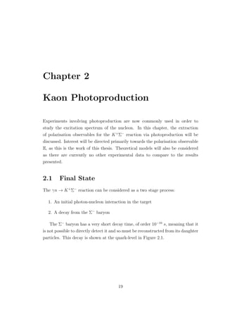
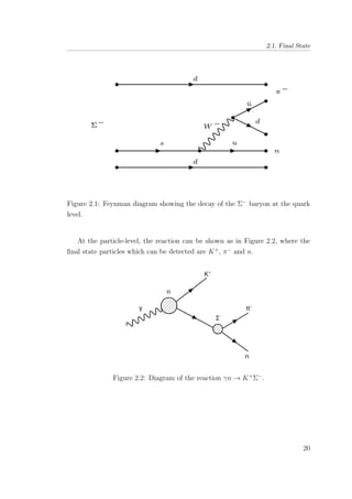
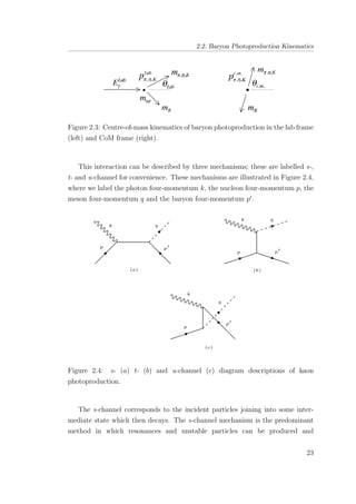
8.1 Diagram showing the kinematics for the γn → K+
Σ−
in the
centre-of mass frame. . . . . . . . . . . . . . . . . . . . . . . . 127
8.2 Energy spectrum of photons, after all event selections have
taken place. The binning is shown in red. . . . . . . . . . . . . 128
8.3 Centre-of-mass angular distribution for K+
. The binning is
shown in red. . . . . . . . . . . . . . . . . . . . . . . . . . . . . 129
8.4 E double-polarisation observable for empty target period A: all
energies (1.1-2.3 GeV ). . . . . . . . . . . . . . . . . . . . . . . 131
8.5 E double-polarisation observable for empty target period A: 1.1-
1.3 GeV (upper), 1.3-1.5 GeV (lower). . . . . . . . . . . . . . . 132
8.6 E double-polarisation observable for empty target period A: 1.5-
1.7 GeV (upper), 1.7-1.9 GeV (lower). . . . . . . . . . . . . . . 133
8.7 E double-polarisation observable for empty target period A: 1.9-
2.1 GeV (upper), 2.1-2.3 GeV (lower). . . . . . . . . . . . . . . 134
8.8 E double-polarisation observable for empty target period B: all
energies (1.1-1.3 GeV ). . . . . . . . . . . . . . . . . . . . . . . 135
8.9 E double-polarisation observable for empty target period B: 1.1-
1.3 GeV (upper), 1.3-1.5 GeV (lower). . . . . . . . . . . . . . . 136
8.10 E double-polarisation observable for empty target period B: 1.5-
1.7 GeV (upper), 1.7-1.9 GeV (lower). . . . . . . . . . . . . . . 137
8.11 E double-polarisation observable for empty target period B: 1.9-
2.1 GeV (upper), 2.1-2.3 GeV (lower). . . . . . . . . . . . . . . 138
8.12 K+
z vertex from the centre of CLAS, compared with scaled
empty target data. . . . . . . . . . . . . . . . . . . . . . . . . . 140
8.13 Photon energy (Eγ) vs photon polarisation. . . . . . . . . . . . 144
8.14 E double-polarisation observable in terms of the azimuthal angle
φ: all energies (1.1-2.3 GeV ). . . . . . . . . . . . . . . . . . . . 146
8.15 E double-polarisation observable in terms of the azimuthal angle
φ: 1.1-1.3 GeV (upper), 1.3-1.5 GeV (lower). . . . . . . . . . . 147
8.16 E double-polarisation observable in terms of the azimuthal angle
φ: 1.5-1.7 GeV (upper), 1.7-1.9 GeV (lower). . . . . . . . . . . 148
8.17 E double-polarisation observable in terms of the azimuthal angle
φ: 1.9-2.1 GeV (upper), 2.1-2.3 GeV (lower). . . . . . . . . . . 149
8.18 An event generator is used to compare the results of three
acceptances to a given true value of the double-polarisation
observable E (0.7). This shows the results for one trial. . . . . 152
xix](https://image.slidesharecdn.com/6d482e98-273b-437a-88cf-eb4faf084ce1-161109162450/85/thesis-20-320.jpg)
![1.1. Quantum Chromodynamics
in that they both describe interactions mediated by a massless spin − 1 boson
(gluons and photons respectively)2
.
Quarks exist in six flavours, along with their associated anti-particles:
• up (u & ¯u),
• down (d & ¯d),
• charm (c & ¯c),
• strange (s & ¯s),
• top (t & ¯t),
• bottom (b & ¯b).
These elementary particles, omitting the top quark, are able to form composite
particles, known as hadrons, using various combinations of two-quark (meson)
and three-quark (baryon) states, bound by gluons.
Gluons have no electric charge, like the photon, but instead couple to colour
charges, which should be conserved in all strong interactions3
. This gives a
flavour independence of the strong interaction, i.e. all flavours of quark must
have identical strong interactions as they may have the same values of colour
states. The crucial difference between QCD and QED is that gluons have the
ability to self-interact, as they themselves are bi-coloured, which is what defines
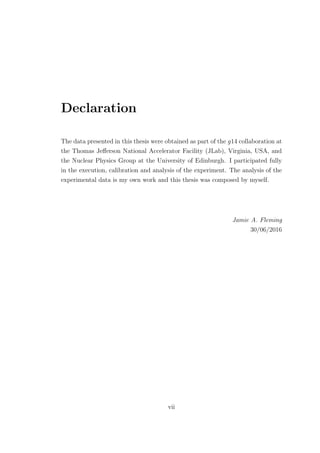
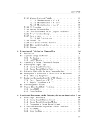
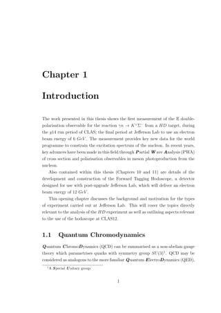
QCD as non-abelian. The self-interaction of gluons leads to the ability for three-
and four-gluon vertices, examples of which are illustrated in Figure 1.1. Gluonic
self-interaction leads to two other important properties; colour confinement and
asymptotic freedom.
Figure 1.1: Gluonic self-interaction.
2
More comprehensive formulations of QCD, in terms of interactions and mathematics, may
be found in [1] [2] [3].
3
Colours are defined as red (r), green (g) and blue (b); though not related to the physical
perception of colour but a tool to aid with the mathematical complications of QCD.
2](https://image.slidesharecdn.com/6d482e98-273b-437a-88cf-eb4faf084ce1-161109162450/85/thesis-29-320.jpg)
![1.1. Quantum Chromodynamics
Colour confinement can effectively be thought of as a condition that states
must be colour neutral. Moreover this leads to the requirement that there can be
no free quarks, as they have non-zero colour charge and must be contained in a
bound system with other quarks. Similarly for gluons, they may not be free but
can, in principle, be bound in states with other gluons, inside glueballs4
.
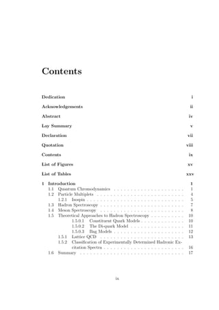
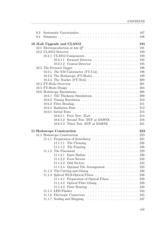
Asymptotic freedom means that the interaction becomes weaker at shorter
distances, and is echoed in the property that the coupling constant is not in fact
constant (often called a running coupling constant); the evolution of the running
coupling constant with energy is shown in Figure 1.2.
Figure 1.2: Summary of measurements of the strong coupling constant, αs(Q),
as a function of the energy scale, Q [4].
As the distance increases (> 1 fm) the higher order corrections of interactions
become more important. In this regime there are two main approaches:
1. Phenomenological models which include aspects expected from QCD but
4
The existence of the glueball remains to be established experimentally.
3](https://image.slidesharecdn.com/6d482e98-273b-437a-88cf-eb4faf084ce1-161109162450/85/thesis-30-320.jpg)
![1.2. Particle Multiplets
employing effective degrees of freedom. Such approaches are discussed
further in Section 1.5.0.1.
2. Obtaining solutions based on calculations using powerful computational
tools. Probably the most successful technique to date is that of Lattice
QCD (LQCD)5
. This approach is discussed further in Section 1.5.1.
It is also important to consider the effect of gluonic interactions within
hadrons. If we consider the proton, the constituent quark rest masses only
account for ∼ 1% of the total mass. This means that ∼ 99% of the mass
is dynamically generated from the non-perturbative interactions of quarks via
the exchange of gluons. These can self couple and interact with the vacuum
to produce quark-antiquark pairs. The net energy of all these processes then
produces the mass, from the equivalence between mass and energy (E = mc2
).
An artistic representation of this is shown in Figure 1.3. This demonstrates why
the internal dynamics of the proton and other hadrons are far from trivial.
Figure 1.3: A representation of quark and gluon interactions inside the nucleon
[7].
1.2 Particle Multiplets
After the discovery of the proton and neutron, it was postulated that they could
be considered as two states of the same particle, called the Nucleon [1]. At a
5
A more complete formalism of LQCD may be found in [5] [6].
4](https://image.slidesharecdn.com/6d482e98-273b-437a-88cf-eb4faf084ce1-161109162450/85/thesis-31-320.jpg)
![1.2. Particle Multiplets
cursory glance it can be seen that throughout the existing hadrons there are
sub-groups which seem to form families of particles with similar masses6
. For
example, the nucleons:
p(938) = uud,
n(940) = udd,
(1.1)
and the family of kaons:
K±
(494) = u¯s,
K0
(498) = d¯s.
(1.2)
These families are labelled Isospin Multiplets [1].
1.2.1 Isospin
Isospin, I, is a spin quantum number, which has its definition based in the
construction of these multiplets. Another quantum number can be introduced,
hypercharge Y :
Y = B + S + C + ˜B + T, (1.3)
where B, S, C, ˜B and T are the baryon number, strangeness, charm, beauty
and truth respectively. If we consider the members of a multiplet it can be seen
that these individual quantum numbers do not change, therefore neither does the
hypercharge. Here we see the third component of isospin, I3, defined in terms of
hypercharge and the electric charge, Q:
I3 = Q −
Y
2
. (1.4)
For the case of the nucleon, only the baryon number contributes to hyper-
charge (Y = 1), from Equation 1.4 this gives the values of I3 = +1/2 and
I3 = −1/2 for the proton and neutron respectively.
6
Other interesting properties which these families display are identical spin, parity, baryon
number, strangeness, charm and beauty.
5](https://image.slidesharecdn.com/6d482e98-273b-437a-88cf-eb4faf084ce1-161109162450/85/thesis-32-320.jpg)
![1.2. Particle Multiplets
The values of I3 for a multiplet run from ±I:
I3 = I, I − 1, ..., −I. (1.5)
If we extend our earlier example of nucleons and kaons, the quantum numbers
can be shown simply in Table 1.1 as:
Particle B Y Q I3 I
p(938) 1 1 1 1
2
1
2
n(940) 1 1 0 −1
2
1
2
K+
(494) 0 1 1 1
2
1
2
K0
(498) 0 1 0 −1
2
1
2
Table 1.1: Summary of nucleon and kaon properties.
We have only considered the variable of isospin, but these multiplets can be
extended in hypercharge space, giving rise to further families. This can be done
for mesons, as in Figure 1.4, and equivalently for baryons, as in Figure 1.5.
Figure 1.4: Meson nonet (B = 0) shown in terms of charge, Q, and strangeness,
S [8].
6](https://image.slidesharecdn.com/6d482e98-273b-437a-88cf-eb4faf084ce1-161109162450/85/thesis-33-320.jpg)
![1.3. Hadron Spectroscopy
Figure 1.5: Baryon octet (B = 1) shown in terms of charge, Q, and strangeness
S [9].
1.3 Hadron Spectroscopy
The internal structure of the nucleon and its interactions are key areas of interest
within the nuclear physics community. The excitation spectrum of the nucleon is
a very effective way to constrain nucleon dynamics; spectroscopy is the study of
these excited states. The excited states of the nucleon are resolvable in a limited
mass range, typically ∼ 1-2 GeV [10] [11]. As shown in Figure 1.2, the running
coupling constant is extremely large in this region, therefore perturbation theory
is no longer valid; this is shown explicitly in Figure 1.6 in terms of interaction
distance.
7](https://image.slidesharecdn.com/6d482e98-273b-437a-88cf-eb4faf084ce1-161109162450/85/thesis-34-320.jpg)
![1.4. Meson Spectroscopy
Figure 1.6: Evolution of the strong coupling constant, αs(Q), as a function of the
interaction distance [12].
Decays from resonances of excited nucleon states predominantly proceed via
the strong force. Intrinsically, strong processes occur over very short times,
leading to large peak widths, as expected from the uncertainty principle;
∆E∆t ≥
2
. (1.6)
Excited states with lifetimes of around 10−23
s, are seen with widths of
around 100 MeV . Resonances, however, are typically spaced much closer together
than this, leading to significant overlap of neighbouring peaks. This overlapping
structure makes a reliable extraction of the spectrum more challenging than in
the case of atomic or nuclear physics, when states can generally be well separated.
1.4 Meson Spectroscopy
The study of non-perturbative QCD is not of course limited to the nucleon studies
discussed above. Similar basic processes, in terms of hadronic structure and mass
generation mechanisms can also occur in mesons.
8](https://image.slidesharecdn.com/6d482e98-273b-437a-88cf-eb4faf084ce1-161109162450/85/thesis-35-320.jpg)
![1.4. Meson Spectroscopy
Central to the aim of the upgraded JLab facility is to obtain a complete map
of the spectrum of meson states in the range 1-3 GeV . This would provide a
unique fingerprint to constrain our understanding of the confinement of mesons7
.
States in the low mass region of the meson spectrum are relatively well
experimentally characterised [15]. However, the spectrum of higher mass states is
established with much poorer confidence and accuracy. As well as mesons states
expected from simple constituent quark models, others are predicted outwith the
allowed quantum numbers for a simple q¯q system. These take the form of more
exotic states like tetraquarks (q¯qq¯q), hybrids (qqg) and glueballs (gg) [16] [17]
[18] [19]. The latter two occur due to excited gluonic degrees of freedom within
the meson system, allowing for the quantum numbers of the gluonic field itself
to contribute to the mesonic state. Early theoretical approaches used a flux-tube
model [20] [21] for these gluonic components but major recent developments in
theory have allowed predictions directly from QCD.
The lowest of the exotic states are predicted around 2 GeV , from LQCD
calculations [22] [23]. The lightest of these predicted states include 1−+
, 0+−
and
2+−
in terms of JPC
. The hybrid and glueball mass range is thought to be around
1.4-3.0 GeV ; accessible with the 12 GeV beam energy which will be available at
JLab12.
In photoproduction, the production rate of hybrid mesons is thought to be
comparable to normal meson production rates and CLAS12 aims to exploit this
fact.
There is some weak and disputed evidence for a few of the predicted states [24]
[25] but new measurements and analyses are required to establish their existence
and properties. Also for a full confirmation of any of these states they must, of
course, be seen in more than one decay mode.
7
Other goals of the upgraded JLab include, better establishing the internal dynamics of the
nucleon, Generalised Parton Distributions (GPDs) and eventually achieving a 3D image of
the nucleon, by mapping out the momentum and spatial location of its constituents [11] [13]
[14].
9](https://image.slidesharecdn.com/6d482e98-273b-437a-88cf-eb4faf084ce1-161109162450/85/thesis-36-320.jpg)
![1.5. Theoretical Approaches to Hadron Spectroscopy
1.5 Theoretical Approaches to Hadron Spec-
troscopy
There exist many theoretical approaches to model hadrons and predict their
excited states. These methods either start from the underlying QCD Lagrangian
or attempt to incorporate various properties of QCD such as colour confinement
and asymptotic freedom in phenomenological degrees of freedom [26].
1.5.0.1 Constituent Quark Models
These phenomenological models treat the nucleon as a bound state of constituent
quarks, each of which are assigned one third of the nucleon mass [27]. These
constituent quarks are then bound with a quark-quark interaction which is based
on the one gluon exchange potential from QCD. The constituent quarks can be
thought of as a bare valence quark, as seen in QCD, which has been dressed in a
cloud of low-momenta virtual gluons, resulting in an effective mass mq = 1
3
mN .
These models have some success in predicting the spectra of experimentally
observed excited states. These models tend to predict many more states than
those currently observed. It is not currently established if this reflects a deficiency
in the theory or insensitivity in current experimental measurements. It should be
remarked however that a similar quantity of excited states have been predicted
from recent LQCD calculations, Section 1.5.1.
Figure 1.7 indicates states predicted by the constituent quark model and
highlights their experimental standing. In this plot the heavy uniform-width bars
show the predicted masses of states with well established counterparts from PWA,
light bars those of states which are weakly established or missing. The length
of the thin white bar gives the prediction for each states γN decay amplitude,
thin grey bar for its πN decay amplitude, and thin black bar for its KΣ decay
amplitude.
10](https://image.slidesharecdn.com/6d482e98-273b-437a-88cf-eb4faf084ce1-161109162450/85/thesis-37-320.jpg)
![1.5. Theoretical Approaches to Hadron Spectroscopy
Figure 1.7: Mass predictions, γN, πN, and KΣ decay amplitude predictions for
nucleon resonances up to 2200 MeV [28].
1.5.0.2 The Di-quark Model
This model considers the nucleon as a pair of quarks which are strongly correlated
and a third valence quark, reducing the number of degrees of freedom in the
system [29]. A simple illustration of this is given in Figure 1.8. The reduced
number of degrees of freedom results in fewer excited states than the qqq
constituent quark models.
Figure 1.8: Representation of the di-quark model inside the nucleon [30].
11](https://image.slidesharecdn.com/6d482e98-273b-437a-88cf-eb4faf084ce1-161109162450/85/thesis-38-320.jpg)
![1.5. Theoretical Approaches to Hadron Spectroscopy
This model has also had some success in predicting low energy resonances
[31], but results from LQCD [32] [33] seem to suggest that di-quarks do not
form inside the nucleon. The existence or non-existence of di-quarks is still an
unresolved question in the field.
1.5.0.3 Bag Models
Bag models attempt to explicitly model the colour confinement of quarks within
the hadron [34]. The model begins with some finite spherical potential, set at a
fixed radius, labelled the bag. Quarks are placed inside this potential, in which
they are seen as massless. The boundary conditions of the bag are set-up such
that the quarks are confined by a bag and out-with this volume they have infinite
mass. Perturbative QCD can then be used within these boundary conditions.
Variants on this model have also been developed, such as the MIT Bag Model
[18], the Cloudy Bag Model [35] and the SLAC Bag Model [36].
Bag models have had some success in predicting the masses of particles, shown
in Figure 1.9.
12](https://image.slidesharecdn.com/6d482e98-273b-437a-88cf-eb4faf084ce1-161109162450/85/thesis-39-320.jpg)
![1.5. Theoretical Approaches to Hadron Spectroscopy
Figure 1.9: Light baryon and meson masses, predicted by the bag model. The
actual masses are given by dotted lines, while all other masses are predicted. The
masses of N, ∆, Ω and ω were used to determine the parameters [26].
1.5.1 Lattice QCD
Lattice QCD is formulated upon a grid, named the lattice, in space-time. Fields
are used to represent quarks which are located at points on the lattice; between
these lattice points gluon fields are used to link quark fields, this is simply
illustrated in Figure 1.10. Within this framework, QCD predictions can be
extracted taking the limit, in which the lattice spacing is reduced to zero. The
complexity of numerical calculations increases dramatically as the lattice spacing
is reduced.
13](https://image.slidesharecdn.com/6d482e98-273b-437a-88cf-eb4faf084ce1-161109162450/85/thesis-40-320.jpg)
![1.5. Theoretical Approaches to Hadron Spectroscopy
Figure 1.10: Simple interpretation of QCD calculated on a lattice [37].
A central challenge of hadronic physics is to establish whether LQCD can fully
explain phenomena at these large distances and low momenta, where realistic
analytical predictions from QCD are intractable. The lattice approach offers the
possibility to obtain predictions based on QCD using computational methods
without explicitly solving the QCD Lagrangian.
Interestingly LQCD predicts many bound quark states beyond the simple
nucleon and meson that are yet to be observed experimentally and gives an
indication of the expected masses. This includes hybrid mesons, in which the
usual two quark degrees of freedom are supplemented with other dynamics [38].
In hybrid mesons the gluonic field which is created in the confinement process
of the two quarks can become a degree of freedom in itself. The additional parity
and angular momentum quantum numbers are predicted to give rise to exotics,
which have combinations of spin, parity and C-parity which cannot be reached
from only two degrees of freedom. The search for these objects is a key physics
goal of the Forward Tagger [39], discussed in Chapter 10.
In recent years LQCD has progressed such that prediction of the excitation
spectrum of the nucleon can be made, this method has had much success
predicting the lowest mass hadrons to experimental values to within 1% [40].
Currently computational limits mean that these calculations cannot be carried
out at realistically light quark masses in the nucleon, although there is rapid
14](https://image.slidesharecdn.com/6d482e98-273b-437a-88cf-eb4faf084ce1-161109162450/85/thesis-41-320.jpg)
![1.5. Theoretical Approaches to Hadron Spectroscopy
progress towards this. Current state-of-the-art calculations are carried out at
quark masses equivalent to a pion mass of ∼ 400 MeV (∼ 260 MeV above the
PDG value). The calculations are extrapolated to realistic quark masses using
phenomenological (although QCD-guided) extrapolations.
The spectra of predicted meson states is shown in Figure 1.11. States corre-
sponding to the established mesons are predicted, along with many unobserved
or poorly established states. Lattice QCD also predicts a whole family of hybrid
mesons which are unobserved. Clearly QCD may be a much richer environment
than currently established.
Figure 1.11: The spectra of isoscalar mesons calculated by the JLab LQCD group
(mπ ∼ 396 MeV ) [41].
Predictions for the baryon spectra are shown in Figure 1.12. Many more
excited states than currently established are predicted by the models, mirroring
the excess of states predicted by the qqq constituent quark model. Also hybrid
baryon states are predicted, excited nucleon states which have large gluonic
components in their wavefunction. Unfortunately such states do not have exotic
quantum numbers but are predicted in a mass range where there is a paucity of
qqq states. Future experiments will search for these exotic objects.
15](https://image.slidesharecdn.com/6d482e98-273b-437a-88cf-eb4faf084ce1-161109162450/85/thesis-42-320.jpg)
![1.5. Theoretical Approaches to Hadron Spectroscopy
Figure 1.12: The spectra of baryons calculated by the JLab LQCD group (mπ ∼
396 MeV ), in units of the calculated Ω mass [42].
The results support the idea that there may be many excited nucleon states
that remain to be established experimentally. It is crucial to establish whether
this is due to a lack of sensitivity in the measurements or whether this is telling
us about something lacking in the underlying theory to describe non-perturbative
QCD.
1.5.2 Classification of Experimentally Determined Hadronic
Excitation Spectra
In identifying resonant states experimentally it is imperative to determine
quantum numbers, particle mass, branching ratios and widths to challenge
the theoretical models. The Particle Data Group (PDG) collects data for
experimentally observed states; using a star system to indicate the confidence
level of each determination, based on the consistency of sightings in different
analyses and the significance of the signals obtained. The different ratings are
defined below:
• **** Existence is certain, and properties are at least fairly well explored
• *** Existence is very likely but further confirmation of decay modes is
required
• ** Evidence of existence is only fair
16](https://image.slidesharecdn.com/6d482e98-273b-437a-88cf-eb4faf084ce1-161109162450/85/thesis-43-320.jpg)
![1.6. Summary
• * Evidence of existence is poor
Until around a decade ago, most data on resonances came from the study of
πN scattering experiments. Recently, photoproduction is being used as a powerful
experimental tool and has established five new resonances in recent years [43].
This new sensitivity has arisen from the quality of the photoproduction data and
differences in the relative coupling of the missing resonances to the πN and γN
channels. The cross sections of meson photoproduction from the proton are shown
in Figure 1.13, separated according to the different strong decay channels. It has
been predicted that some missing resonances may couple strongly to “strange”
photoproduction channels [28]; meaning that the channels KΛ and KΣ are of
specific interest.
Figure 1.13: Photoproduction cross section of γp (log scale), including the
magnitude of channels contributing to the total cross section [44].
1.6 Summary
Given the non-perturbative behavior of QCD at low energies, states must be
investigated through approximate solutions of QCD such as QCD-inspired models
17](https://image.slidesharecdn.com/6d482e98-273b-437a-88cf-eb4faf084ce1-161109162450/85/thesis-44-320.jpg)
![2.3. Reaction Amplitudes
σ =
4π
dσ
dΩ
dΩ. (2.9)
The differential cross section of a photoproduction reaction can be written in
terms of s and t, from Equation 2.8, in an amplitude, A, which is a function of
the outgoing momentum and the scattering angle:
dσ
dΩ
= A(s, cos θ)A(s, cos θ) ∼ |A(s, cos θ)|2
. (2.10)
Any function of θ can be written in terms of associated Legendre polynomials,
Φl(cos θ). The scattering amplitude can be written in terms of the Mandelstam
variable s and these polynomials:
A(s, cos θ) =
4
√
s
∞
l=0
(2l + 1)al(k)Φl(cos θ), (2.11)
where l is the relative orbital angular momentum between the target and the
scattered particle, and al(k) is defined as the lth
partial wave amplitude [45].
The scattering amplitudes can be decomposed into several of these partial wave
amplitudes, each denoting scattering in a particular angular momentum.
The photoproduction process can be described mathematically using the
scattering matrix, S. The matrix represents the probability of the transition
from the initial to final state. The method relates the initial and final states, in a
way which allows computation of probabilities related to the scattering process.
The initial photon and nucleon state is defined with an eigenstate i|; while the
final meson and baryon state is defined with the eigenstate |f , related by the
scattering matrix, S:
i|S|f . (2.12)
The scattering matrix can be described in terms of the particle four-momenta,
k, p, q and p , and the transition matrix, Tfi:
Sfi = δfi − i(2π)4
δ4
(k + p − q − p )Tfi. (2.13)
The first term here represents the possibility of no scattering, while the second
is the scattering term. The transition matrix is a type of stochastic matrix, where
25](https://image.slidesharecdn.com/6d482e98-273b-437a-88cf-eb4faf084ce1-161109162450/85/thesis-52-320.jpg)
![2.4. Polarisation Observables
the entries represent the probability of transitions between states.
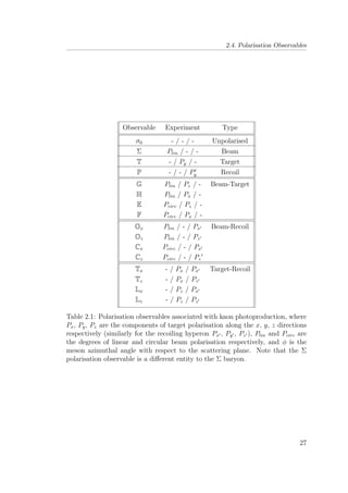
2.4 Polarisation Observables
In order to fully understand the photoproduction process and extract unambigu-
ous information on intermediate nucleon resonance contributions, it is important
to make measurements in addition to the unpolarised differential cross section.
These additional observables are extracted by measuring the dependencies of the
differential cross section to the known polarisation of the particles involved in the
reaction. Specifically for the case of strangeness photoproduction these consist
of:
1. Incident photon,
2. Target nucleon,
3. Recoiling hyperon.
Scattering amplitudes in kaon photoproduction are constructed using Chew
Goldberger Low N ambu (CGLN) amplitudes [46]. Four of these complex
amplitudes are necessary to describe the degrees of freedom of the incident photon
and nucleon system. Taking bilinear combinations of these amplitudes allow for
16 independent polarisation observables to be constructed [47], shown in Table
2.1.
The single-polarisation observables arise when only the polarisation of one
of the beam, target or recoil is measured in the reaction. Double-polarisation
observables are split into three groups: Beam-Target, Beam-Recoil and Target-
Recoil. Within these three groups multiple measurements must be made to
identify all possible observables. For example, for the Beam-Target observables
measurements must be made using all combinations of linearly and circularly
polarised beam incident on a transversely and longitudinally polarised target.
Since these observables are derived from four complex amplitudes, they are
not independent. This means that all observables for a photoproduction process
can be known by only measuring a sub-set of these 16. Relations between these
observables are shown as follows [48]:
26](https://image.slidesharecdn.com/6d482e98-273b-437a-88cf-eb4faf084ce1-161109162450/85/thesis-53-320.jpg)
![2.5. Isolating a Polarisation Observable
E2
+ F2
+ G2
+ H2
= 1 + P2
− Σ2
− T2
,
FG − EH = P − ΣT,
T2
x + T2
z + L2
x + L2
z = 1 + Σ2
− P2
− T2
,
Tx Lz − Tz Lx = Σ − PT,
C2
x + C2
z + O2
x + O2
z = 1 + T2
− P2
− Σ2
,
C2
z O2
x − C2
x O2
z = T − PΣ.
(2.14)
Beyond determining a single polarisation observable, a goal of these meson
photoproduction experiments is to perform a full set of measurements on a
channel in order to unambiguously constrain the amplitude. Many of these
experiments are non-trivial so it is beneficial that all 16 polarisation observables
need-not be measured in order to fully define the amplitude.
Measurement of the single-polarisation observables (Σ, T, P) must be made
[47], as well as taking a selected number of double-polarisation observables. The
exact number and nature of these double-polarisation observables was debated
and disagreed upon. This was finally settled by Chiang and Tabakin [49], who
showed that four appropriately chosen double-polarisation observables along with
the cross section and single-polarisation observables are enough to fully determine
the amplitude unambiguously.
2.5 Isolating a Polarisation Observable
The differential cross section is classified into three expressions dependent on
the type of double-polarisation experiment being conducted. Considering an
experiment with polarised photons incident on a polarised target:
dσ
dΩ
=
dσ
dΩ 0
[1 − PlinΣ cos(2φ)
+ Px(−PlinH sin(2φ) + PcircF)
+ Py(T − PlinP cos(2φ))
+ Pz(PlinG sin(2φ) − PcircE)].
(2.15)
28](https://image.slidesharecdn.com/6d482e98-273b-437a-88cf-eb4faf084ce1-161109162450/85/thesis-55-320.jpg)
![2.6. Theoretical Models for Meson Photoproduction
Considering an experiment with Beam-Recoil measurements:
dσ
dΩ
=
dσ
dΩ 0
[1 − PlinΣ cos(2φ)
+ Px (−PlinOx sin(2φ) − PcircCx )
+ Py (P − PlinT cos(2φ))
+ Pz (−PlinOz sin(2φ) − PcircCz )].
(2.16)
Finally, considering an experiment with Target-Recoil measurements:
dσ
dΩ
=
dσ
dΩ 0
[1 + PyT + Py P
+ Px (PxTx − PzLx )
+ Py PyΣ
+ Pz (PxTz + PzLz )].
(2.17)
In this thesis, the observable of interest is the Beam-Target observable E.
From Table 2.1, in order to study the observable E, a circularly polarised photon
beam and a longitudinally polarised target must be used. Other components
of the target polarisation are therefore zero, Px = Py = 0, while there is no
contribution from a linearly polarised photon beam, Plin = 0. We simplify our
expression for the Beam-Target differential cross section, Equation 2.15, using
these conditions:
dσ
dΩ
=
dσ
dΩ 0
[1 − PzPcircE]. (2.18)
2.6 Theoretical Models for Meson Photopro-
duction
Information on the nucleon resonance spectrum is extracted by fitting a model
to experimental data and fitting parameters in the model to extract the masses,
29](https://image.slidesharecdn.com/6d482e98-273b-437a-88cf-eb4faf084ce1-161109162450/85/thesis-56-320.jpg)
![2.6. Theoretical Models for Meson Photoproduction
widths and quantum numbers of the contributing resonances [50]. As this fitting
separates the contributions from different angular momenta (partial waves) it is
often referred to as a Partial W ave Analysis (PWA) [38].
These models consider the processes as being comprised of a resonant and
background component. These components are parametrised and extracted
from the experimental data through fitting. As with many models, the more
experimental data which is available, the more constraints can be placed upon
the reaction channel to provide more accurate and less ambiguous results.
If we consider a generic reaction where we have a photon-nucleon interaction,
a, with some intermediate resonance state, c, which finally ends in a meson-
nucleon system, b, the Hamiltonian can be written as:
H = H0 + V, (2.19)
where the first term is the free Hamiltonian, H0, and the second is the interaction
term, V. As is a common feature of reaction models, this interaction term is split
into a resonant component, VR, and a background component, VB:
V = VR(E) + VB, (2.20)
where the resonant component is a function of the total energy, E.
The probability of the process to occur is governed by a transition matrix,
Tba, which can be similarly reduced into components:
Tba(E) = TR
ba(E) + TB
ba. (2.21)
The resonant component of this transition matrix can be expanded by
summing over all possible paths in the process a → c → b, and introducing
a propagator of state c, gc;
Tba(E) =
c
Vbagc(E)Tbc(E) + Vba. (2.22)
2.6.1 Isobar Models
Isobar models attempt to use an effective Lagrangian to simulate the properties
of interactions. They do this by evaluating tree-level Feynman diagrams for the
30](https://image.slidesharecdn.com/6d482e98-273b-437a-88cf-eb4faf084ce1-161109162450/85/thesis-57-320.jpg)
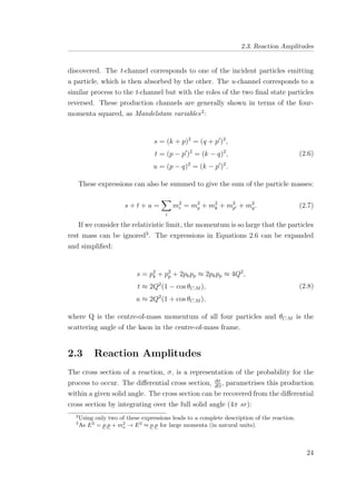
![2.6. Theoretical Models for Meson Photoproduction
resonant and non-resonant exchange of mesons and baryons. By considering
the possible exchanges which take place in s-, t- and u-channel reactions, excited
states can be identified. This tree-level method is useful to simplify the interaction
to first order, but neglects to take into account effects such as interactions in the
final state or coupled-channel effects.
The isobar model we will consider in this thesis is the KaonMAID model [51]4
.
The model considers low-order diagrams for the interaction, which are then split
into resonant and non-resonant terms (Born terms). The s-channel mechanism
represents the resonant contributions, while the t- and u-channel mechanisms
represent the background contribution.
These isobar models have seen much use in the energy region under 2 GeV
due to the smaller importance of higher order diagrams and Born terms at lower
energies. The models attempt to produce theoretical predictions of polarisation
observables using various combinations of resonances. This allows for comparison
between data and prediction in order to infer the presence or absence of a
resonance. This is not a trivial procedure as many partial waves can be present
and interfere strongly.
2.6.2 Coupled-Channel Analysis
Coupled-Channel (CC) analysis is an attempt to improve the accuracy of the
isobar model to include final state particle interactions, as well as intermediate
states such as πN5
. These processes can be described as production of a non-
resonant state which rescatters from the nucleon in order to produce a resonance.
Coupled-channel analysis also hopes to reduce the ambiguity of resonance
combinations used to fit data [52]. As it is possible for more than one combination
of resonances to fit the data well, this disambiguous nature can be removed by
considering multiple observables on multiple final states. This analysis method
allows more constraints to be added to the channel which acts as a filter to remove
resonances which do not contribute to the final state.
The model we wish to consider in this thesis is the Bonn-Gatchina (BoGa)6
.
4
Maintained and developed by the Institut f¨ur Kernphysik, Universit¨at Mainz, Germany.
5
Amplitudes of γN → πN process is thought to play a considerable effect in the overall
process γN → πN → KY , where Y is a final state hyperon.
6
Maintained and developed by the Helmholtz-Institut f¨ur Strahlen- und Kernphysik,
Universit¨at Bonn, Germany; and Kurchatov Institute, Petersburg N uclear Physics I nstitute
31](https://image.slidesharecdn.com/6d482e98-273b-437a-88cf-eb4faf084ce1-161109162450/85/thesis-58-320.jpg)
![2.7. Summary
This is a coupled-channel model which aims to consider multiple decay
channels at once, with angular and energy dependencies of different observables
are analysed simultaneously [53]. This provides stable fits for partial waves with
high spin and provides a smooth behaviour in energy.
Two particle final states, such as πN, ηN, KΛ, KΣ, ωN and K∗
Λ are
fitted with the χ2
method. At fixed energies, the unpolarised cross section of
pseudoscalar mesons is characterised by the differential cross section only. For
vector mesons however, the unpolarised cross section is characterised by the
differential cross section and three spin density matrix elements.
2.7 Summary
Experiments utilising both polarised beams and targets are crucial in gathering
data in order to characterise photoproduction scattering amplitudes. Reaction
models such as KaonMAID and Bonn-Gatchina can be fitted to experimental
data and used to extract properties of nucleon resonances contributing to the
reaction.
An outline of the process is shown in Figure 2.5, showing the relations between
the experiment, reaction model theory and QCD.
(PNPI), Gatchina, Russia.
32](https://image.slidesharecdn.com/6d482e98-273b-437a-88cf-eb4faf084ce1-161109162450/85/thesis-59-320.jpg)
![2.7. Summary
Figure 2.5: Process for nucleon structure calculation and experimentation [54].
33](https://image.slidesharecdn.com/6d482e98-273b-437a-88cf-eb4faf084ce1-161109162450/85/thesis-60-320.jpg)
![Chapter 3
Previous Experimental Data
In this chapter, key experimental data from the K+
Σ−
channel are discussed.
Since there are no previous measurements for the E double-polarisation ob-
servable, these measurements focus on differential cross sections and beam-
asymmetries.
3.1 Current Experimental Knowledge
Polarisation observable experiments from strangeness channels from neutron
targets are relatively few: this is particularly true for the reaction γn → K+
Σ−
.
Experiments were conducted at Cornell in the late 1950s, followed by experiments
at LEPS and Jefferson Lab in the mid-2000s.
3.1.1 Kaon Photoproduction at Cornell
The experiment which took place at Cornell in the 1950s aimed to measure the
differential cross section of the γn → K+
Σ−
reaction [55]. This used both liquid
hydrogen and liquid deuterium target with kaon momenta of 0.405 and 0.455
GeV , and a bremsstrahlung beam of peak energy 1.170 GeV .
They wished to consider the total K+
photoproduction cross section from
three reaction channels:
34](https://image.slidesharecdn.com/6d482e98-273b-437a-88cf-eb4faf084ce1-161109162450/85/thesis-61-320.jpg)
![3.1. Current Experimental Knowledge
k θCM γp → K+
Σ0 γn→K+Σ−
γp→K+Σ0
(MeV ) (◦
) (10−31
cm2
/sr)
1122 82 0.6 ± 0.1 1.6 ± 0.7
1146 75 1.1 ± 0.2 0.8 ± 0.6
Table 3.1: Data points and associated errors obtained from cross section
measurements at Cornell [55].
γp → K+
Λ,
γp → K+
Σ0
,
γn → K+
Σ−
.
(3.1)
The cross sections from the proton had already been measured at Cornell
in 1959/60 respectively [56] [57]. From the total kaon yield and the previous
measurements at Cornell, it was possible to estimate the cross section for the
K+
Σ−
reaction. Only two data points were obtained from this analysis, with
error bars of order ∼ 50%, these are shown in Table 3.1.
3.1.2 Kaon Photoproduction at LEPS
The experiment which took place at the Laser Electron Photon beam-line at
SPring−8 (LEPS) in the 2000s, aimed to measure differential cross sections and
photon-beam asymmetries for the γn → K+
Σ−
and γp → K+
Σ0
reactions [58].
This used linearly polarised photons on liquid hydrogen and deuterium targets.
The photon beam was of energy 1.5 - 2.4 GeV with a high polarisation (typically
∼ 90% at 2.4 GeV ) , with kaons measured at 0.6 < cos θK+
CM < 1.0.
Differential cross sections for K+
Σ−
and K+
Σ0
in four angular bins were
obtained, shown in Figure 3.1. They found the cross sections of both channels
were comparable at higher energies. The theoretical models tended to agree well
with the K+
Σ0
data but overestimate the K+
Σ−
data at higher energies.
35](https://image.slidesharecdn.com/6d482e98-273b-437a-88cf-eb4faf084ce1-161109162450/85/thesis-62-320.jpg)
![3.1. Current Experimental Knowledge
Figure 3.1: Differential cross sections for γn → K+
Σ−
(circles) and γp → K+
Σ0
(squares). Only statistical errors are shown. The solid and dashed curves are
the Regge model [59] calculations for the K+
Σ−
and K+
Σ0
, respectively. The
dotted curve is the KaonMAID model calculations for the K+
Σ−
[58].
Measurements for the photon-beam asymmetry were also taken, Figure 3.2.
These indicated the asymmetries of K+
Σ−
were typically larger than for the
K+
Σ0
channel. Another key feature was the increase in asymmetry for K+
Σ0
with the centre-of-mass energy, whereas K+
Σ−
shows minimal dependence above
2 GeV . The Regge model agrees well with the K+
Σ−
channel but overestimates
the K+
Σ0
channel.
36](https://image.slidesharecdn.com/6d482e98-273b-437a-88cf-eb4faf084ce1-161109162450/85/thesis-63-320.jpg)
![3.1. Current Experimental Knowledge
Figure 3.2: Photon-beam asymmetries for γn → K+
Σ−
(circles) and γp → K+
Σ0
(squares). The solid and dashed curves are the Regge model calculations for the
K+
Σ−
and K+
Σ0
, respectively [58].
3.1.3 Kaon Photoproduction at Jefferson Lab
The ‘g10’ experiment which took place at Jefferson Lab in the 2000s, measured
the differential cross section of the γD → K+
Σ−
(ps) reaction using the Hall-B
CLAS detector [60]. The experiment used a bremsstrahlung photon beam with
energies 0.8 - 1.6 GeV on a liquid deuterium target, measuring kaons with centre-
of-mass angles between 10 - 140◦
. The data are shown, along with the data from
LEPS in Figure 3.3.
37](https://image.slidesharecdn.com/6d482e98-273b-437a-88cf-eb4faf084ce1-161109162450/85/thesis-64-320.jpg)
![3.1. Current Experimental Knowledge
Figure 3.3: Differential cross sections of the reaction γD → K+
Σ−
(ps) obtained
by CLAS (full circles). The error bars represent the total (statistical plus
systematic) uncertainty. LEPS data (empty triangles) and a Regge-3 model
prediction (solid curve) are also shown. Notice the logarithmic scale for high
energy plots [60].
This was the first high precision measurement of the Σ−
photoproduction
from the neutron over a broad range of kaon angle and photon energies. At
photon energies of ∼ 1.8 GeV a predominant peak in the forward direction begins
to form as the photon energy increases. This peak is attributed to increased
contributions from t-channel mechanisms, whereas at lower energies s-channel
mechanisms dominate. At energies above ∼ 2.1 GeV show possible indications
of a backwards peak beginning to form, thought to be coming from the presence
of u-channel mechanisms.
38](https://image.slidesharecdn.com/6d482e98-273b-437a-88cf-eb4faf084ce1-161109162450/85/thesis-65-320.jpg)
![Chapter 4
Experimental Apparatus
In this chapter, the main features of the Jefferson Lab facility and the
experimental set-up in Hall B are discussed.
4.1 Experimental Overview
The data used in this analysis for this thesis were taken during the g14 (HDice)
run period at the Thomas Jefferson N ational Accelerator Facility (TJNAF -
JLab), in Virginia, USA. The dates during which this experiment was carried
out were from November 2011 until May 2012. This timeframe corresponds
to the experimental proposal “N∗
Resonances in Pseudoscalar-Meson Photo-
Production from Polarized Neutrons in
−→
H.
−→
D and a Complete Determination
of the γn → K0
Λ Amplitude” (E06-101) [61]. This experiment used linearly and
circularly polarised photon beams on a frozen spin HD target in order to extract
polarisation observables.
4.2 Jefferson Lab
JLab consists of four experimental halls: A, B and C have been long-standing
constructions used in many iterations of JLab physics research; Hall D is a newly
built experimental facility.
Feeding these experimental halls is the Continuous Electron Beam Accelerator
Facility (CEBAF). An aerial view of the facility is shown in Figure 4.1. CEBAF
allows for a 6 GeV electron beam to be simultaneously delivered to up to three
39](https://image.slidesharecdn.com/6d482e98-273b-437a-88cf-eb4faf084ce1-161109162450/85/thesis-66-320.jpg)
![4.3. CEBAF
experimental halls, meaning that each hall may pursue its own experimental
program independently of the others.
Figure 4.1: Aerial view of the JLab facility, highlighting the CEBAF accelerator
and experimental halls [62].
Prior to May 2012, the facility and its detectors were designed to perform
experiments with a maximum beam energy of 6 GeV . The g14 experiment was
the final incarnation and this date marked the end of what was generally referred
to as JLAB6. Subsequently an upgrade began across the entire facility to enable
the production and receipt of a 12 GeV electron beam - JLAB12.
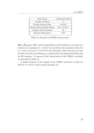
4.3 CEBAF
The CEBAF accelerator consists of two anti-parallel superconducting LIN ear
ACcelerators (LINACs) connected using recirculation arcs to form a “racetrack”
accelerator with a total length of 1.4 km. The main components of the CEBAF
accelerator are shown in Figure 4.2.
40](https://image.slidesharecdn.com/6d482e98-273b-437a-88cf-eb4faf084ce1-161109162450/85/thesis-67-320.jpg)
![4.3. CEBAF
Figure 4.2: Schematic of CEBAF at Jefferson Lab, including the experimental
halls [63].
An aggregate of nine arcs are used to recirculate beam-bunches allowing them
to be further accelerated with each pass through the LINAC sections, gaining
energies of up to 6 GeV . Multiple recirculation arcs are needed in order to
accept electrons after each new pass through the LINAC sections. The set of four
recirculation arcs in the east also contain an RF separator [64], which allows the
beam to be extracted and sent to individual experimental halls.
The electrons injected into the CEBAF accelerator are initially produced using
a 780 nm laser incident on a Gallium Arsenide (GaAs) photocathode. After initial
acceleration by an anode potential, these electrons are then accelerated to 67
MeV in the injector1
and separated into 2.0005 ns beam buckets, which are then
injected into the CEBAF accelerator. The electrons circle the racetrack up to five
times, gaining up to 0.6 GeV in each LINAC. The LINACs use superconducting
1
The injector consists of three pulsed lasers, one which supplies each hall, striking the
photocathode at a rate of 499 MHz leads to the characteristic ∼ 2 ns beam bucket structure
of CEBAF. The use of three separate lasers also allows each beam to have independent current
and polarisations.
41](https://image.slidesharecdn.com/6d482e98-273b-437a-88cf-eb4faf084ce1-161109162450/85/thesis-68-320.jpg)
![4.4. Experimental Halls
Figure 4.3: Schematic of CEBAF at Jefferson Lab, showing additions for the
upgrade to the beam-line, including the placement of the new Hall D [65].
4.4 Experimental Halls
Halls A, B, C and D are each equipped with bespoke detector systems. Hall D,
is the fourth experimental hall to be constructed off the beam-line of CEBAF;
this was recently completed in the quadrant off the northern LINAC, shown in
Figure 4.3.
The physics explored at JLab centres on exploring the nature of the nucleon.
Each hall uses its experimental set-up to probe various properties:
• Hall A [66]:
– Largest experimental hall containing two high-resolution spectrome-
ters.
– Experiments study: nucleon form factors, strange-quark structure of
the proton, and nucleon spin structure.
43](https://image.slidesharecdn.com/6d482e98-273b-437a-88cf-eb4faf084ce1-161109162450/85/thesis-70-320.jpg)
![4.5. Hall B
• Hall B [67]:
– Smallest experimental hall, containing CLAS; a spectrometer with a
nearly full angular range (∼ 4π) based around a toroidal magnetic
field.
– Experiments study: excited states of the nucleon, 3D imaging of the
nucleon’s quark structure and nucleon-nucleon correlations in nuclei,
exotic and hybrid mesons.
• Hall C [68]:
– Contains a high momentum spectrometer, using unique set-ups for
each experiment.
– Experiments study; weak interaction of the proton, transitions from
hadrons to quarks and strange nuclei.
• Hall D [69]:
– Contains a hermetic detector based around a solenoid magnet, de-
signed for use with JLAB12.
– Experiments will study: exotic and hybrid mesons.
During 6 GeV operation, Halls A and C received much greater beam currents
than that supplied to Hall B; typical beam currents are 100 µA and 10 nA
respectively. This factor of 104
difference is necessary due to the luminosity
restrictions of the Hall B detectors, which were not designed for high-flux
measurements. The fact that CEBAF is able to deliver beam currents with such
divergent beams simultaneously is a major achievement of the accelerator.
The g14 experiment was conducted in Hall B, therefore the remainder of the
chapter will be dedicated to exploring the Hall B experimental set-up.
4.5 Hall B
Hall B is the smallest experimental hall at Jefferson Lab and within it, the
CEBAF Large Acceptance Spectrometer (CLAS) is situated. A schematic view
of Hall B is shown in Figure 4.4. Although electron beam is delivered to the halls;
44](https://image.slidesharecdn.com/6d482e98-273b-437a-88cf-eb4faf084ce1-161109162450/85/thesis-71-320.jpg)
![4.5. Hall B
for some experiments, such as g14, it is desirable to use polarised photons on a
target. This is achieved in Hall B using a some kind of medium (a radiator) in
order to produce bremsstrahlung photons.
Figure 4.4: Diagram showing the scale of CLAS in Hall B at Jefferson Lab [63].
4.5.1 The Bremsstrahlung Process
The photon beam produced for use with CLAS uses electrons incident upon a
radiator, which decelerates the electrons while they interact with the electromag-
netic field of nuclei. Due to conservation of energy, the decelerated electrons must
emit the energy it has lost, which takes the form of a photon. The bremsstrahlung
method allows for the production of photons with energies in the range of 20−95%
of the incident electron beam energy [70]. A simple representation of this process
is shown in Figure 4.5.
45](https://image.slidesharecdn.com/6d482e98-273b-437a-88cf-eb4faf084ce1-161109162450/85/thesis-72-320.jpg)
![4.5. Hall B
Figure 4.5: Simple illustration of bremsstrahlung radiation [71].
Bremsstrahlung is kinematically possible if only a small amount of momentum
is transferred to the radiator nucleus, −→q ∼ 0. This is actually the typical method
of energy loss for electrons in material, and the nucleus recoil energy can usually
be neglected.
4.5.2 Bremsstrahlung Photon Tagging
Hall B has the ability to use CEBAF’s electron beam to create a photon beam for
use with certain targets [70]. In the case of the g14 experiment, both linearly and
circularly polarised photon beams were required for use on a HD target. Photons
were “tagged”, event-by-event, by the tagging spectrometer, which consists of a
large dipole magnet and a focal plane hodoscope. The dipole magnet bends
the electrons from the beam-line towards the timing and energy counters in the
hodoscope. A schematic of the tagging spectrometer is shown in Figure 4.6.
46](https://image.slidesharecdn.com/6d482e98-273b-437a-88cf-eb4faf084ce1-161109162450/85/thesis-73-320.jpg)
![4.5. Hall B
Figure 4.6: Schematic of the coherent bremsstrahlung facility in Hall B [70].
The electron and photon beams emerge from the radiator approximately
parallel to the incident electron beam, and are produced with an angular
distribution as follows:
θc =
1
γ
=
mc2
Ee−
, (4.1)
where m is the electron rest mass. The electron scattering angle is a function of
the photon production angle, energy and the electron energy:
θe− = θc
Eγ
Ee−
=
mc2
Eγ
Ee− Ee−
. (4.2)
For typical JLab energies, to a first approximation, the photons and electrons
are parallel. The photon and electron beams are then separated using the dipole
tagger magnet. The electrons are bent downwards while the photons continue
down the beam-line to interact with the target.
The tagging hodoscope consists of two separate layers of scintillator arrays.
The upper plane of scintillation counters (E-counters) are used to measure the
energy of the bent electrons after the bremsstrahlung emission, Ee− . When
combining this measurement with knowledge of the initial electron beam energy,
Ee− , a simple calculation of the produced photon energy, Eγ can be made:
47](https://image.slidesharecdn.com/6d482e98-273b-437a-88cf-eb4faf084ce1-161109162450/85/thesis-74-320.jpg)
![4.5. Hall B
Eγ = Ee− − Ee− . (4.3)
The E-counters allow for energy resolution of up to 0.0013 × Ee− .
The lower plane of scintillation counters (T-counters) are used to measure the
timing of the photon, with a resolution of ∼ 300 ps. This timing measurement
allows the electron to be correlated with its bunch and can be used to calculate
the photon time at the target. A full description of the tagging hodoscope can
be found within [70].
4.5.3 Beam Polarisation
Hall B is able to run using both linearly and circularly polarised photon beams.
These running modes require special conditions in the bremsstrahlung process.
4.5.3.1 Linear Polarisation
In Hall B, linearly polarised photons are generated from an unpolarised electron
beam using the coherent bremsstrahlung technique [72] [73]. This results in two
contributions to the photon spectrum; one from polarised (coherent) and another
from unpolarised (incoherent) bremsstrahlung photons2
.
In Hall B, the electron beam is scattered from a diamond radiator, of thickness
50 µm, in order to produce a linearly polarised photon beam from coherent
bremsstrahlung. Further information on the diamond radiator and linearly
polarised beam can be found in [74].
4.5.3.2 Circular Polarisation
To produced circularly polarised photons, it is required that a longitudinally
polarised electron beam be used. Foil was used as a radiator in this case, with
two main properties considered before a material was chosen:
1. Minimise the number of electron interactions
2. Maximise the probability of interaction
2
This is true for both linearly and circularly polarised periods.
48](https://image.slidesharecdn.com/6d482e98-273b-437a-88cf-eb4faf084ce1-161109162450/85/thesis-75-320.jpg)
![4.5. Hall B
This first property leads to the realisation that very thin foils must be used to
ensure that statistically one electron produces one photon. The second property,
when coupled with the information that the cross section for bremsstrahlung
emission is proportional to Z2
[75]3
, leads to the realisation that high-Z materials
should be used. The chosen material was a foil of gold (Z = 79) with thickness
10−4
radiation lengths.
The degree of circular polarisation obtained from this method is dependent on
the ratio of the photon energy, Eγ, and the incident electron energy, Ee− , often
labelled x for convenience (x = Eγ/Ee− ):
Pcirc =
4x − x2
4 − 4x + 3x2
Pe− , (4.4)
where Pcirc and Pe− are the photon circular and electron helicity polarisations
respectively. The distribution of the transfer of polarisation is shown in Figure
4.7.
Figure 4.7: Degree of circular polarisation as a function of the ratio of beam
energies, Eγ/Ee− [76].
3
Z denotes the atomic number of the material, which indicates the number of protons in the
nucleus.
49](https://image.slidesharecdn.com/6d482e98-273b-437a-88cf-eb4faf084ce1-161109162450/85/thesis-76-320.jpg)
![4.5. Hall B
4.5.4 CLAS Detector
The CEBAF Large Acceptance Spectrometer (CLAS) is housed in Hall B of the
Jefferson Lab facility. CLAS is a combination of many different types of particle
detector, giving almost complete angular coverage (∼ 4π) [67]. CLAS is built
around six superconducting coils, which produce a toroidal magnetic field, giving
a field-free region at the centre for use with polarised targets. These coils split
CLAS into six azimuthal regions going outward, which are defined as sectors.
The design is focused keenly on accurate detection of charged particles with good
momentum resolution. A diagram of CLAS and its associated sub-detectors is
shown in Figure 4.8.
Figure 4.8: The CLAS detector, including drift chambers, Cherenkov counters,
electromagnetic calorimeters, and time-of-flight detectors [77].
When a photon beam is used in Hall B, these photons interact with a target at
the centre of CLAS, causing a cascade of reaction products. These particles travel
outwards from the centre of CLAS passing through the multiple detector layers.
Particles firstly travel through the STart counter (ST), giving the start time of
50](https://image.slidesharecdn.com/6d482e98-273b-437a-88cf-eb4faf084ce1-161109162450/85/thesis-77-320.jpg)
![4.5. Hall B
the event. Particles then pass through the Drift Chambers (DC) which, using the
toroidal field, measures the bending of particles in order to calculate their velocity
and therefore momenta. They then pass through the time-of-flight Scintillation
Counters, giving the particle flight time from the target. The final layers are
focussed on forward particle detection; the penultimate being the Cherenkov
Counters and the final being the Electromagnetic Calorimeter 4
. These final
layers are used in electron beam experiments where negative pion and electrons
must be separated. Further information on the CC and EC can be found in [78]
and [79] respectively.
4.5.4.1 Torus Magnet
The toroidal field, around which CLAS is centred, is used to bend the paths of
charged particles in order to calculate particle momenta. The superconducting
coils themselves are kidney-shaped and equally spaced (60◦
) around the beam-
line. The magnetic field within CLAS and the typical field strength of a
superconducting coil are shown in Figure 4.9. The coils create areas of low
acceptance at the boundaries of sectors, reducing the CLAS acceptance to ∼ 70%
of the 4π solid angle. Close to the coils, the magnetic field is very unstable and
not confined to the azimuthal direction which leads to this low acceptance. At
larger distances from the coils, charged particles are confined to a single sector
using the azimuthal field.
4
It should be noted that this analysis does not use these final forward layers.
51](https://image.slidesharecdn.com/6d482e98-273b-437a-88cf-eb4faf084ce1-161109162450/85/thesis-78-320.jpg)
![4.5. Hall B
Figure 4.9: Left: Magnetic field for the CLAS torus magnet around the target
region. Right: Magnetic field shape created by the magnets in CLAS [67].
The g14 run used two running conditions for the torus magnet. These were:
• +1920 A : where negative particles are bent towards the beam-line.
• −1500 A : where positive particles are bent towards the beam-line.
In principle, higher currents could be used during running although this
leads to a reduction in acceptance for oppositely charged particles [80]. Further
information about the CLAS torus can be found in [81].
4.5.4.2 Start Counter
The STart Counter (ST) system is used to associate a beam bucket with a
particle track, with a timing resolution of ∼ 300 ps [82]. Specifically the start
counter is used to indicate the start time for time-of-flight measurements of
charged particles produced from photon interactions with the target. The ST
is split into six sectors of thin scintillation counters surrounding the target. The
paddles of the start counter are shown in a cross section of the assembly in Figure
4.10.
52](https://image.slidesharecdn.com/6d482e98-273b-437a-88cf-eb4faf084ce1-161109162450/85/thesis-79-320.jpg)
![4.5. Hall B
Figure 4.10: Cross section of the CLAS start counter [82].
Before commencing the g14 experiment, the light guides of the start counter
were increased in length. This was in an effort to move the PMTs further away
from the target area as the cryostat which would hold the target generates a
sizeable magnetic field (1 T). Further information on the start counter can be
found in [82].
4.5.4.3 Drift Chambers
Drift Chambers (DC) are used to calculate particle momenta from the bending
of charged tracks [83]. Like most of the CLAS sub-detectors the DC is split into
six sectors, these are then sub-divided into three regions. These regions, simply
referred to as 1, 2, 3, have their own purposes:
• Region 1
– Closest to target, in an area of minimal magnetic field.
– Used to determine the start of the charged particle track.
• Region 2
53](https://image.slidesharecdn.com/6d482e98-273b-437a-88cf-eb4faf084ce1-161109162450/85/thesis-80-320.jpg)
![4.5. Hall B
– Central layer, in an area where the magnetic field peaks.
– Best momentum resolution due to the drastic bending of the tracks in
this region.
• Region 3
– Furthest from target, in an area of low magnetic field.
– Used to determine the end of the charged particle track.
This system provides ∼ 80% coverage, due to the regions which are not covered
around the superconducting coils. Figure 4.11 shows the drift chamber regions
within CLAS. Further information on the drift chambers can be found in [84].
Figure 4.11: Simple diagram of the CLAS drift chambers, highlighting the DC
regions, time-of-flight counters and torus coils [65].
4.5.4.4 Time-of-Flight Scintillators
The Time-of-Flight (ToF) counters, also called Scintillation Counters (SC), are
used to determine the timing for a particle to travel from its initial interaction
54](https://image.slidesharecdn.com/6d482e98-273b-437a-88cf-eb4faf084ce1-161109162450/85/thesis-81-320.jpg)
![4.5. Hall B
vertex in the target to the ToF counters. The counters are situated outside the
radius of the drift chambers, enclosing CLAS. Combining their timing information
with timing information from the ST allows the particle β to be calculated (β =
v/c). From this, using the ToF and tracking information allows for the particle
mass to be estimated [85]. As with other sub-detectors, the scintillator is split
into six segmented areas following the sectors of CLAS. The counters within these
sectors have varying lengths and widths, shown in Figure 4.12, and have timing
resolutions varying from 110 − 200 ps. Further information on the time-of-flight
scintillators can be found in [85].
Figure 4.12: Diagram showing one sector of the CLAS time-of-flight scintillator
counters [82].
55](https://image.slidesharecdn.com/6d482e98-273b-437a-88cf-eb4faf084ce1-161109162450/85/thesis-82-320.jpg)
![Chapter 5
The HD-ice Target
In this chapter, the properties and manufacturing process of H ydrogen-Deuterium
(HD) targets used in the g14 run period are described.
5.1 Introduction
The g14 run period was named the HDice experiment due to the frozen-spin
nature of the target. The target was designed such that it would be able to achieve
high polarisation of both “free” protons (H) and neutrons (D) with frozen spins
(‘ice’).
The advantage of using HD as a polarised (bound) neutron target is many
fold. Firstly, the HD target material requires conditions (with respect to
magnetic field and temperature) achievable in CLAS and it can maintain its
polarisation for long periods under experimental conditions. Secondly, when
compared to other bound neutron targets, such as ammonia and butanol (as
in the FROST target at CLAS), there is less background from unpolarised target
material. Thirdly, it contains also a highly polarisable proton source.
In principle very high polarisations are achievable for this set-up; as high as
90% H polarisation and up to 60% D polarisation [86] [61]. The drawbacks
for such a target are that the handling procedures are complex and, as was
experienced during the g14 run, the risk of losing target polarisation is significant.
Compounding this, while polarisation can quickly be lost, if no targets are waiting
to replace a failed target, new targets take months to properly produce.
56](https://image.slidesharecdn.com/6d482e98-273b-437a-88cf-eb4faf084ce1-161109162450/85/thesis-83-320.jpg)
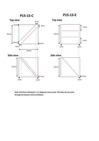
![5.2. HD-ice Target Geometry
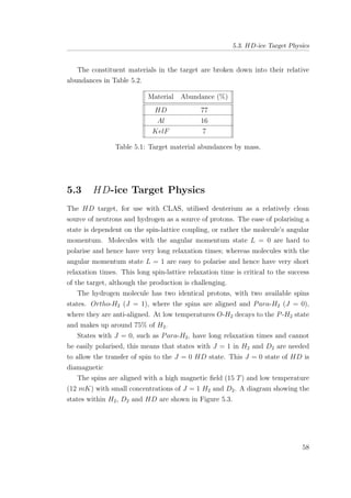
5.2 HD-ice Target Geometry
The cells used for the HDice target have dimensions of 15 mmφ × 50 mm; an
exploded-view of the target cell is shown in Figure 5.1.
Figure 5.1: Photograph of a deconstructed HDice target, showing the cell, copper
ring and Al wires [61].
The aluminium wires are used to mitigate any heat build up in the solid
HD, these are inserted into holes in a copper ring. This copper ring is double-
threaded such that it allows the cell to be transferred between dewers without
violating the magnetic field or temperature conditions. The cell walls are made
from PolyChloroTriFluoroEthylene (PCTFE - C2ClF3), also referred to as
KelF, which provides a clean cell with no background for H and D from N uclear
M agnetic Resonance (NMR) measurements. A more detailed schematic of a
constructed HD target is shown in Figure 5.2.
Figure 5.2: HD target schematic, indicating the target sizes [87].
57](https://image.slidesharecdn.com/6d482e98-273b-437a-88cf-eb4faf084ce1-161109162450/85/thesis-84-320.jpg)
![5.3. HD-ice Target Physics
Figure 5.3: Decay mechanism within the HDice target [61].
The HD molecule has a very long spin-relaxation times [88], dependent on
impurity levels in the target. Direct polarisation takes very long preparation
times, so indirect polarisation is used. A small concentration of O-H2 (of order
10−4
)1
which will readily polarise and transfer polarisation between the H in H2
and the H in HD via spin-coupling. After many O-H2 half-lives (∼ 3 months)
almost all the H2 impurity had decayed to the inert P-H2 state (1/e decay time
τ = 6.5 days), leaving the H in HD in a frozen-spin state. For D2 a similar
method is followed using a small concentration of D2. The P-D2 state has J = 1
and polarises readily like O-H2, and transfers spin to HD via spin-exchange. P-
D2 decays to O-D2 (τ = 18 days), so again after a significant number of half-lives
the D in HD will reach a frozen-spin state.
The polarisation of D will always be less than that of H due to a smaller
magnetic moment of D (µD/µH ∼ 1/3). Once polarised, the target has a beam
life of a few years due to the long relaxation time, meaning that there is no need
to ‘repolarise’ the target during running. Practically, the degree of polarisation
is given by the Brillouin function [90]:
PJ (x) =
2J + 1
2J
coth
2J + 1
2J
x −
1
2J
coth
1
2J
x ,
x =
µB
kBT
,
(5.1)
1
Impurities in the HD gas are characterised using gas chromatography and Raman
spectroscopy [89].
59](https://image.slidesharecdn.com/6d482e98-273b-437a-88cf-eb4faf084ce1-161109162450/85/thesis-86-320.jpg)
![5.3. HD-ice Target Physics
where this is dependent on the nuclear spin J, magnetic moment µ, magnetic
field B, Boltzmann constant and the temperature T. For D this is limited to
∼ 15% at 25 mK and 15 T. The characteristic curves for H and D are shown in
Figure 5.4.
Figure 5.4: Equilibrium polarisation within the HD target as a function of
magnetic field, B, and temperature, T. This shows the polarisation of hydrogen,
vector deuterium and tensor deuterium [91].
The D polarisation can be further increased by exploiting the adiabatic fast-
passage method [92] in order to transfer polarisation from H to D. The Zeeman
levels in solid HD are shown in Figure 5.5. Once the impurities of H2 and D2 are
decayed, the population of the mD = +1 and mH = +1
2
substates are greater than
the mD = −1 and mH = −1
2
substates. Forbidden RF transitions can be driven
in order to transfer state population from the initial mH = +1
2
, mD = −1, 0
states to the mH = −1
2
, mD = 0, +1 states. Employing this RF method allows
for the D polarisation to increase to up to 30%.
60](https://image.slidesharecdn.com/6d482e98-273b-437a-88cf-eb4faf084ce1-161109162450/85/thesis-87-320.jpg)
![5.4. HD-ice Target Production Equipment
Figure 5.5: Zeeman levels within solid HD [61].
During the P-H2 and O-D2 decays heat is released, which generates a problem
as the temperature must be kept low to retain polarisation. Solid HD has poor
thermal conductivity so cooling must be done by using embedded aluminium wires
in the solid HD. At low temperatures energy is transported through phonons
and experience an impedance mismatch at the HD/Al boundary, which limits
the HD temperature to around 12 mK. This method of target allows for much
shorted run times to obtain high statistics, around 75 days rather than 1000-2000
days with the previous FROST target at CLAS.
5.4 HD-ice Target Production Equipment
Production for these particular targets is a complex and time consuming process.
As such, there are many stages and various pieces of equipment involved in the
production. Specifically these need to be able to maintain low temperatures and
high magnetic fields in order to hold the target polarisation.
The following sections outline these cryogenic containers, a far more detailed
description of these can be found in [87] [93].
5.4.1 Production Dewer
The Production Dewar (PD) was used to condense the HD gas into a solid
form within the target cell. HD solidifies at temperatures of ∼ 16 K but much
lower temperatures are required to induce the polarisation required for the target.
61](https://image.slidesharecdn.com/6d482e98-273b-437a-88cf-eb4faf084ce1-161109162450/85/thesis-88-320.jpg)
![5.4. HD-ice Target Production Equipment
Once the HD gas is condensed, the PD is designed such that N uclear M agnetic
Resonance (NMR) measurements can be performed. A detailed schematic of the
PD is shown in Figure 5.6.
Figure 5.6: Schematic of the production dewar [87].
• Production Dewar Conditions: 1.5 K temperature; 2 T magnetic field.
5.4.2 Transfer Cryostat
The Transfer Cryostat (TC) was used for moving the targets between the various
dewars and cryostats. The double-threaded copper ring in the base of the target
cell, shown in Figure 5.1, allows for the maintenance of temperature and magnetic
field conditions during these transfers. One set of threads connects to the TC,
while the other links to the dewar for transfer. For example, removing a target
62](https://image.slidesharecdn.com/6d482e98-273b-437a-88cf-eb4faf084ce1-161109162450/85/thesis-89-320.jpg)
![5.4. HD-ice Target Production Equipment
from the PD using the TC: once the TC is screwed into the copper ring at the
base of the target, continuing the rotation unscrews the target from the PD. A
picture of the TC is shown in Figure 5.7.
Figure 5.7: Photograph of the transfer cryostat [87].
• Transfer Cryostat Conditions: 2 K temperature; 0.1 T magnetic field.
5.4.3 Dilution Refrigerator
The Dilution ReFrigerator (DF) was used to polarise the solid HD target. Due
to the length of target production time this was designed to hold up to three
targets at once, allowing for several targets to be produced concurrently. A
picture of the DF is shown in Figure 5.8.
63](https://image.slidesharecdn.com/6d482e98-273b-437a-88cf-eb4faf084ce1-161109162450/85/thesis-90-320.jpg)
![5.4. HD-ice Target Production Equipment
Figure 5.8: Photograph of the dilution refrigerator [87].
• Dilution Refrigerator Conditions: 10 mK temperature; 15 T magnetic field.
5.4.4 Storage Dewar
The Storage Dewar (SD) was used for the storage of target cells which were well
polarised, having spent several months in the DF. Similarly to the DF, the SD
was designed to be able to hold several targets simultaneously. The purpose of
this was to maintain the polarisation of targets before use in the experimental hall
while freeing up space in the DF so more targets could be placed into production.
• Storage Dewar Conditions: 1 K temperature; 6 T magnetic field.
5.4.5 In-Beam Cryostat
The I n-Beam Cryostat (IBC) was used to hold the target in the beam line under
conditions such that the production polarisation was maintained. It was designed
for operation in two positions: for loading from the TC (vertically) and running
inside CLAS (horizontally); these positions are shown in Figure 5.9.
64](https://image.slidesharecdn.com/6d482e98-273b-437a-88cf-eb4faf084ce1-161109162450/85/thesis-91-320.jpg)
![5.5. Full Target Production Procedure
Figure 5.9: External schematic of the IBC, shown in both the vertical (left) and
horizontal positions (right) [87].
A schematic, showing the inside of the IBC is shown in Figure 5.10.
Figure 5.10: Internal schematic of the IBC [87].
• In-Beam Cryostat Conditions: 50 − 300 mK temperature; 1 T longitudinal
magnetic field 0.07 T transverse magnetic field.
5.5 Full Target Production Procedure
Industrial standard HD gas has a purity of ∼ 98%, with ∼ 1.5% of impurities
from H2 and ∼ 0.5% of impurities from D2
2
.
To begin target production, HD gas is condensed into liquid and then to solid
in a 2-4 K production dewar. Target calibration was also done with the aid of
NMR measurements to characterise the polarisation. This is then transferred
2
This can however be purified further using a procedure developed by James Madison
University (JMU) [94], giving impurities as low as 10−4
.
65](https://image.slidesharecdn.com/6d482e98-273b-437a-88cf-eb4faf084ce1-161109162450/85/thesis-92-320.jpg)
![5.5. Full Target Production Procedure
to the dilution refrigerator using the transfer cryostat, a simple illustration of a
typical transfer is shown in Figure 5.11. The cell is then left to polarise at 15 T
and 12 mK for 2-6 months, with potentially two other targets; during this, the
HD is able to achieve a frozen spin state.
Figure 5.11: Simple illustration of a target transfer [93].
Transferring targets into CLAS is a long and careful process, as it’s important
to keep the target cooled and in a magnetic field at all times. The target is
removed from the dilution refrigerator (0.01 K/15 T) with the transfer cryostat
(2 K/0.1 T). The target is then transferred to the production dewar for a pre-run
NMR measurement (2 K/2 T) and once complete transferred to the storage dewar
(1 K/3 T). The storage dewar is then mounted onto a shock absorbing frame on
a truck and transported to Hall B. The storage dewar is then craned to level 2 of
CLAS and the target transferred to the IBC (0.2-0.7 K & 0.1-0.9 T) on level 1
and rolled into the centre of CLAS. Once the experimental runs are completed,
it is moved to the dewar for a post experiment polarisation measurement. A
diagram of this production cycle is shown in Figure 5.12.
66](https://image.slidesharecdn.com/6d482e98-273b-437a-88cf-eb4faf084ce1-161109162450/85/thesis-93-320.jpg)
![5.6. Produced Targets
Figure 5.12: The life cycle of a HDice target for use with CLAS [87].
5.6 Produced Targets
Only three targets were produced for use with production running during g14,
although others were used for beam tests. The details of these targets are
presented in Table 5.2.
Target Cell Cell Name ρ(g/cm2
) ρ wrt 21a Beam Conditions Used
21a Silver 0.028 1.0 Circularly polarised
19b Gold 0.020 0.70 Circularly/linearly polarised
22b Last 0.027 0.96 Linearly polarised
Table 5.2: Summary of the targets produced for the g14 run period and their
characteristics.
67](https://image.slidesharecdn.com/6d482e98-273b-437a-88cf-eb4faf084ce1-161109162450/85/thesis-94-320.jpg)
![6.1. g14 Overview
PeriodBeamEnergye−
BeampolRunRangeDateRangeEventsTorusCurrentTargetPol.
(GeV)(%)(106
)(A)(%)
Silver12.28181.5±1.4±3.368021−6809201/12−06/12830+1920+25.6±0.7±1.5
Silver22.28181.5±1.4±3.368094−6817606/12−11/121170+1920+23.2±0.7±1.4
Silver32.28176.2±1.4±3.168188−6823012/12−16/12250−1500+21.2±0.8±1.3
Silver42.28188.8±1.5±3.668232−6830516/12−04/01820−1500−6.4±0.4±0.4
Silver52.25888.8±1.5±3.668335−6876904/01−05/025210−1500−5.9±0.2±0.4
Gold22.54283.4±1.5±3.369227−6936410/04−18/042100−1500+26.8±1.0±1.6
EmptyA3.35688.2±1.5±3.668993−6903708/03−11/03660−15000
EmptyBb3.35688.2±1.5±3.669038−6904411/03−12/03120+19200
Table6.1:Summaryoftheg14runperiod.Thisshowseachsub-period,includingthebeam,torusandtargetcharacteristics
[95].
69](https://image.slidesharecdn.com/6d482e98-273b-437a-88cf-eb4faf084ce1-161109162450/85/thesis-96-320.jpg)
![6.2. Organisation of the g14 Data
Target 19b was substituted for the 21a target, giving a good set of runs with
highly polarised HD.
6.1.1 Estimating Target Polarisations for Periods Silver 4
and 5
Some discrepancies were raised with initial results obtained from the Silver4 and
5 periods. This manifested in a drop in the magnitude of the E observable when
compared to other periods. This indicated that the true polarisation values for
Silver4 and 5 were smaller than originally calculated using NMR measurements.
Members of the g14 group1
studied this issue using the γn → π−
p reaction, in
order to see what the target polarisation would have had to be to produce the
same E asymmetry in π−
p as seen in the Gold2 period, assuming compatible
and comparable beam helicities. The study indicated a disparity of the values
given for the target polarisation using the NMR and what was seen for the target
polarisation of the Silver4 and 5 periods.
Experimentally, at the start of the Silver4 period the target was rotated
from spin +Z, parallel to the beam momentum, to −Z anti-parallel to the beam
momentum. During this process it was noted that there were some mechanical
failures, although it is not believed that any of these issues should have caused
significant polarisation loss and it is not known why there should be any disparity
with the NMR measurement.
The result from the NMR was given as ∼ 25% whereas the analysis method
gave a target polarisation of only ∼ 6%. The true cause of this is unknown and
still being considered within the group.
6.2 Organisation of the g14 Data
Data is collected from detectors into Bank Object System (BOS) files [96]. These
contain the raw data from ADCs and TDCs taken directly from the detectors,
which can be thought of as purely binary data. In itself this information offers
no insight into properties of the detected particles as they are generally simply
a correlation of various hits within sub-detectors. The dataset is then cooked,
1
Dao Ho and Peng Peng were responsible for providing this study to the group.
70](https://image.slidesharecdn.com/6d482e98-273b-437a-88cf-eb4faf084ce1-161109162450/85/thesis-97-320.jpg)
![6.2. Organisation of the g14 Data
where it is converted into usable variables such as charge, momentum and particle
beta. The cooking was done using the CLAS reconstruction and analysis package
RECIS and was overseen by the g14 “chef”, Franz Klein.
After the cooking was completed, each detector went though a detailed
calibration procedure. These were to apply individual corrections to the data
for each subsystem; ensuring consistency across all runs and indicating potential
problems. Responsibility for these calibrations were split across the g14 group,
indicated in Table 6.2.
Calibration Responsible Prerequisite
Tagger Natalie Walford None
Time-of-Flight Haiyun Lu Tagger
Start Counter Jamie Fleming Tagger
Drift Chamber Dao Ho Time-of-flight & Start Counter
Drift Chamber Alignment Franz Klein Drift Chamber
Electromagnetic Calorimeter Irene Zonta Time-of-flight & Start Counter
Table 6.2: Calibration responsibilities and prerequisites.
Once calibration is completed the datasets are cooked once again, allowing
for the new calibration constants for all subsystems to be used. This iterative
calibration-cooking cycle is continued until the calibration of the data is of a high
standard2
and there are no misalignment artefacts in the data.
The files produced after cooking are in a compact ROOT Data Summary
Tape (DST) format, which contains banks of the physical variables allowing for
the reconstruction of events. It is these DST files which go on to be used in the
physics analysis.
The analysis for this thesis was completed using an analysis framework
based around the (C++ based) object-orientated ROOT framework from CERN
[97]. This framework is named ROOT Bank Event Extraction Routines
(ROOTBEER), which allows the reading of DST files in a form which is
independent of CLAS analysis programs and allowing analysis code to be made
2
Each sub-detector has its own requirements for a good calibration.
71](https://image.slidesharecdn.com/6d482e98-273b-437a-88cf-eb4faf084ce1-161109162450/85/thesis-98-320.jpg)
![6.2. Organisation of the g14 Data
into executables [98].
6.2.1 Data Reconstruction
If the complete experimental goals of Jefferson Lab are considered, the sheer
number of reaction channels which are of interest is staggering, meaning that
often very wide and generic triggers are used to record events3
. When one channel
is considered for analysis, the volume of other events contained within the data
are considerable in scale. It is completely impractical to run an analysis over the
entire dataset in terms of computational time alone. It is much more productive
to remove the extraneous data to massively reduce the size of the set, this practice
is called skimming; the channel of interest can then be identified with much less
processing time. These skims can be set up for exclusive final states, such as
K+
Σ−
, or much more generic inclusive final states, such as K+
X.
Events are reconstructed from the basic data acquired from detector subsys-
tems. Arrays of measurable quantities for each particle are obtained from the
various detectors; these are used to describe the particle properties during the
reconstruction, with variables such as charge, mass, momentum and velocity.
6.2.1.1 Particle Charge and Momenta
The charge of a particle can be ascertained from the interaction of the particle
with the magnetic field of the drift chambers. The direction of the curvature
identifies whether the particle charge is positive or negative; neutral particles will
be unaffected by the magnetic field.
A particle can be described using the Lorentz force:
F = q[E + (v × B)], (6.1)
where F is the Lorentz force acting on the particle, of charge q moving with
velocity v in the presence of an electric field E and a magnetic field B. In
the case of the CLAS drift chambers, the electric field is absent so this can be
simplified to:
3
The trigger at CLAS consists of two levels. Trigger Level 1 processes all prompt (90 ns)
signals, with a more robust Level 2 trigger which requires a candidate for a track in the DC.
72](https://image.slidesharecdn.com/6d482e98-273b-437a-88cf-eb4faf084ce1-161109162450/85/thesis-99-320.jpg)
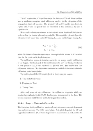
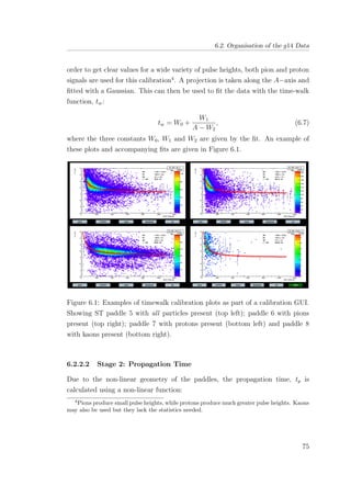
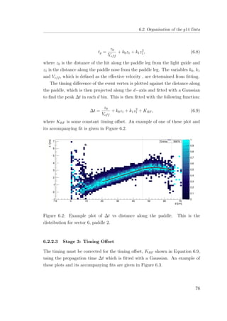
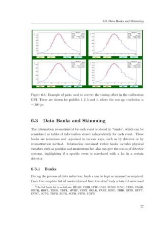
![6.3. Data Banks and Skimming
in the final analysis, although others were useful for diagnostic purposes. The
main bank used in the analysis was the GPID bank [99].
The GPID bank contains particle information, as well as information from the
time-of-flight scintillators, start counter and tagger. Initially during the selection
the Particle IDentification (PID) variable of this bank was used as some initial
particle selection, though this is not a very robust method. The PID variable
was mainly considered for some initial diagnostic tests and was later dropped in
favour of a more robust method of selection.
The PID variable is defined as follows; the momentum is determined from the
bending of the particles in the DC magnetic field. From this, values of the particle
β are trialled using the PDG particle masses. The value of β is measured using
time-of-flight information and the difference between these measured values and
the trail values are minimised. This best suited identity is then assigned to the
particle. This method has associated issues, paricularly when particle corrections
are not taken into account and particularly struggles to separate pions and kaons
at high momenta.
Other banks used in this analysis are outlined below:
• HEAD: Bank containing information about the run; primarily used to
obtain the number of the current run.
• MVRT: Bank containing information about the event vertex.
• TBID: Bank containing information about time-based particle ID; us-
ing details from the time-of-flight, Cherenkov counter, electromagnetic
calorimeter, start counter and large angle calorimeter.
• TAGR: Bank containing information from the photon tagger; primarily used
for the selection of the event photon.
6.3.2 K+
Σ−
Skim
The skim used in this analysis was an exclusive K+
Σ−
skim. The particle
identification for charged tracks were taken from the EVNT or PART banks of
CLAS, and selecting particle β using momentum p (in GeV ): βmin < β < βmax.
The full requirements of the K+
Σ−
skim were as follows:
78](https://image.slidesharecdn.com/6d482e98-273b-437a-88cf-eb4faf084ce1-161109162450/85/thesis-105-320.jpg)
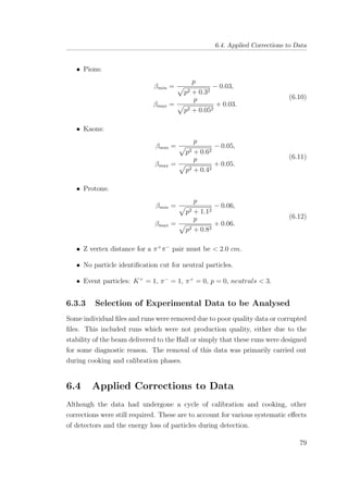
![6.4. Applied Corrections to Data
6.4.1 Kinematic Fitting
The goal of using a correction to particle momentum is to improve the resolution
of the data; for the g14 period this was done using kinematic fitting [76] [100].
A measured quantity, the particle 4-vector, must fulfil certain kinematic
constraints, such as the conservation of momentum. Since these measured
quantities have some associated uncertainty, the constraints are not perfectly
satisfied. The constraint boundaries can then be used to slightly change the
measured values, within the parameters of their uncertainties, without breaking
conservation.
The goal of kinematic fitting is to have an event-by-event least squares fitting
to ensure the measured values fulfil the constraints. The software used for this
iterative procedure was developed at Carnegie M ellon U niversity (CMU).
Least squares fitting, utilises the minimisation of the sum of the squares of
the data offsets from some fit, commonly referred to as residuals. If we consider
the sum of the residuals for a set of n points for some function f:
R2
=
i
[yi − f(xi, a1, a2, ..., an)]2
, (6.13)
where yi is the measured value for each of the n events.
The sum of the squares is used so we can exploit the fact that the residuals
can be treated as a continuous differentiable quantity. This does mean however
that outlying points are given disproportionately large weighting due to the
construction of R2
. The condition to minimise R2
for some dataset i = 1, ..., n is:
∂(R2
)
∂ai
= 0. (6.14)
If some measurable quantity is considered, we can write:
−→η = −→y + −→, (6.15)
where −→y are the estimator variables as given by a fit and −→ are the set of
deviations needed to shift the observed values of −→η to satisfy the constraints.
Ideally these shifts in −→η should have a Gaussian distribution around zero. The
shift distributions are checked at each iteration, which is done by using pull
distributions in order to measure the relative difference of the values and their
80](https://image.slidesharecdn.com/6d482e98-273b-437a-88cf-eb4faf084ce1-161109162450/85/thesis-107-320.jpg)
![6.4. Applied Corrections to Data
uncertainties, reminiscent of the residuals. The pulls are defined as:
z =
ηit − yit
σ2
ηit
− σ2
yit
. (6.16)
The iterations continue until they converge on an ideal Gaussian distribution,
µ = 0; σ2
= 1.
6.4.2 CLAS tracking parameters
Three separate coordinate systems are used in CLAS. These are the tracking
system, lab system and sector system. It is important to consider the transition
from the tracking system to the lab system within CLAS for use with the
correction methods. The track system defines x along the beam line; y through
the sector centre and z along the average magnetic field direction. Whilst the lab
system defines the x through the centre of sector 1; y is vertically upwards and z
is along the direction of the beam line. These systems are shown in Figure 6.4.
Figure 6.4: Diagram outlining the two coordinate systems used in CLAS [63].
The track system can be related to the lab system as follows:
81](https://image.slidesharecdn.com/6d482e98-273b-437a-88cf-eb4faf084ce1-161109162450/85/thesis-108-320.jpg)
![6.4. Applied Corrections to Data
xtrack
ytrack
ztrack
=
zlab
cos(α)xlab + sin(α)ylab
− sin(α)xlab + cos(α)ylab
, (6.17)
where α = π
3
(Nsector − 1).
The momenta of the tracks are considered in terms of the ratio of momentum
and charge, q/|p|, the dipolar angle relative to the sector plane, λ and the angle
in the sector plane relative to the xtrack axis, φ [101]:
pxlab
pylab
pzlab
=
p(cos(λ) sin(φ) cos(α) − sin(λ) sin(α))
p(cos(λ) sin(φ) sin(α) + sin(λ) cos(α))
p cos(λ) cos(φ)
. (6.18)
6.4.3 Energy Loss Correction
CLAS uses the curvature of charged particle tracks in the DC to determine
particle momentum. However the code used during the reconstruction does not
take into account the energy loss due to material the particle encounters before
it reaches the drift chambers. This becomes critically important for photon runs
as the start counter is placed surrounding the target, removing yet more energy.
This is particularly important for low momentum particles which lose their energy
easily. The Eloss software6
attempts to correct for these energy losses.
From the event vertex to the drift chambers, the particle must pass through
a significant amount of material such as the start counter paddles, beam pipe
and target cell material/wall. The software looks at the path of the particle to
identify which materials it has passed through. The thicknesses of the various
materials are calculated and the software attempts to correct the 4-vector for the
energy which would be lost in the material. Although this has been done for many
previous experiments at CLAS, the software target was updated specifically for
the HDice target geometry and material [102].
6
The Eloss software was written and updated for the g14 run by Eugene Pasyuk of Jefferson
Lab.
82](https://image.slidesharecdn.com/6d482e98-273b-437a-88cf-eb4faf084ce1-161109162450/85/thesis-109-320.jpg)
![6.4. Applied Corrections to Data
6.4.4 Momentum Correction
Several factors lead to the need for momentum corrections after the calibration
phase. The CLAS reconstruction momentum is taken from DC information;
which means that any errors in the alignment of the DC or inaccuracies in the
field map will be propagated into the reconstructed momenta. The reaction
γp → pπ+
π−
was studied to obtain the corrections. The Eloss correction was
applied to the final state particles before the event was kinematically fitted. The
correction works in terms of considering three hypotheses; wherein one of the
final state particles is considered “missing”:
• γp → (p)missingπ+
π−
,
• γp → p(π+
)missingπ−
,
• γp → pπ+
(π−
)missing.
The corrections applied are:
∆px = pkfit
x − pmeas
x ,
∆λx = λkfit
x − λmeas
x ,
∆φx = φkfit
x − φmeas
x ,
(6.19)
where p is the magnitude of the momentum vector; λ is the dipolar angle relative
to the sectors (x, y) for the track and φ is the the angle of the xtrack relative to
the (x, y) plane.
6.4.5 Tagger Correction
An additional correction must be added to the tagger after calibration, as
alignment issues lead to photon energies being reconstructed with some offset
[101]. This misalignment comes from the weight of the paddles over time moving
them from their original alignment, leading to inaccurate values given by certain
tagger channels. Note that these corrections will also differ according to the
energy of the electron beam and so must be considered for each beam setting. The
reaction γp → pπ+
π−
was again studied after the Eloss correction was applied.
The events were then kinematically fitted, and events with a Confidence Level
83](https://image.slidesharecdn.com/6d482e98-273b-437a-88cf-eb4faf084ce1-161109162450/85/thesis-110-320.jpg)
![6.4. Applied Corrections to Data
(CL) greater than 10% were used to determine the correction. The correction for
each beam energy, Ebeam is:
∆Etag =
Ekfit
γ − Emeas
γ
Ebeam
, (6.20)
where Ekfit
γ is the photon energy value from the kinematic fitting and Emeas
γ is
the photon energy from the tagger system. The correction was then used for the
associated beam period and then for each tagger paddle on an event-by-event
basis.
6.4.6 Neutron Vertex Correction
If the neutron was able to be reliably detected and the complete final state K+
π−
n
identified, more corrections would need to be made. This consideration is not
required for this work but would become important during any higher statistics
experiments.
Neutrons are detected finally in the CLAS EC. Due to the large interaction
length for the neutron in the EC, it is difficult to accurately pinpoint the hit
coordinates. Any offsets in the interaction vertex within the EC can be considered
using a careful study of the channel γD → π+
π−
pn. This takes advantage of
a common production vertex, therefore giving a reliable neutron vertex in the
target.
When considering the K+
Σ−
channel rather than π+
π−
pn, there is a subtlety.
The neutron that we would consider has a displaced vertex as the decay length of
the Σ−
is ∼ 4.43cm. Though generally when CLAS assigns vertex it chooses the
vertex of the fastest particle in the event (e.g. a fast π±
). This is usually a good
approximation when the neutron comes from the primary interaction vertex, but
something more subtle would have to be considered and studied to have some
idea what influence this vertex choice would have in the data.
These neutron corrections were implemented in the previous measurements in
CLAS [54] [60].
84](https://image.slidesharecdn.com/6d482e98-273b-437a-88cf-eb4faf084ce1-161109162450/85/thesis-111-320.jpg)
![Chapter 7
γN → K+Σ− Event Selection
This chapter details the use of the g14 period dataset to reconstruct and identify
the reaction yield of:
γn → K+
Σ−
→ K+
π−
n. (7.1)
7.1 Outline
The g14 experiment is one of the first measurements of the photoproduction of
mesons from a polarised neutron target and will be instrumental in the world
programme to better establish the excitation spectrum of the nucleon. Expected
rates are given in [61] as ratios to other decay channels. It is expected that the
cross section of K+
Σ−
is one fifth of the cross section of K0
Λ. An estimate of
K0
Λ was made by JLab of 104
events for the experimental period, giving 2000
expected events for K+
Σ−
. It has since been thought that this initial ratio of
1 : 5 is a large underestimate, from a relative comparison of other run periods.
Previous experiments at JLab have shown that this ratio may be much closer
to 1 : 11
. Since this was clearly uncertain, a rough event study was undertaken
before the full analysis was initiated. This study confirmed that enough events
were present to warrant a complete analysis.
This channel is particularly challenging for several reasons other than the low
relative cross section. Firstly, power of the polarisation observable measurement
is correlated with the available target polarisation, which was predicted to be able
1
From private correspondence with Franz Klein.
85](https://image.slidesharecdn.com/6d482e98-273b-437a-88cf-eb4faf084ce1-161109162450/85/thesis-112-320.jpg)
![7.2. Event Selection
to have values of 75% for H and 40% for D. In practice typical values of 15-25%
were obtained for both H and D. Secondly, CLAS itself was not designed as a
neutral particle detector, with a neutron efficiency of only 5-7% [61], so with a
final state neutron this becomes problematic. Misidentification is also a concern,
specifically the false ID of K+
as π+
. Finally, because the target neutron is bound
inside deuterium, from this bound state inside the deuteron there will be Fermi
motion of the nucleon.
7.2 Event Selection
After the data is skimmed, as outlined in Section 6.3.2, the files were transferred
to a storage space at the University of Edinburgh. These individual run files
were arranged and merged into periods as outlined in Table 6.1. Once this was
complete the event selection procedure could begin. Each stage of selection was
carefully monitored in terms of statistics of events removed, in order to ensure
sensible reductions.
7.2.1 Coarse Data Reduction
The skimmed CLAS data contains the events of interest, as well as other reaction
channels not studied in this thesis. Initial coarse selection cuts were applied to
the skimmed data to further reduced the data sample.
The multiplicity of an event is the number of particles successfully identified
in the final state. Of course, ideally for this analysis all three final state particles
would be identified, K+
π−
n. However, due to the restrictions of CLAS to identify
neutral particles this is not always possible. This means that the two particles,
non-exclusive, final state, K+
π−
, where the neutron has not been detected
is the primary consideration. For this case the (undetected) neutron can be
reconstructed from the missing mass : γn → K+
π−
X. Mx can be evaluated on
an event-by-event basis to select neutron candidates from the reaction yield.
By considering the hit multiplicity in CLAS and selecting events with two and
three particle final states we can reduce the data to be processed. Furthermore
we can improve the quality of the data selected by requiring that events also have
a valid hit in the tagger. The distribution of the selected final states are shown
in Figure 7.1:
86](https://image.slidesharecdn.com/6d482e98-273b-437a-88cf-eb4faf084ce1-161109162450/85/thesis-113-320.jpg)
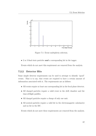
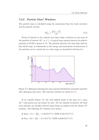
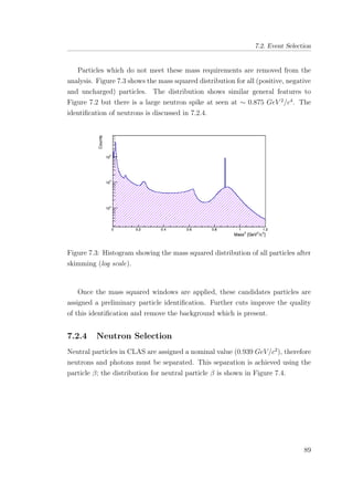
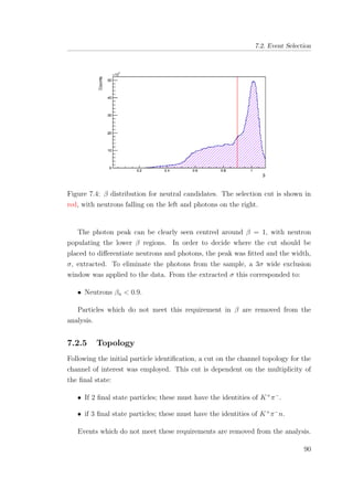
![7.2. Event Selection
7.2.6 Momentum vs ∆β
Further refinements to the particle ID are carried out by utilising the correlation
between the independently measured momentum (from the DC) and the measured
time-of-flight (from the SC). The momentum vs β distribution for positive and
negative particles is shown in Figure 7.5. The proton and pion bands are clearly
seen in red, while the kaons can be made out in between. The other bandings,
having a more horizontal locus, can be attributed to misidentified particles. The
shadows in the bands (i.e. a mirror band occurring at a different β) are attributed
to events where the photon was taken to be from the wrong beam bucket and as
the time-of-flight was calculated by using an incorrect start time. The error in
the momentum from the track curvature is of the order of ∼ 1%, while in β it
is up to ∼ 5% as the uncertainty comes from the time-of-flight and path length
[67].
Figure 7.5: Momentum vs β distribution for positive and negative particles (log
scale).
Figure 7.5 shows that at higher momenta the kaon and pion candidates
begin to converge, particularly at > 1.5 GeV/c. At these higher momenta their
separation becomes difficult due to the worsening β resolution and the proximity
of their loci.
To allow more simple particle ID regions to be identified, it is useful to present
91](https://image.slidesharecdn.com/6d482e98-273b-437a-88cf-eb4faf084ce1-161109162450/85/thesis-118-320.jpg)
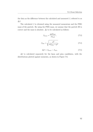
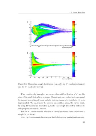
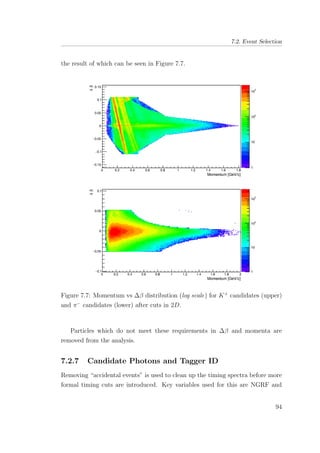
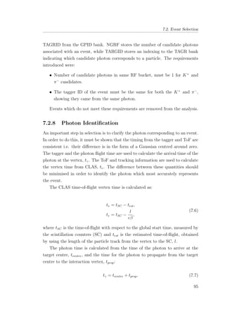
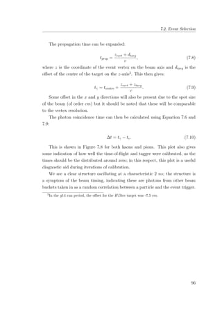
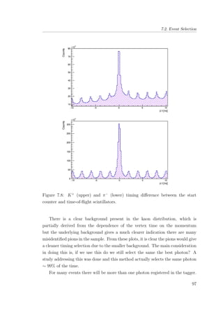
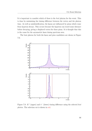
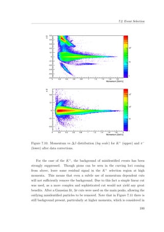
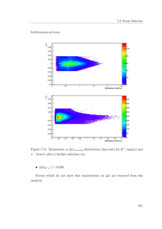
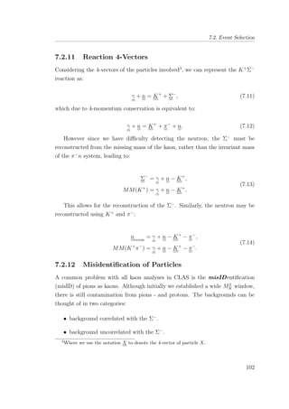
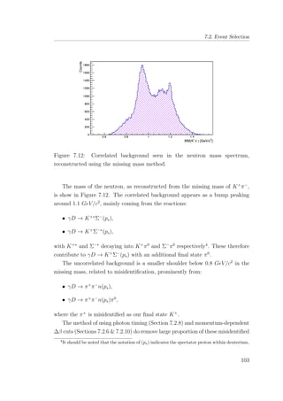
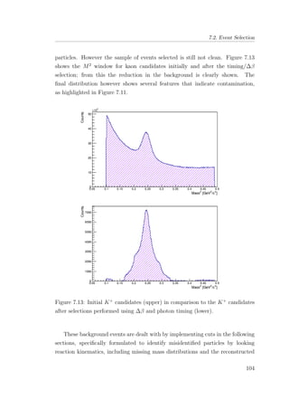
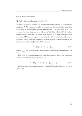
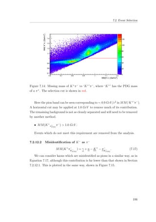
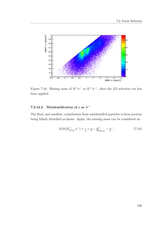
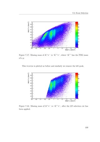
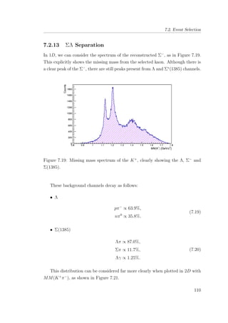
![7.2. Event Selection
Figure 7.20: 2D plot of the reconstructed Σ−
[MM(K+
)] vs. the reconstructed
neutron [MM(K+
π−
)].
In this plot, the Σ−
(PDG 1198 MeV ) can be seen; in addition the Λ (PDG
1116 MeV ) is also present at lower mass, although clear separation can only be
seen in 2D. Considering the 2D distribution also clearly shows a contribution
from Σ0
(PDG 1193 MeV ), where there is an additional π0
in the final state.
The Σ0
decays as follows:
• Σ0
Λγ ∝ 100%. (7.21)
The Σ−
can then be isolated using a linear cut in 2D, to remove contributions
from Λ and Σ0
. The distribution after this cut is shown in Figure 7.21.
111](https://image.slidesharecdn.com/6d482e98-273b-437a-88cf-eb4faf084ce1-161109162450/85/thesis-138-320.jpg)
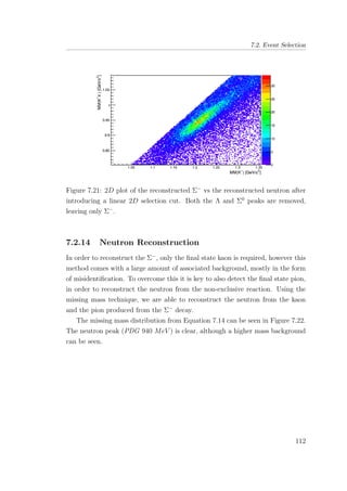
![7.2. Event Selection
Figure 7.22: Reconstructed neutron using the missing mass technique
[MM(K+
π−
)] after misID selections have been applied.
The nature of this background is clearer when presented in 2D versus
momentum of the K+
, Figure 7.23. The neutron peak was fitted with a Gaussian,
in 1D, and σ extracted. A study was undertaken to show affect of varying σ
around this peak5
.
5
After the study was concluded a selection cut of 2σ was chosen.
113](https://image.slidesharecdn.com/6d482e98-273b-437a-88cf-eb4faf084ce1-161109162450/85/thesis-140-320.jpg)
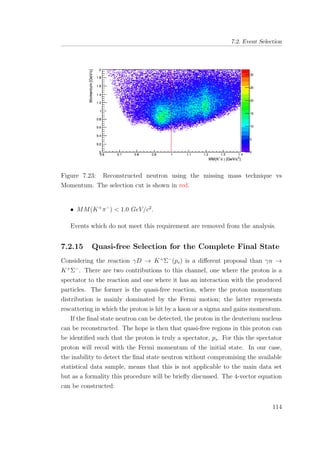
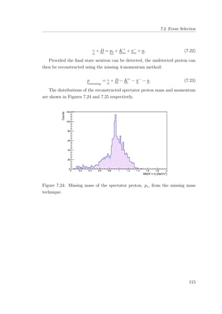
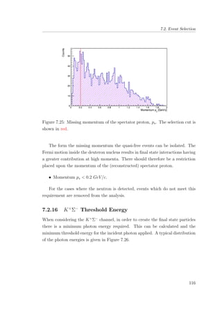
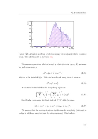
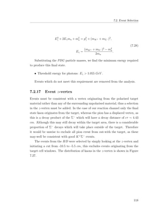
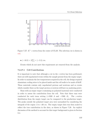
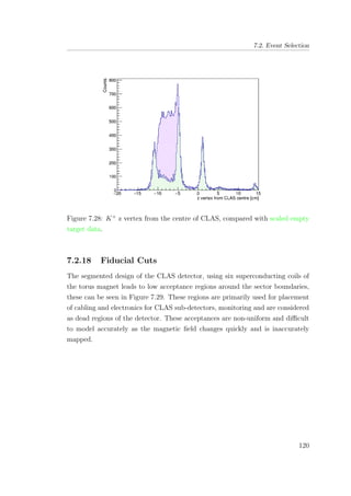
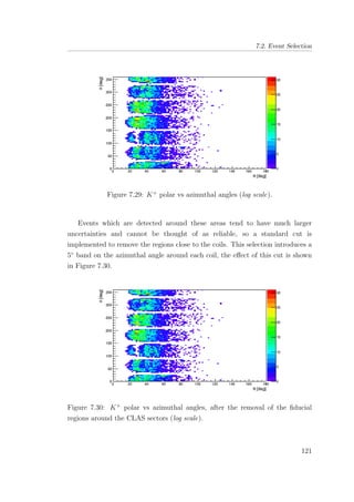
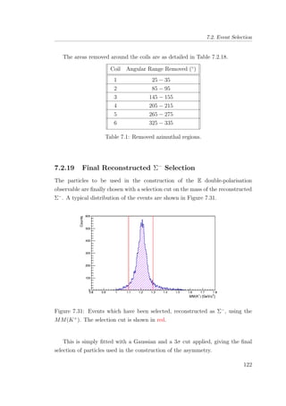
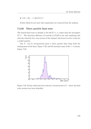
![7.2. Event Selection
Figure 7.33: Reconstructed Σ−
, using the invariant mass method [M(nπ−
)].
Comparing these plots to the final selection in the two particle final state,
we find a difference in statistics of a factor ∼ 20. This would be a preferable
final state to analyse, in terms of minimising background and taking advantage
of the ability to use the invariant mass, as has been done in measurements of the
cross section [60], however the statistics available for this work does not make
this viable.
7.2.21 Summary
A summary of the applied selection cuts and corrections in this chapter are
outlined below.
124](https://image.slidesharecdn.com/6d482e98-273b-437a-88cf-eb4faf084ce1-161109162450/85/thesis-151-320.jpg)
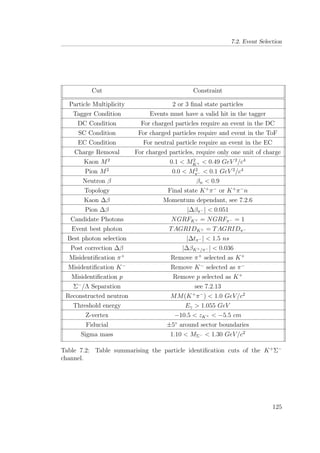
![Chapter 8
Extraction of Polarisation
Observables
This chapter outlines the extraction of the double-polarisation observable E for
the reaction γn → K+
Σ−
from the g14 experimental data.
8.1 Introduction
The polarised cross section, dσ
dΩ
, is related to the unpolarised cross section, (dσ
dΩ
)0,
by:
dσ
dΩ
=
dσ
dΩ 0
(1 − PγP⊕E), (8.1)
where Pγ is the polarisation of incident photon and P⊕ is the polarisation of the
target. The observable E can be extracted from the beam-asymmetry [103], A,
which is defined as:
A =
N1
2
(→⇐) − N3
2
(←⇐)
N1
2
(→⇒) + N3
2
(←⇒)
, (8.2)
where N represents the appropriate number of events for the corresponding target
(→) and beam (⇒) polarisation vectors. The beam-asymmetry is then used in
conjunction with the target and photon polarisations to give an expression for
the double-polarisation observable E:
126](https://image.slidesharecdn.com/6d482e98-273b-437a-88cf-eb4faf084ce1-161109162450/85/thesis-153-320.jpg)
![8.2. Angle and Energy Bin Choice
E =
1
PγP⊕
A. (8.3)
8.2 Angle and Energy Bin Choice
The extraction of the E observable from the γn → K+
Σ−
reaction is considered
as a function of Eγ (lab frame) and cosθCM
K+ (centre-of-mass frame).
Figure 8.1: Diagram showing the kinematics for the γn → K+
Σ−
in the centre-of
mass frame [54].
The binning of each of these must be carefully chosen. There are were two
possibilities considered:
• Bin according to some standard spacing of bin centres.
• Bin according to equal bin statistics.
In the first case, some bins can suffer from very low statistics and therefore
be of little use in terms of analysing power. In the second case, bins are
often asymmetric and may be problematic when integrating over large intervals.
Therefore it can be seen that there is a balance to consider between these two
binning methods.
127](https://image.slidesharecdn.com/6d482e98-273b-437a-88cf-eb4faf084ce1-161109162450/85/thesis-154-320.jpg)
![8.2. Angle and Energy Bin Choice
8.2.1 Eγ Binning
The binning in Eγ, was chosen to be 200 MeV . This was chosen after considering
the total statistics available to the channel. Although more bins are preferable,
this would mean that the errors within each Eγ bin would be considerably
larger. Fortunately, the E observable does not evolve quickly in terms of photon
energy and at the scale of 200 MeV there is limited movement. The asymmetry
predictions are considered explicitly in Section 8.9. The full photon energy
spectrum is shown in Figure 8.2.
Figure 8.2: Energy spectrum of photons, after all event selections have taken
place. The binning is shown in red.
The photon energy bins chosen are shown in Table 8.1, along with the
respective statistics of each bin.
8.2.2 cosθCM
K+ Binning
The binning in cosθCM
K+ was selected using symmetric bins over the complete
angular range of θCM
K+ (cos θCM
K+ ) = [−1, 1]. Again, due to statistics a relatively
small number of angular bins were selected. Five angular bins per photon energy
were used to extract the measurement of E. The distribution of cos θCM
K+ over all
energies is shown in Figure 8.3.
128](https://image.slidesharecdn.com/6d482e98-273b-437a-88cf-eb4faf084ce1-161109162450/85/thesis-155-320.jpg)
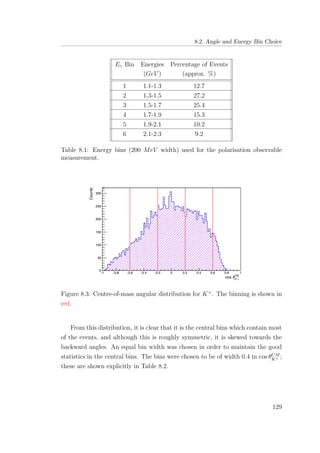
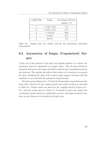
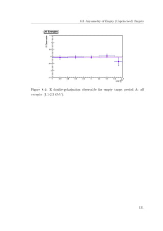
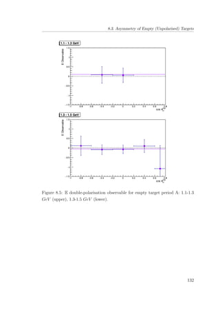
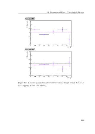
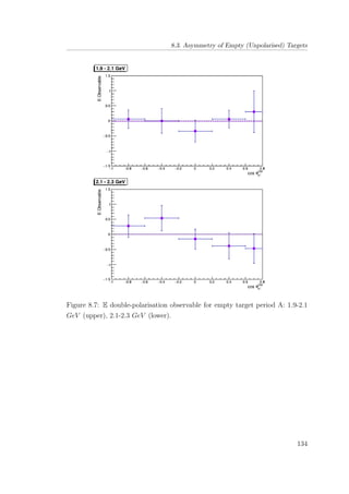
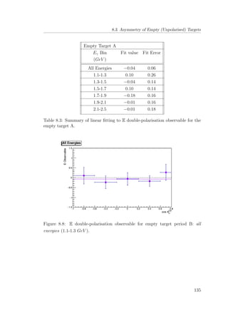
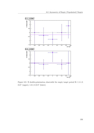
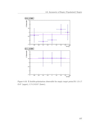
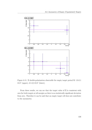
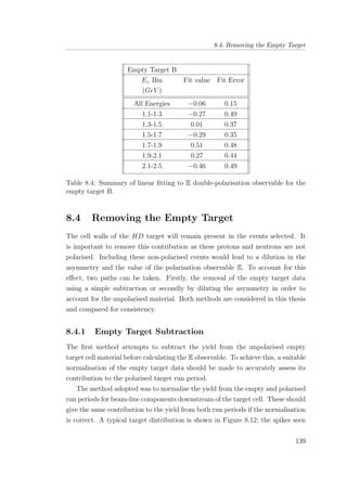
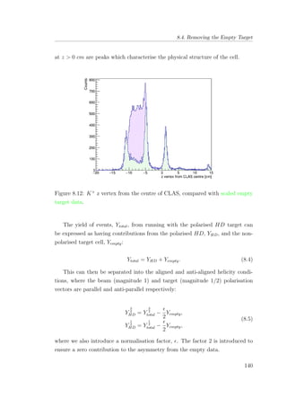
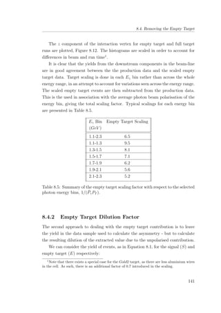
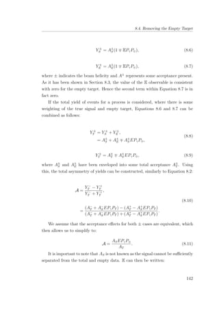
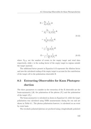
![8.6. Investigation of Systematics in Extraction of the Asymmetry
electron beam, incident on a bremsstrahlung radiator. The degree of polarisation
depends on the ratio of energies x = Eγ/Ee− . This ratio allows for calculation of
the polarisation of the incident photon [75]:
Pγ = Pe−
4x − x2
4 − 4x + 3x2
. (8.14)
The degree of photon polarisation is considered separately in each energy
bin as there is a photon energy dependence that must be accounted for. So
the mean value of photon polarisation is taken for each bin. The evolution of
photon polarisation with photon energy is shown in Figure 8.13, while the photon
polarisation for each energy bin is considered in Table 8.6.
Figure 8.13: Photon energy (Eγ) vs photon polarisation.
8.6 Investigation of Systematics in Extraction
of the Asymmetry
This section presents results from investigations into potential systematics in
the extraction of the asymmetry, A, arising from detector acceptance effects.
The extracted value for the asymmetry should not show any dependence on the
azimuthal angle of the reaction products. This lack of dependence on φ was
checked using the final state kaon in the analysis presented below.
144](https://image.slidesharecdn.com/6d482e98-273b-437a-88cf-eb4faf084ce1-161109162450/85/thesis-171-320.jpg)
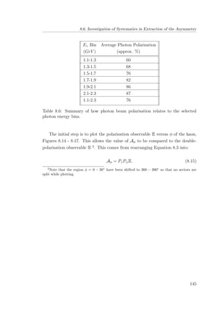
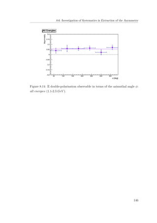
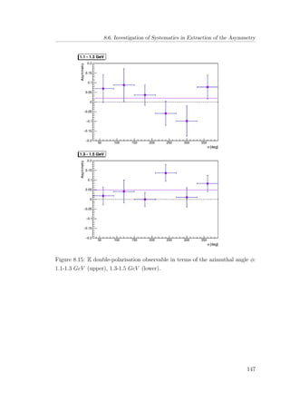
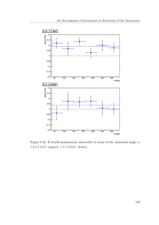
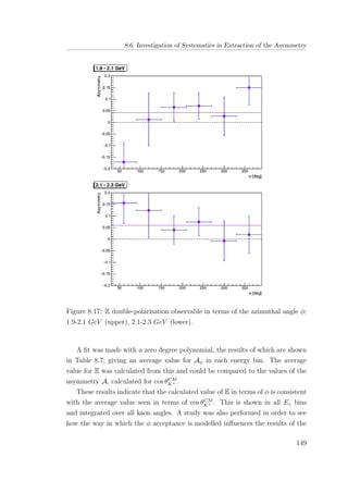
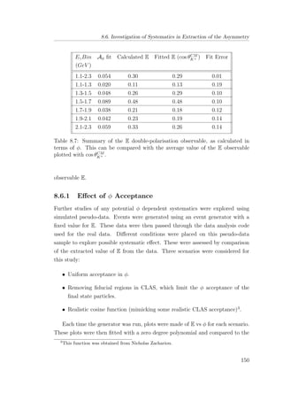
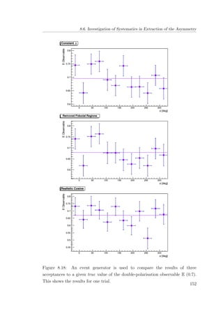

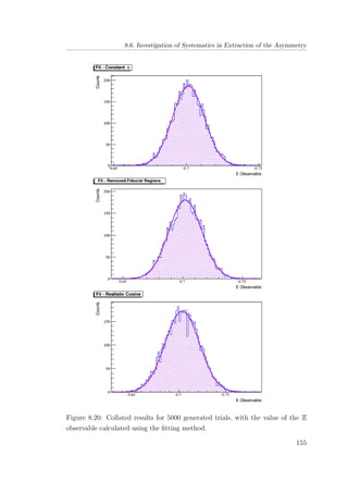
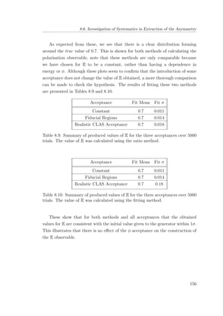
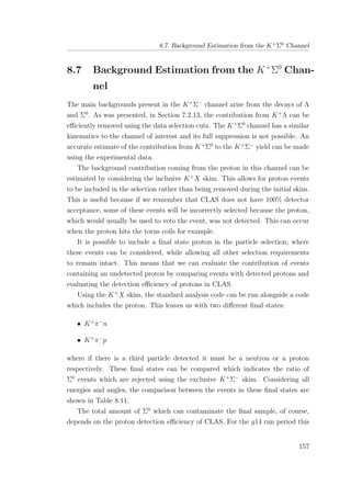
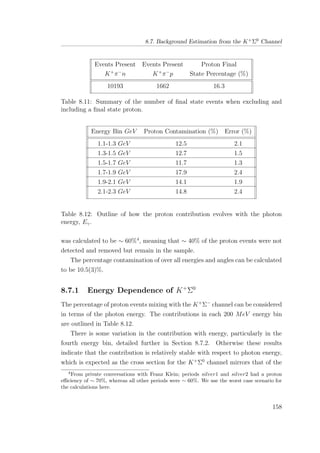
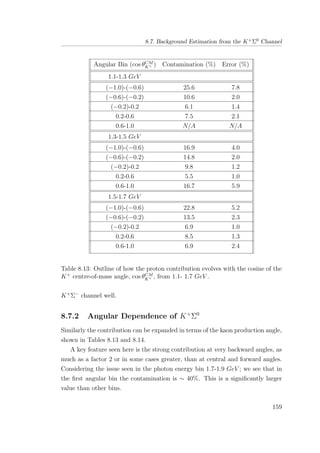
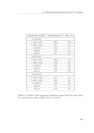
![8.8. Combining Period Results
An estimation of the background is included in the systematic error estimate
for the final results.
8.8 Combining Period Results
The Gold2 and Silver periods were combined into one complete dataset in
order to improve the statistics for calculating the beam-asymmetry and therefore
the errors of the observable E. It is important to ensure that these periods
are appropriately weighted when they are combined as each will have differing
statistics. This can be thought of as weighting the value of the polarisation
observable in accordance with the error on the value; i.e. imprecise values with
large errors are thought of as less reliable while more accurate values with smaller
errors are weighted more heavily.
A weighted mean was used when periods were combined to ensure that
contributions from each target period are appropriately accounted for. For a
set of data, [x1, x2, ..., xn], the weighted arithmetic mean is written as:
¯x =
n
i=1
wixi
n
i=1
wi
, (8.16)
where wi is the variable which is being used to weight the data5
.
8.9 Current Theoretical Model Prediction
The two models used as a comparison in this thesis were KaonMAID, and
Bonn-Gatchina. Although the MAID prediction has not been updated since its
calculation in 2000, it is one of the few models to actually include the K+
Σ−
reaction.
The plots of the polarisation observable E, use two theoretical predictions for
each model. These are added because bins are relatively wide (200 MeV ) due to
the low statistics available. The predictions shown are the bin end points with
5
In our case, the number of events in the target period is used to represent the analysing
power of each period.
161](https://image.slidesharecdn.com/6d482e98-273b-437a-88cf-eb4faf084ce1-161109162450/85/thesis-188-320.jpg)
![8.9. Current Theoretical Model Prediction
the upper shown in red and lower in blue. This clearly highlights the evolution
of the E observable prediction across the width of the energy bin.
8.9.1 KaonMAID
Predictions from the KaonMAID model [104] evolving with photon energy are
shown in Figures 8.21 and 8.22.
Figure 8.21: Predictions from KaonMAID for E in the reaction γn → K+
Σ−
.
These are plotted every 100 MeV : 1050, 1150, 1250, 1350, 1450, 1550.
162](https://image.slidesharecdn.com/6d482e98-273b-437a-88cf-eb4faf084ce1-161109162450/85/thesis-189-320.jpg)
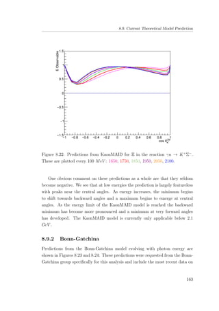
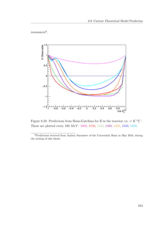
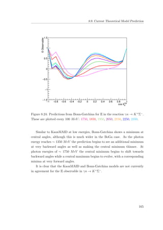
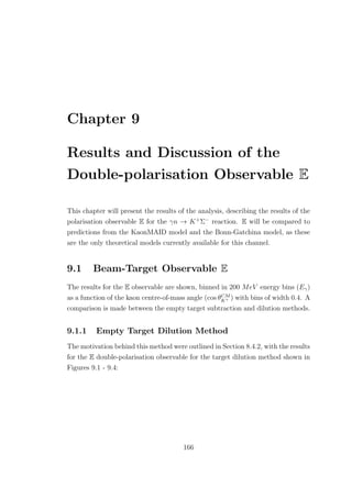
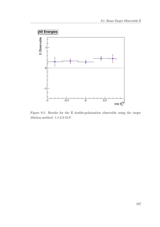
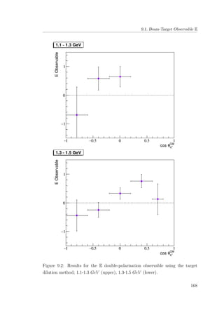
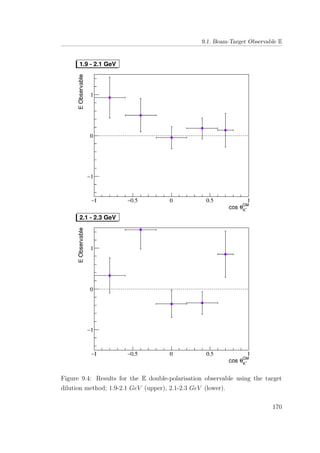
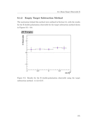
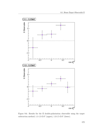
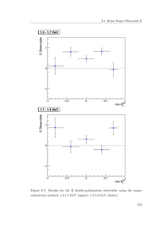
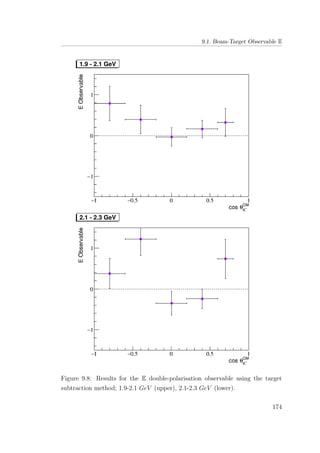
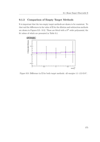
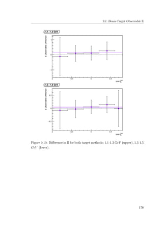
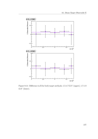
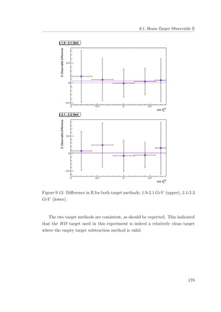
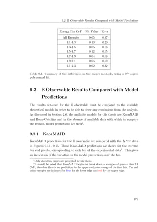
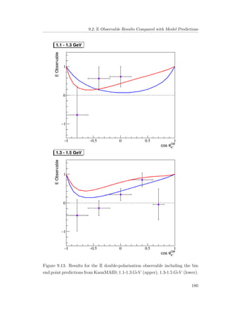
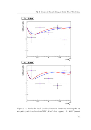
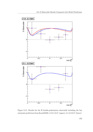
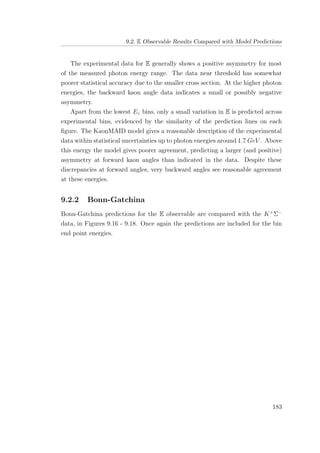
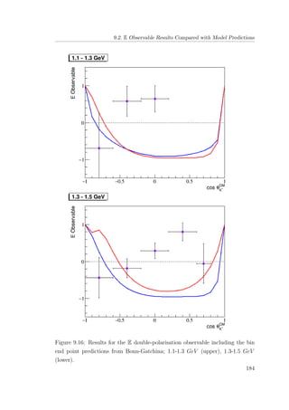
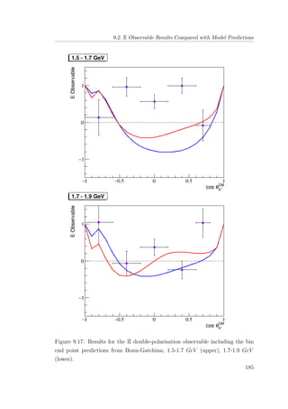
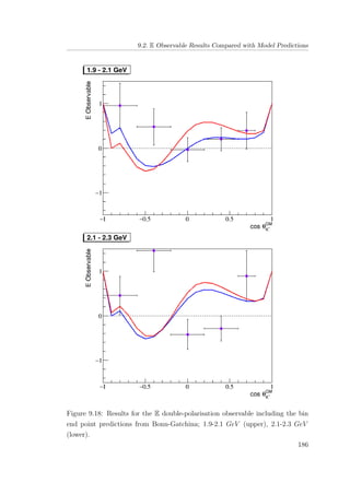
![9.3. Systematic Uncertainties
Contribution to polarisation systematic σsys
Photon Beam Polarisation 3.4%
Target Polarisation 6.0%
Total 6.89%
Table 9.2: Systematic uncertainties associated with polarisation measurements
during the g14 run period.
The Bonn-Gatchina predictions do not show very significant variation across
the experimental bins, with predictions from the bin edges indicating similar
trends and magnitude. The Bonn-Gatchina model predicts more negative
asymmetries than KaonMAID for photon energies below 1.7 GeV . This behaviour
is not well reflected in the data, as we see a clear difference in sign between
the model and data at central kaon angles. At higher photon energies the
smaller predicted asymmetries show better general agreement with the data
within uncertainties. The Bonn-Gatchina model is constrained by a much larger
database including recent meson photoproduction data, so this poorer agreement
is interesting.
9.3 Systematic Uncertainties
Two kinds of systematic uncertainties were considered. Firstly, those associated
with event selection and observable extraction. Secondly, those systematic
uncertainties associated with the presence of the K+
Σ0
background channel were
assessed on a bin-by-bin basis.
The systematic error associated with the empty target subtraction was taken
to be negligible compared to the statistical error, from the agreement between
different analysis methods, shown in Section 9.1.3. Systematics in the measured
photon flux are assumed to cancel in the asymmetry and to be of similar
magnitude for both helicities. There was no significant variation in the asymmetry
found when varying the particle selection cuts, these were found to be consistent
within uncertainties.
Systematic uncertainties of the photon and target polarisations were calcu-
lated by the g14 run group [105]. These are shown in Table 9.2.
187](https://image.slidesharecdn.com/6d482e98-273b-437a-88cf-eb4faf084ce1-161109162450/85/thesis-214-320.jpg)
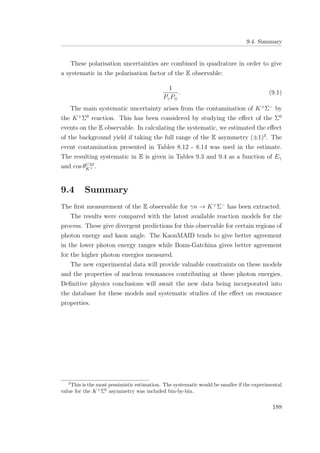
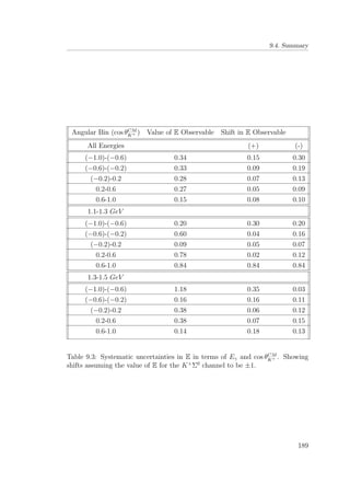
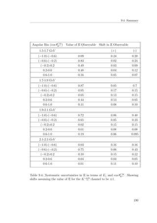
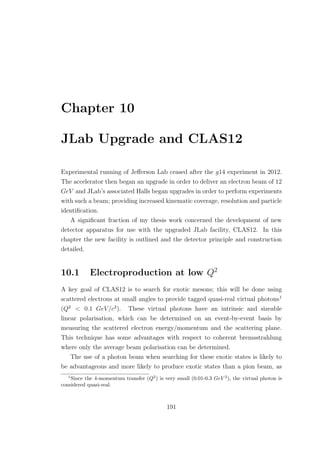
![10.1. Electroproduction at low Q2
the use of a spin − 1 probe may favour production of q¯q states where the quark
spins are aligned which is more likely to provide a meson with exotic quantum
numbers [106]. Phenomenological studies also suggest that the cross section of
these exotic states would be comparable to non-exotic mesons [107] [108].
The use of low Q2
allows a more controlled use of photon flux, so thin targets
can be used. This method is expected to have a luminosity of 1035
cm−2
s−1
with
a tagged photon rate of 107
s−1
[67]. This technique has been used to produce
very high energy photon beams at CERN [109] [110] and DESY [111].
The use of unpolarised electrons, allows for a virtual photon to be produce
with polarisation:
= 1 + 2
(Q2
+ ν2
)
Q2
tan2
(θe /2)
−1
, (10.1)
where ν is the photon energy and θe is the scattering angle of the electron [112].
The longitudinal polarisation is given by;
L =
Q2
ν2
. (10.2)
At very small values of Q2
, the virtual photons are seen as quasi-real since
L ≈ 0. From measurements made of the scattered electron, properties of the
quasi-real photon can be reconstructed. Three key quantities are required for the
correct determination of polarisation; firstly, the azimuthal angle φe , in order to
determine the polarisation plane. Secondly, the energy of the scattered electron
for the calculation of linear polarisation:
ν = Ebeam − Ee ,
Pγ = 1 +
ν2
2EbeamEe
.
(10.3)
Finally, the polar angle, θe , to determine the momentum transfer:
Q2
= 4EbeamEe sin2
(θe /2). (10.4)
192](https://image.slidesharecdn.com/6d482e98-273b-437a-88cf-eb4faf084ce1-161109162450/85/thesis-219-320.jpg)
![10.2. CLAS12 Detector
10.2 CLAS12 Detector
The Hall B detector, CLAS [67], has been undergoing a full detector upgrade into
CLAS12 [113]. An initial projection of what this would look like is presented in
Figure 10.1.
Figure 10.1: GEMC visualisation of the CLAS12 detector in Hall B [114].
The detector will consist of two sections [113]: a Forward Detector (FD) and
a Central Detector (CD).
10.2.1 CLAS12 Components
The FD is based on a toroidal magnet and retains the six sector symmetry of
CLAS, to detect forward scattered particles. Due to the large energy increase
once CEBAF is upgraded to 12 GeV , many more particles will be peaked in the
forward direction, meaning new forward detectors were developed. The FD aims
to maintain characteristics similar to CLAS but with the benefit of improved
timing and energy resolution, leading to improved particle identification.
The CD is based on a solenoid magnet with full cylindrical symmetry for the
detection of large angle recoiling hadrons.
193](https://image.slidesharecdn.com/6d482e98-273b-437a-88cf-eb4faf084ce1-161109162450/85/thesis-220-320.jpg)
![10.2. CLAS12 Detector
10.2.1.1 Forward Detector
Detectors are added in the forward direction to allow efficient detection of
particles, these include [114]:
• Forward V ertex Tracker (FVT).
• H igh Threshold Cherenkov Counter (HTCC).
• Forward Drift Chambers (FDC).
• Ring I maging CH erenkov (RICH).
• Forward Time-Of-Flight (FTOF).
• Pre-shower Calorimeter (PCal).
• Forward Electromagnetic Calorimeter (FEC).
• Forward Tagger (FT).
These additions to existing CLAS components aim to improve particle
detection as well as timing and energy resolution. Several components of the
existing CLAS technology are retained, such as the low threshold Cherenkov
counters, electromagnetic calorimeters and time-of-flight scintillators. High
threshold Cherenkov counters are added to complement the low threshold
Cherenkov in order to improve electron/pion separation. The existing time-of-
flight and electromagnetic calorimeter must undergo improvements in order to
effectively resolve higher momentum forward-going particles. The time-of-flight
is made into three planes of scintillator counters with sub-ns timing. A pre-
shower calorimeter is also inserted in front of the EC to allow for high energy
photon detection and photon/pion separation.
A cross section of CLAS12, highlighting the detector systems is shown in
Figure 10.2.
194](https://image.slidesharecdn.com/6d482e98-273b-437a-88cf-eb4faf084ce1-161109162450/85/thesis-221-320.jpg)
![10.2. CLAS12 Detector
Figure 10.2: Cross sectional view of the CLAS12 FD [114].
10.2.1.2 Central Detector
Some detectors in the central region have also undergone an upgrade for
operations with JLab12, these include [114]:
• Central Time-Of-Flight (CTOF).
• Barrel Silicon Tracker (BST).
• Silicon V ertex Tracker (SVT).
• M icroM esh gas detectors (MM).
• Central N eutron Detector (CND).
The superconducting solenoid magnet, which the CD is based around,
provides magnetic shielding for surrounding detectors from charged particle
backgrounds. It is also able to provide a uniform 5 T magnetic field for use
with polarised target experiments. A cross seciton of the CLAS12 CD is shown
in Figure 10.3.
195](https://image.slidesharecdn.com/6d482e98-273b-437a-88cf-eb4faf084ce1-161109162450/85/thesis-222-320.jpg)
![10.3. The Forward Tagger
Figure 10.3: Cross sectional view of the CLAS12 CD [114].
10.3 The Forward Tagger
The increase in the electron beam energy, with the upgrade of the CEBAF
accelerator, means that the current JLab tagger system must be redesigned. The
current tagger magnets would be unable to bend an electron beam with double
the energy in the space currently available. This means that one of the space
available or the magnet strength must be increased, both of which would incur
great cost. To circumvent these problems a different concept to produce tagged
almost-real photons was developed. This involves tagging electrons scattered at
very forward angles, in kinematics where the exchanged virtual photon is quasi-
real.
The new apparatus to detect electrons in this region is called the Forward
Tagger (FT). The Nuclear Physics group at the University of Edinburgh has a
leading role in this project and were responsible for the design and construction
of basic equipment for the FT, namely the forward tagging “Hodoscope”.
GEant4 M onte Carlo (GEMC) was used to produce an assembly of the FT,
two pictures showing this are shown in Figure 10.4.
196](https://image.slidesharecdn.com/6d482e98-273b-437a-88cf-eb4faf084ce1-161109162450/85/thesis-223-320.jpg)
![10.3. The Forward Tagger
Figure 10.4: Full view (upper) and cross sectional view (lower) of the FT as
implemented in the CLAS12 GEANT4 simulation code. The FT is supported by
the tungsten beam pipe (green) and surrounded by thermal insulation (white).
The FT-Hodo (blue) and FT-Trck (red-gold) are placed in front of the FT-Cal
(cream). A tungsten cone (orange) is located in the upstream region to shield
the detector from electromagnetic background [114].
Key requirements of the FT are that it must be able to operate in a high
magnetic field with high electromagnetic background2
; be able to reconstruct
2
The main source of this electromagnetic background is Møller scattering; for which
simulations suggest that the rate could be around 10 MHz over the entire detector for a
luminosity of 1035
cm−2
s−1
.
197](https://image.slidesharecdn.com/6d482e98-273b-437a-88cf-eb4faf084ce1-161109162450/85/thesis-224-320.jpg)
![10.3. The Forward Tagger
electrons with enough accuracy to discriminate between final states; determine
the plane of linear polarisation of the photons; sustain high rate; be radiation
hard and be contained within a fairly limited space.
To detect the initial photon and cleanly separate the events from the large
photon background, the FT is required to detect at very forward angles (< 5◦
).
The detection of scattered electrons between 2.5-4.5◦
and an energy of 0.5-4.5
GeV is required to give access to the regions where hybrid mesons are predicted.
The FT is a conglomeration of three sub-detectors:
1. A Tracker to determine the scattering angle and plane.
2. A Hodoscope to separate electrons and photons.
3. A Calorimeter to determine the electron energy.
A full outline of the requirements of the FT, is shown below in Table 10.1,
and a detailed description of the FT and its sub-detectors can be found in [114].
Variable Range
Ee 0.5-4.5 GeV
θe 2.5-4.5◦
φe 0-360◦
Eγ 6.5-10.5 GeV
Pγ 70-10%
Q2
0.01-0.3 GeV 2
W 3.6-4.5 GeV
Table 10.1: Summary of the Forward Tagger kinematic range.
10.3.1 The EM Calorimeter (FT-Cal)
The FT-Cal is designed to accurately measure the energy of scattered electrons.
The design is an array comprised of lead-tungstate (PbWO4) crystals. Each
crystal is of dimensions 15 × 15 × 200 mm3
; the complete ensemble contains 332
such crystals. The arrangement of the crystals allows the FT-Cal to cover the
198](https://image.slidesharecdn.com/6d482e98-273b-437a-88cf-eb4faf084ce1-161109162450/85/thesis-225-320.jpg)
![10.3. The Forward Tagger
angular range of 2.0-5.5◦
and contain electromagnetic showers from electrons in
the detection range of 2.5-4.5◦
.
The energy resolution of the detected electrons is a key quantity to accurately
determine the photon energy. Due to the high rate expected during operation
all components of the FT should have a fast recovery time (∼ 10 ns) to avoid
pile-up and a sub-ns timing resolution to allow good coincidence timing.
A simple depiction of the FT-Cal is shown in Figure 10.5, demonstrating the
arrangement of the crystals.
Figure 10.5: Simple representation of the forward tagger calorimeter (FT-Cal),
showing the arrangement of the crystals [114].
A full discussion of the FT-Cal is given in the FT Technical Design Report
[114].
10.3.2 The Hodoscope (FT-Hodo)
The hodoscope’s purpose is to separate electron and photon events incident on
the calorimeter by identifying electrons from a hit in the hodoscope which is
correlated in time and position with the FT-Cal. To achieve this the detector must
be highly efficient for M inimum I onising Particles (MIPs) (∼ 99% achievable);
have minimal false coincidences (where a photon event has an uncorrelated hit
in the hodoscope); sub-ns timing for MIPs and high segmentation for spatial
resolution.
199](https://image.slidesharecdn.com/6d482e98-273b-437a-88cf-eb4faf084ce1-161109162450/85/thesis-226-320.jpg)
![10.3. The Forward Tagger
The full design of the hodoscope is considered in more detail in Section 10.4.
A simple depiction of the FT-Hodo, in place ahead of the FT-Cal, is shown in
Figure 10.6.
Figure 10.6: Simple representation of the forward tagger hodoscope (FT-Hodo),
which is located upstream from the FT-Cal [114].
10.3.3 The Tracker (FT-Trck)
The FT-Trck is designed to reconstruct the (x, y) coordinates of electron tracks
between the 2.5-4.5◦
operating angles. This involves using two MicroMegas
detectors to create the vector of the path and measure the azimuthal and polar
angles of the scattered electrons.
Micromegas detectors are gaseous detectors for MIPs, allowing for measure-
ment of position and timing. Particles travelling through the micromegas ionise
the contained gas. Each Micromegas detector is double-layered in order to
reduced background, maximising the tracking resolution whilst in a spatially
restricted area. A simple depiction of the FT-Trck, in place ahead of the FT-
Hodo and FT-Cal, is shown in Figure 10.7.
200](https://image.slidesharecdn.com/6d482e98-273b-437a-88cf-eb4faf084ce1-161109162450/85/thesis-227-320.jpg)
![10.4. FT-Hodo Overview
Figure 10.7: Simple representation of the forward tagger tracker (FT-Trck), which
is located upstream from the FT-Hodo and FT-Cal [114].
A full discussion of the FT-Trck is given in the FT Technical Design Report
[114].
10.4 FT-Hodo Overview
The hodoscope is a segmented array of plastic scintillator tiles, embedded with
W aveLength Shifting (WLS) fibres (Kuraray Y 11) and read out by Silicon
PhotoM ultipliers (SiPMs) via optical fibres.
The plastic scintillator used (EJ−204) provides fast timing and good radiation
resistance for use in high rate environments. Due to the high radiation flux
and large magnetic field in the vicinity of the hodoscope, it is required that the
scintillation light is taken to a far more controlled environment for detection.
A unique principle of this is also that the emission spectra, Figure 10.8,
matches well the absorption spectra of the WLS, Figure 10.9.
201](https://image.slidesharecdn.com/6d482e98-273b-437a-88cf-eb4faf084ce1-161109162450/85/thesis-228-320.jpg)
![10.4. FT-Hodo Overview
Figure 10.8: Emission spectrum of EJ − 204 scintillator [115].
Figure 10.9: Absorption spectra of Kuraray Y − 11 WLS fibre [116].
WLS fibres are used to shift the frequency of the scintillation light and
transport it out of the area of high magnetic field. The WLS fibres absorb the
UV light produced in the plastic scintillator and emit at a longer wavelength,
which matches with the optimal quantum efficiency of a typical SiPM (green).
Kuraray Y 11 was chosen because of its established radiation hardness and good
timing properties. The fibre has been used successfully in other detectors such
as the hodoscope used with the inner calorimeter of CLAS [117].
202](https://image.slidesharecdn.com/6d482e98-273b-437a-88cf-eb4faf084ce1-161109162450/85/thesis-229-320.jpg)
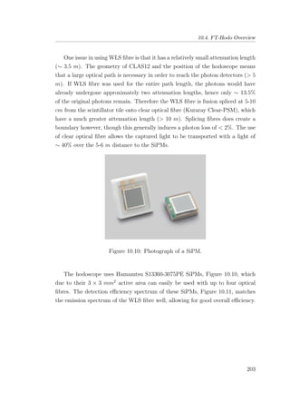
![10.5. FT-Hodo Design
Figure 10.11: Detection efficiency spectrum of the SiPMs [118].
10.5 FT-Hodo Design
The spatial resolution of the hodoscope should be a good match for that of the
FT-Cal. To comply with this the hodoscope used pixels of 15 × 15 mm (P15s),
which covers a single crystal in the FT-Cal and pixels of 30 × 30 mm (P30s)
which cover four crystals of the FT-Cal. These sizes were chosen to compromise
between minimising the number of tile boundaries and maximising the number
of photons which can be collected by the WLS fibre. The arrangement of these
detector elements which make up a layer of the hodoscope is shown in Figure
10.12.
204](https://image.slidesharecdn.com/6d482e98-273b-437a-88cf-eb4faf084ce1-161109162450/85/thesis-231-320.jpg)
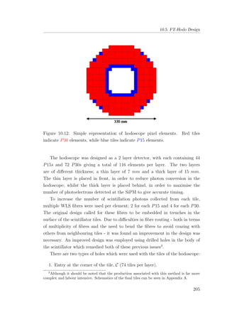
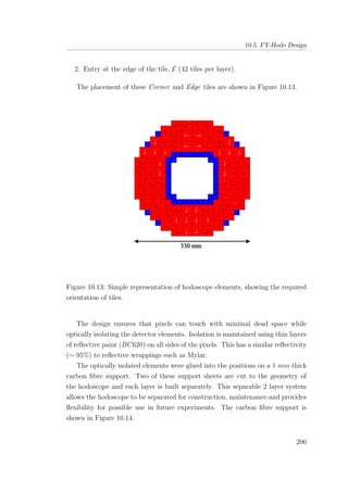
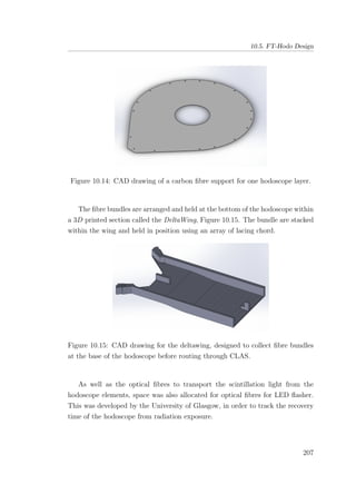
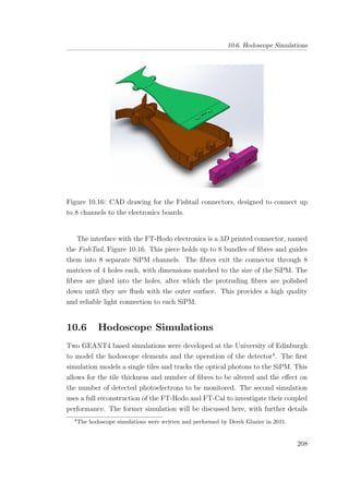
![10.6. Hodoscope Simulations
available for these simulations available in [114].
The validity of the simulation was checked for by comparing consistency to
the CLAS Inner Calorimeter hodoscope. The set-up from this detector yielded
18 photoelectrons per MIP, which was in agreement with the most likely value of
the simulated set-up, shown in Figure 10.17.
Figure 10.17: Number of photons detected for tile geometry similar to the
previous CLAS Inner Calorimeter, which measured 18 photons per MIP [114].
The simulation used the GEANT4 framework, with energy deposits handled
using the standard physics classes available. The optical light produced was
modelled with the parameters of the construction materials used (light output,
reflectivity, etc.) The simulation was then used to explore possible tile and fibre
designs for the hodoscope.
A common feature of all the simulations carried out are that they are trialled
with multiple fibre-options per tile, typically 1 fibre, 2 fibres and 4 fibres.
10.6.1 Tile Thickness Simulations
The number of photons detected were considered while varying number of fibres,
as well as timing resolution. Figure 10.18 shows the number of photons detected
for P15 and P30 elements. This details the photons while the tile thickness is
increased and the number of fibres per tile is also varied.
209](https://image.slidesharecdn.com/6d482e98-273b-437a-88cf-eb4faf084ce1-161109162450/85/thesis-236-320.jpg)
![10.6. Hodoscope Simulations
Figure 10.18: The number of photons detected for different configurations of tile.
Left: P15. Right: P30 [114].
The simulation illustrates important effects in tile thickness and fibre number.
Comparing P15 and P30 elements we see that the increase in size alters the
detected photons by more than a factor of 2. While doubling the number of
fibres gives less than a factor of 2 increase in the number of detected photons.
Simulation results for the tiles used in the final construction are shown in Table
10.3, where P15s are read out by two fibres and P30s are read out by four fibres.
Tile Size Tile Thickness(mm) Approx. Number of Photons
P15 7 70
15 150
P30 7 55
15 120
Table 10.2: Summary of approximate numbers of photons expected for tiles
similar to those used in the final hodoscope construction.
10.6.2 Timing Resolution
The results for the timing resolution simulation are given in Figure 10.19.
210](https://image.slidesharecdn.com/6d482e98-273b-437a-88cf-eb4faf084ce1-161109162450/85/thesis-237-320.jpg)
![10.6. Hodoscope Simulations
Figure 10.19: Timing resolution for different configurations of tile. Left: P15.
Right: P30 [114].
The key point to notice here is that to improve the timing resolution it is
important to maximise the number of detected photons. The simulation indicates
that sub nanosecond timing resolution is attainable for the kinds of configurations
that were used. Simulation results for the tile timing resolution used in the final
construction are shown in Table 10.3.
Tile Size Tile Thickness (mm) Approx. Timing Resolution (ns)
P15 7 0.40
15 0.30
P30 7 0.50
15 0.35
Table 10.3: Summary of approximate timing resolution expected for tiles similar
to those used in the final hodoscope construction.
10.6.3 Fibre Bending
Fibre bending was the last effect which was considered in order to study light
loss due to routing in CLAS and within the hodoscope enclosure itself. Figure
211](https://image.slidesharecdn.com/6d482e98-273b-437a-88cf-eb4faf084ce1-161109162450/85/thesis-238-320.jpg)
![10.6. Hodoscope Simulations
10.20 was generated in order to show the amount of light lost from the fibre as a
function of the bending radius.
Figure 10.20: Effect of bending a fibre. Shown is the fraction of photons
transmitted to the detector as a function of the bend radius of the fibre [114].
10.6.4 Radiation Dose
Simulations for the radiation exposure of the hodoscope and calorimeter were
carried out by INFN Genoa. These were important, in order to assess the exposed
dose and to ensure this wouldn’t lead to significant degradation of the hodoscope’s
efficiency during running.
The simulations showed that the rate on the innermost pixels was equal to
3.8 rad/h without the Møller shield in place. A plot from the INFN simulation
is shown in Figure 10.21.
212](https://image.slidesharecdn.com/6d482e98-273b-437a-88cf-eb4faf084ce1-161109162450/85/thesis-239-320.jpg)
![10.6. Hodoscope Simulations
Figure 10.21: Radiation dose on the FT calorimeter crystals in rad/hour at 1035
cm−2
s−1
luminosity. The maximum values of about 5 rad/h are observed for the
innermost crystals [114].
Since 3.8 rad/h is the highest rate, we assumed this to be the rate over the
entire hodoscope, rather than just the innermost pixels. This gives a yearly rate
of 33 krad. It is known that the irradiation of scintillator causes the properties of
the material to change; which leads to a reduction in light yield and a degradation
in energy resolution. Similar effects are seen in wavelength shifting fibre where
transparency, attenuation length and brightness are reduced.
There are many studies outlining the effects of radiation damage on scintil-
lators and wavelength shifting fibre. For example, [119] suggests that doses of
10-100 krad may overcome difficulties of damage and only once the exposure
reaches ∼ 1 Mrad is damage a concern, becoming irreversibly damaged at 10
Mrad. Many other sources, [120] [121] [122], suggest that damage is only a
concern at the Mrad level and even that lower rates (0.64 krad/h) can recover
while being irradiated. It should be noted that the doses in these studies are
given over a period of hours and total dose is of the Mrad level, whereas over a
year our total dose is of the 10 krad level. From this, we conclude that at the
dose rate expected at CLAS12, the hodoscope is sufficiently radiation hard.
213](https://image.slidesharecdn.com/6d482e98-273b-437a-88cf-eb4faf084ce1-161109162450/85/thesis-240-320.jpg)
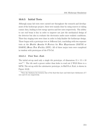
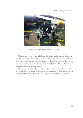
![10.6. Hodoscope Simulations
Figure 10.23: A sample result from the first test at JLab. Shown is the
central calorimeter energy vs the hodoscope energy (presented in terms of ADC
channel). The small left-hand cluster represents a pedestal, while the large right-
hand cluster represents a coincidence measurement between the hodoscope and
calorimeter element.
The initial readout set-up provided positive results but also gave many areas
of development for the project. These included the optical isolation of the tile;
improving the optical connection from fibre to SiPM and considering how this
would work for multiple channels.
10.6.5.2 Second Test: BTF at DAΦNE
DAΦNE is an e−
-e+
collider at the INFN Frascati National Laboratory, Figure
10.24. The LINAC is used to accelerate electrons and positrons to W = 1.02
GeV in order to create φ mesons, which decay into kaons. The BTF [123] is a
beam transfer line which allows users to use the DAΦNE facility as a source of
electrons and positrons for multiplicity or single-electron running modes.
216](https://image.slidesharecdn.com/6d482e98-273b-437a-88cf-eb4faf084ce1-161109162450/85/thesis-243-320.jpg)
![10.6. Hodoscope Simulations
Figure 10.24: Ariel schematic of the DAΦNE complex [123].
The purpose of this second test was to test multiple hodoscope channels in
conjunction with multiple calorimeter channels. A total of 8 tiles were prepared
for this test; 4 P15 elements and 4 P30 which were then split equally between
thin (7 mm) and thick (15 mm) tiles. Similarly to the initial test at JLab, the
tiles were mounted in front of the calorimeter tile. To facilitate ease of readout
the tiles on the left were provided with longer WLS fibre (∼ 1 m) than the right
side (∼ 0.2 m)6
. This set-up is shown in a simple schematic, Figure 10.25.
6
Note that the fibres are glued with UV curing glue and still reading out in channels rather
than holes. Wrapping uses aluminiumised Mylar rather than reflective paint.
217](https://image.slidesharecdn.com/6d482e98-273b-437a-88cf-eb4faf084ce1-161109162450/85/thesis-244-320.jpg)
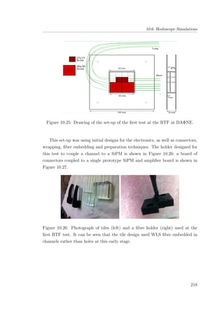
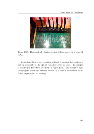
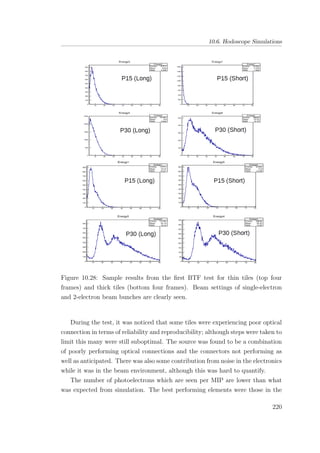
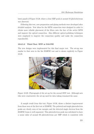
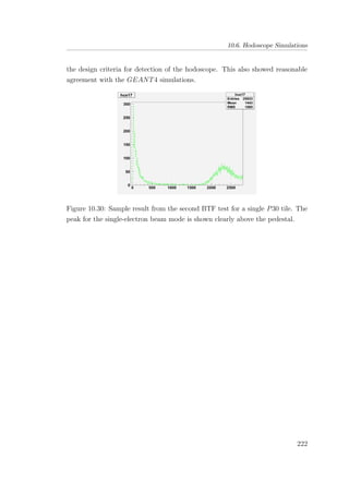
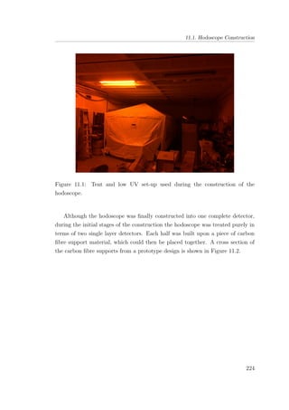
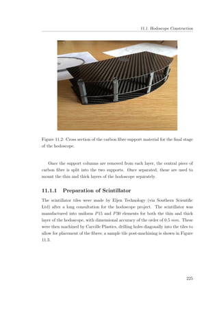
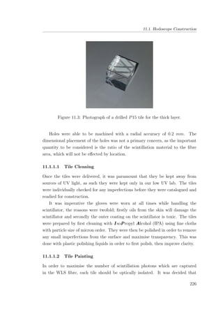
![11.1. Hodoscope Construction
the isolation would be achieved by using reflective paint (specifically BC-622A
Reflector Paint [124]). This was selected after considering factors such as total
reflectivity, application thickness, work hours required and ability to quality
control.
The reflector was applied using fine round, rigger and angle paint brushes2
.
The minimum requirement for paint thickness per side was defined as 0.15 mm;
this and a detailed visual inspection of each tile were the criteria for passing the
first stage of QC. An example of a prepared tile is shown in Figure 11.4.
Figure 11.4: Tile shown post-painting. Dummy fibres and aluminium foil were
used to protect the drilled channels.
It should also be made clear that the addition of paint adds ‘size’ to the tile.
The additional thickness introduced leads to outer tiles of the hodoscope being
displaced by the order of several mms. The assigned 0.15 mm thickness is a
compromise between a highly reflective surface and a minimised movement of the
outer tiles. The concern of this is twofold: firstly, any tiles which exceed the outer
radius of the hodoscope area must be cut and secondly, additional tile thickness
increases dead regions within the detector,
Once the tiles were painted the first round of QC is performed. This is a
visual inspection where any areas which are obviously too thin or streaked must
be repainted, the goal of this is to obtain as close to a smooth homogeneous finish
as possible. It was necessary to have a thickness larger than 0.15 mm and then to
2
This was done in shifts by several members of the department, some of whom were actively
involved in the hodoscope project and others who were not. While the painting was done by
many people, the Quality Control (QC) and additional tile corrections were only undertaken
by myself.
227](https://image.slidesharecdn.com/6d482e98-273b-437a-88cf-eb4faf084ce1-161109162450/85/thesis-254-320.jpg)
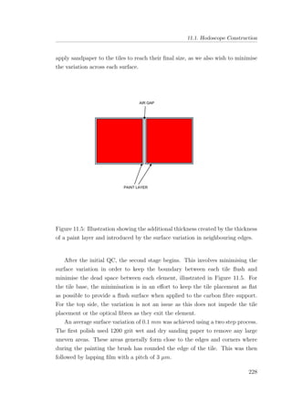
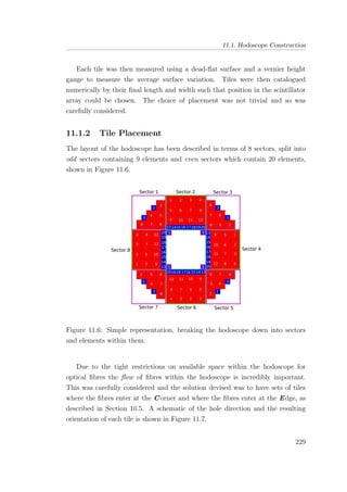
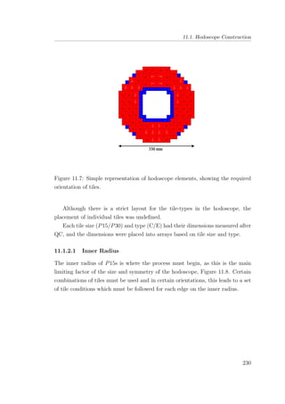
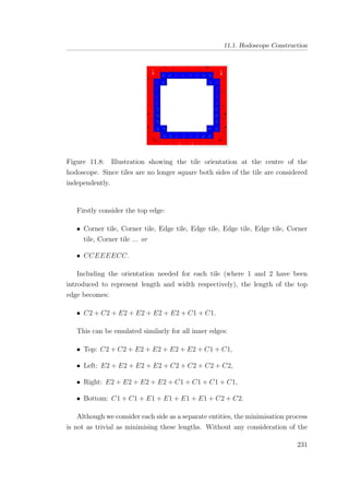
![11.1. Hodoscope Construction
correlation of edges, it is easy to end up with asymmetries and a skewed inner
radius. To overcome this, some further considerations must be made. Along
with the intra-edge properties defined above we also must consider the inter-edge
properties. These include the constructed inner circumference to parametrise the
inner radius, ζ. The relative differences in the intra-edge lengths and the sum
of these values allow for parametrisation of the edge symmetry, ξ. The final
minimisation function, χ, becomes some weighting of these two variables:
χinner = Aζ + Bξ, (11.1)
where A, B ∈ Q[0, 1] and A+B
!
= 1. This allows the importance of minimisation
and symmetry to be carefully balanced and experimented with to find an ideal
configuration.
The minimisation process randomly selects tiles of the appropriate type and
orientation, where each can only be selected once. The function χ is then
minimised according to the weighted values of ζ and ξ. Many trials of this
were run with various weightings in order to find a favoured minimisation. The
key to an effective minimisation is a lower number of iterations but many trials
with a different random seed; this method ensures that false local minima do not
strongly influence the result.
11.1.2.2 Even Sectors
The next key stage is minimising the even sectors, the orientations are shown
in Figure 11.9. These four sectors were considered in terms of rows within each
sector. We can sub-divide each sector into three constituent rows and label tiles
as for the inner radius:
232](https://image.slidesharecdn.com/6d482e98-273b-437a-88cf-eb4faf084ce1-161109162450/85/thesis-259-320.jpg)
![11.1. Hodoscope Construction
Figure 11.9: Illustration showing the orientation of tiles in the even sectors of the
hodoscope. These are considered as three rows.
• Sector 2:
(C2 + C2 + C1 + C1) × 1,
(C2 + E2 + E2 + C1) × 2.
• Sector 4:
(C1 + C1 + C1 + C1) × 2,
(E2 + E2 + C1 + C1) × 1.
• Sector 6:
(E1 + E1 + E1 + E1) × 2,
(C1 + E1 + E1 + C2) × 1.
• Sector 8:
(C2 + C2 + C2 + C2) × 2,
(C2 + C2 + E2 + E2) × 1.
Again the minimisation is not trivial. We consider intra-sector properties,
such as the average row size, row deviation from the average and the sum of the
deviations; giving some indication of the squareness of the sector, µ. Inter-sector
properties are also considered, such as the sector deviations from the average
size; giving some indication of the sector symmetry, ν. A new χ function can be
defined:
χouter = Aµ + Bν, (11.2)
where A, B ∈ Q[0, 1] and A + B
!
= 1. This χ is again minimised for weighted
values of µ and ν, for many iterations until a suitable minimisation is found.
233](https://image.slidesharecdn.com/6d482e98-273b-437a-88cf-eb4faf084ce1-161109162450/85/thesis-260-320.jpg)
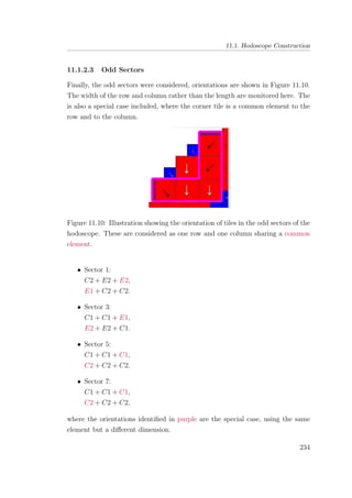
![11.1. Hodoscope Construction
Intra-sector properties are considered such as the average width; the deviation
from the average in a column; the deviation between columns and the sum of
deviations and relative deviations. This gives two considerations: the squareness
of the rows, δ and the symmetry of the rows, λ. Inter-sector properties such as
the deviation from sector averages and sum of these are considered, giving an
insight into the sector symmetry, ψ. We again construct a minimisation function:
χcorner = Aδ + Bλ + Cψ, (11.3)
where A, B, C ∈ Q[0, 1] and A + B + C
!
= 1. This is then minimised with
weightings of A, B and C, in order to find a suitable arrangement.
11.1.2.4 Optimal Tile Arrangement
Each stage of minimisation must be fully completed before continuing onto the
next. This is because once a tile is selected, it must be removed from the array
of available tiles. A fully minimised arrangement in the lab is shown in Figure
11.11.
Figure 11.11: Fully minimised layout for the thick layer of the hodoscope.
Element types are denoted by colour: P30C, P30E, P15C and P15E.
235](https://image.slidesharecdn.com/6d482e98-273b-437a-88cf-eb4faf084ce1-161109162450/85/thesis-262-320.jpg)
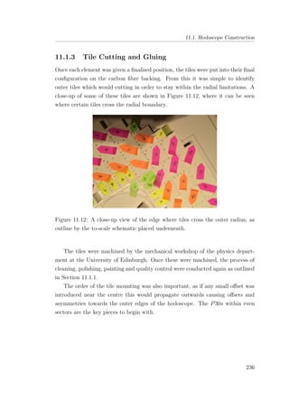
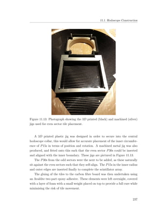
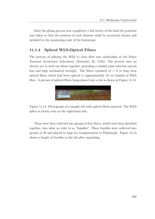
![11.1. Hodoscope Construction
Figure 11.15: Lengths of spliced fibre in the lab.
11.1.4.1 Preparation of Optical Fibres
Each bundle of optical fibre had to be prepared before they could be glued into
the hodoscope elements. This involved similar preparations to that of the tiles,
as outlined in Section 11.1.1.
The fibre ends were polished using sand paper from coarse grain down to 3
µm lapping paper. These were then thoroughly cleaned using IPA, before being
painted with reflective paint in order to maximise the number of photons collected
in the fibres.
Each bundle labelled numerically at both ends, so that each bundle could be
mapped to the corresponding hodoscope elements. It is important to remember
that each bundle consists of four optical fibres. Due to spatial limitations, there
are not sufficient space for each element to have a dedicated bundle. Therefore two
P15 elements were forced to share a bundle. Once the fibre ends were prepared
the gluing process could begin.
11.1.4.2 Optical Fibre Gluing
The optical adhesive chosen for gluing the fibres into the drilled channels of the
tiles was Epotek 301-2 [125], a two part epoxy with very good optical properties
and resistance to radiation damage. Once mixed it was placed in a vacuum
239](https://image.slidesharecdn.com/6d482e98-273b-437a-88cf-eb4faf084ce1-161109162450/85/thesis-266-320.jpg)
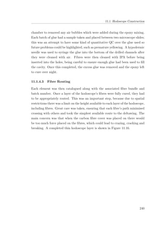
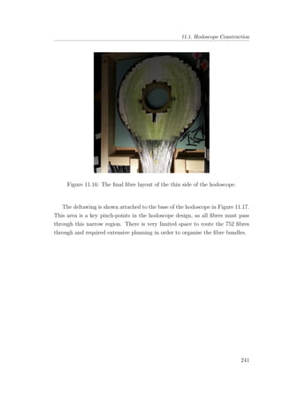
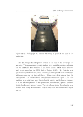
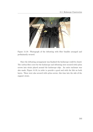
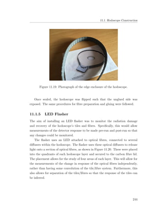
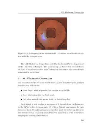
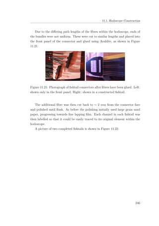
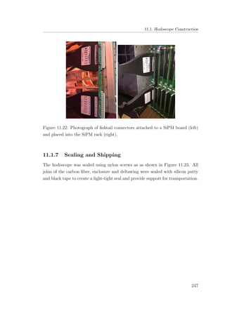
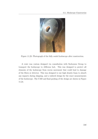
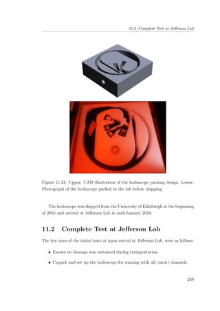
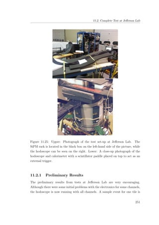
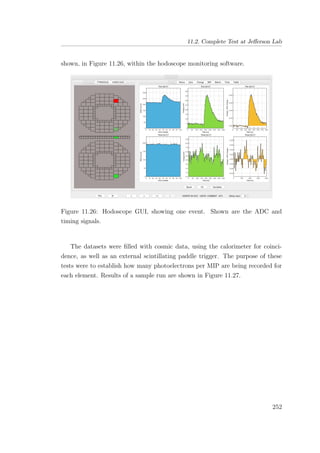
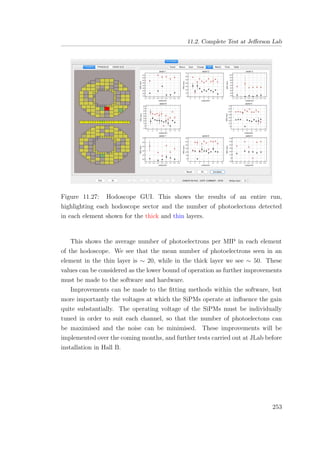
![Bibliography
[1] B.R. Martin and G. Shaw. Particle Physics. Wiley & Sons Ltd, 1999.
[2] D. Griffiths. Introduction to Elementary Particles. Wiley-VCH, Weinheim, 2008.
[3] F.E Close. An Introduction to Quarks and Partons. Academic Press Limited,
London, 1989.
[4] S. Bethke. Experimental Tests of Asymptotic Freedom. Prog. Part. Nucl. Phys.,
58:351–386.
[5] I. Montvay and G M¨unster. Quantum Fields on a Lattice. Cambridge University
Press, 1997.
[6] J. Smit. Introduction to Quantum Fields on a Lattice. Cambridge University
Press, 2002.
[7] Cern Courier. HERMES Searches for the Nucleon’s Missing Spin, Oct 31 2001.
http://cerncourier.com/cws/article/cern/28532/2.
[8] Dr W. Roberts (Florida State University). Meson Nonet, 2006. http://web2.
physics.fsu.edu/~roberts/roberts_quark_model.html.
[9] Dr W. Roberts (Florida State University). Baryon Octet, 2006. http://web2.
physics.fsu.edu/~roberts/roberts_quark_model.html.
[10] K. Nakamura et al. (Particle Data Group). Review of Particle Physics. Journal
of Physics G, 37:075021.
[11] M. Battaglieri et al. Meson Spectroscopy with Low Q2 Electron Scattering in
CLAS12. Proposal to PAC37, V2.3, 2010.
[12] J. Messchendorp for the BESIII Collaboration. Physics with Charmonium – A
few recent highlights of BESIII, PoS Bormio2013 2013. Conference: C13-01-21.2
Proceedings.
[13] S. Niccolai. The Physics Program of CLAS12. Nucl. Phys. B, 210-211:119–124,
2011.
[14] E.S. Smith. The 12GeV JLab Upgrade Project. Nucl. Phys. A, 827:599c–604c,
2009.
256](https://image.slidesharecdn.com/6d482e98-273b-437a-88cf-eb4faf084ce1-161109162450/85/thesis-283-320.jpg)
![BIBLIOGRAPHY
[15] I. Nakamura. Radiation Damage of Pixelated Photon Detector by Neutron
Radiation. Nucl. Inst. Meth. A, 610:110–113, 2009.
[16] R.L. Jaffe et al. Unconventional States of Confined Quarks and Gluons. Phys.
Lett., B60:201, 1976.
[17] D. Horn and J Mandula. Models of Mesons with Constituent Gluons. Phys. Rev.
D, 17:898, 1978.
[18] T. Barnes et al. q¯qg Hermaphrodite Mesons in the MIT Bag Model. Nucl. Phys.
B, 224:241, 1983.
[19] P. Guo et al. Heavy Quarkonium Hybrids from Coulomb Gauge QCD. Phys.
Rev. D, 78:056003, 2008.
[20] N. Isgur et al. Gluonic Excitations of Mesons: Why they are missing and where
to find them. Phys. Rev. Lett., 54:869, 1985.
[21] N. Isgur et al. Flux-tube Model for Hadrons in QCD. Phys. Rev. D, 31:2910,
1985.
[22] J.J. Dudek et al. Highly Excited and Exotic Meson Spectrum from Dynamical
Lattice QCD. Phys. Rev. Lett., 103:262001, 2009.
[23] J.J. Dudek et al. Toward the Excited Meson Spectrum of Dynamical QCD. Phys.
Rev. D, 82:034508, 2010.
[24] D.I. Glazier (on behalf of the CLAS collaboration). A Quasi-real Photon Tagger
for CLAS12. Nucl. Phys. B, 207-208:204–207, 2010.
[25] E. Klempt and J.M. Richard. Baryon Spectroscopy. Rev. Mod. Phys., 82, 2010.
[26] T. DeGrand et al. Masses and Other Parameters of the Light Hadrons. Phys.
Rev. D, 12:2060, 1975.
[27] D. Diakonov. Foundations of the Constituent Quark Model. Lecture at the
International School of Nuclear Physics, 1995. arXiv:nucl-th/9603023v1.
[28] S. Capstick and W. Roberts. Strange Decays of Nonstrange Baryons. Phys. Rev.
D, 58:074011, 1998.
[29] M. Anselmino et al. Diquarks. Rev. Mod. Phys., 65:1199, 1993.
[30] Crystal Barrel. Baryon Spectroscopy. https://www1.cb.uni-bonn.de/index.
php?id=3.
[31] E. Santopinto and J. Ferretti. Strange and Non-strange Baryon Spectra in
the Relativistic Interacting Quark-Diquark Model with a G¨ursey and Radicati-
inspired Exchange Interaction. Phys. Rev. C, 92:025202, 2015.
[32] M. Hess et al. Diquark Masses from Lattice QCD. Phys. Rev. D, 58:111502, 1998.
257](https://image.slidesharecdn.com/6d482e98-273b-437a-88cf-eb4faf084ce1-161109162450/85/thesis-284-320.jpg)
![BIBLIOGRAPHY
[33] T. DeGrand et al. Diquark Effects in Light Baryon Corrrelators from Lattice
QCD. Phys. Rev. D, 77:034505, 2008.
[34] P. Hasenfratz and J. Kuti. The Quark Bag Model. Phyiscs Reports, 40 - 2:75–179,
1978.
[35] A.W. Thomas et al. Cloudy Bag Model of the Nucleon. Phys. Rev. D, 24:216,
1981.
[36] R.C. Giles et al. Semiclassical Dynamics of the “SLAC Bag”. Phys. Rev. D,
13:1670, 1976.
[37] Hiroshima University. Theoretical Particle Physics. http:
//core-u.hiroshima-u.ac.jp/en/research-groups-en/
theoretical-particle-physics-en.html.
[38] A.V. Anisovich et al. The Impact of New Polarization Data from Bonn, Mainz and
Jefferson Laboratory on γp → πN Multipoles. 2016. arXiv:nucl-th/1604.05704v1.
[39] V.D. Burkert. Meson Production and Baryon Resonances at CLAS. International
Journal of Modern Physics A, 3/4:493–498, 2011.
[40] S. D¨urr. Ab Initio Determination of Light Hadron Masses. Science, 322:1224,
2008.
[41] J.J. Dudek et al. Toward the Excited Isoscalar Meson Spectrum from Lattice
QCD. Phys. Rev. D, 88:094505, 2013.
[42] J.J. Dudek et al. Excited State Baryon Spectroscopy from Lattice QCD. Phys.
Rev. D, 84:074508, 2011.
[43] V.D. Burkert. Nulceon Resonance Physics. 2016. arXiv:nucl-ex/1603.00919.
[44] T. Sato. Osaka University, August 2014. http://research.
dsu.edu/cetup/documents/2014-talks/neutrino-interactions/
Electroweak-Meson-Production(Toru-Sato).pdf.
[45] R. Shankar. Principles of Quantum Mechanics. Springer, 1994.
[46] G.F. Chew et al. Relativistic Dispersion Relation Approach to Photomeson
Production. Phys. Rev., 106:1345, 1957.
[47] I.S. Barker and A. Donnachie. Complete Experiments in Pseudoscalar
Photoproduction. Nucl. Phys. B, 95:347–356, 1975.
[48] R.A. Adelseck and B. Saghai. Kaon Photoproduction: Data Consistency,
Coupling Constants, and Polarization Observables. Phys. Rev. C, 42:108–127,
1990.
[49] W. Chiang and F. Tabakin. Completeness Rules for Spin Observables in
Pseudoscalar Meson Photoproduction. Phys. Rev. C, 55:2054, 1997.
258](https://image.slidesharecdn.com/6d482e98-273b-437a-88cf-eb4faf084ce1-161109162450/85/thesis-285-320.jpg)
![BIBLIOGRAPHY
[50] A.M. Sandorfi et al. Determining Pseudoscalar Meson Photo-production
Amplitudes from Complete Experiments. 2011. arXiv:nucl-th/1010.4555v2.
[51] F.X. Lee et al. Quasifree Kaon Photoproduction on Nuclei. Nucl. Phys. A,
695:237, 2001.
[52] X. Cao. Disentangling the Nature of Resonances in Coupled-channel Models.
Chinese Phys. C, 39:041002, 2015.
[53] Andrey Sarantsev. Properties of Baryons from Bonn-Gatchina Partial Wave
Analysis. JPS Conf. Proc., 10:010005, 2016.
[54] E. Munevar. Photon Beam Asymmetry Measurement from the γn → K+Σ−
Reaction. PhD thesis, George Washington University, 2014.
[55] R.L. Anderson et al. Photoproduction of K+ Mesons from Deuterium. Phys.
Rev., 123:1003, 1961.
[56] B.D. McDaniel et al. Photoproduction of K+ Mesons. Phys. Rev., 115:1039,
1959.
[57] R.L. Anderson et al. Photoproduction of K+ Mesons in Hydrogen. Conference
Proceedings of Annual Conference of High Energy Physics, 1960.
[58] H. Kohri et al. Differential Cross Section and Photon-Beam Asymmetry for the
γn → K+Σ− Reaction at Eγ 1.5 − 2.4 GeV . Phys. Rev. Lett., 97:082003, 2006.
[59] P.D.B. Collins. An Introduction to Regge Theory and High Energy Physics.
Cambridge University Press, 2011.
[60] S.A Pereira et al. Differential Cross Section of γn → K+Σ− on Bound Neutrons
with Incident Photons from 1.1 − 3.6 GeV . Phys. Lett. B, 688:289–293, 2010.
[61] F. Klein et al. N Resonances in Pseudo-scalar Meson Photo-production from
Polarized Neutrons in HD and a Complete Determination of the γn → K◦Λ
amplitude. HDice Proposal, 2010.
[62] Jefferson Lab. CEBAF Celebrates Seven Years of Physics, 2012. http://wwwold.
jlab.org/news/articles/2003/cebaf_caption.html.
[63] Jefferson Lab. JLab Picture Exchange. http://www1.jlab.org/ul/jpix.
[64] C.W. Leemann et al. The Continuous Electron Beam Accelerator Facility:
CEBAF at the Jefferson Laboratory. Annu. Rev. Nucl. Part. Sci., 51:413–450,
2001.
[65] S. Fegan. Polarisation Observables from Strangeness Photoproduction on a Frozen
Spin Target with CLAS at Jefferson Lab. PhD thesis, University of Glasgow, 2011.
[66] J. Alcorn et al. Basic Instrumentation for Hall A at Jefferson Lab. Nucl. Inst.
Meth. A, 522:294–346, 2004.
259](https://image.slidesharecdn.com/6d482e98-273b-437a-88cf-eb4faf084ce1-161109162450/85/thesis-286-320.jpg)
![BIBLIOGRAPHY
[67] B.A. Mecking et al. The CEBAF Large Acceptance Spectrometer. Nucl. Inst.
Meth. A, 503:513, 2003.
[68] M. Hauger et al. A High Precision Polarimeter. Nucl. Inst. Meth. A, 462:382,
2001.
[69] Y. Qiang. Detector Development for Jefferson Lab’s 12 GeV Upgrade. Nucl.
Inst. Meth. B, 350:71–76, 2015.
[70] D.I. Sober et al. The Bremsstrahlung Tagged Photon Beam in Hall B at JLab.
Nucl. Inst. Meth. A, 440:263–284, 2000.
[71] Study Blue. https://www.studyblue.com/notes/note/n/
chapter-1-x-ray-production/deck/10725781.
[72] H. ¨Uberall. High-Energy Interference Effect of Bremsstrahlung and Pair
Production in Crystals. Phys. Rev., 103:1055, 1956.
[73] U. Timm. Coherent Bremsstrahlung of Electrons in Crystals. Fortsch. Phys.,
17:765–808, 1969.
[74] K. Livingston. The Stonehenge Technique: A Method for Aligning Coherent
Bremsstrahlung Radiators. Nucl. Inst. Meth. A, 603:205–219, 2009.
[75] H. Olsen and L.C. Maximon. Photon and Electron Polarization in High-Energy
Bremsstrahlung and Pair Production with Screening. Phys. Rev., 114:887, 1959.
[76] I. Zonta. Polarization Observables from 2−pion and ρ Meson Photoproduction
on Polarized HD target at JLab. PhD thesis, Universita Delgi Studi di Roma,
2014.
[77] W. Gohn et al. Beam-spin Asymmetries from Semi-inclusive Pion Electoproduc-
tion. Phys. Rev. D, 89:072011, 2014.
[78] G. Adams et al. The CLAS Cherenkov Detector. Nucl. Inst. Meth. A, 465:414,
2001.
[79] M. Amarian et al. The CLAS Forward Electromagnetic Calorimeter. Nucl. Inst.
Meth. A, 460:239, 2001.
[80] A.J. Street et al. Final Site Assembly and Testing of the Superconducting Toroidal
Magnet for the CEBAF Large Acceptance Spectrometer (CLAS). IEEE Trans.
Mag., 32:2074, 1996.
[81] J. O’Meara et al. A Superconducting Toroidal Magnet for the CEBAF Large
Acceptance Spectrometer. IEEE Trans. Mag., 25:1902, 1989.
[82] Y.G. Sharabian et al. A New Highly Segmented Start Counter for the CLAS
Detector. Nucl. Inst. Meth. A, 556:246–258, 2006.
[83] M.D. Mestayer et al. The CLAS Drift Chamber System. Nucl. Inst. Meth. A,
449:81, 2000.
260](https://image.slidesharecdn.com/6d482e98-273b-437a-88cf-eb4faf084ce1-161109162450/85/thesis-287-320.jpg)
![BIBLIOGRAPHY
[84] F.J. Barbosa et al. A Drift Chamber System for a Toroidal Detector. Nucl. Inst.
Meth. A, 323:19, 1992.
[85] E.S. Smith et al. The Time-of-flight System for CLAS. Nucl. Inst. Meth. A,
432:265, 1999.
[86] G. Rouille et al. A Polarized HD Target Factory in Europe. Nucl. Inst. Meth. A,
464:428–432, 2001.
[87] V. Laine. Polarimetry of the Polarized Hydrogen Deuteride HDice Target Under
an Electron Beam. PhD thesis, Universite Blaise Pascal, 2013.
[88] W.N Hardy and J.R. Graines. Nuclear Spin Relaxation in Solid HD with H2
Impurity. Phys. Rev. Lett, 17:1278, 1966.
[89] D.J. Gardiner and P.R. Graves. Practical Ramen Spectroscopy. Springer Berlin
Heidelberg, 1989.
[90] C. Kittel. Introduction to Solid State Physics. John Wiley and Sons Ltd, 2013.
[91] A. Sandorfi. The g14 HDice Experiment in Hall B, JLab User Meeting
2012. https://www.jlab.org/conferences/ugm/2012/Tuesday/Sandorfi%
20-JLab%20Users%20mtg%20Jun5-12.pdf.
[92] A. Honig et al. New Investigations of Polarized Solid HD Targets. Nucl. Inst.
Meth. A, 356:39–46, 1995.
[93] C.D. Bass et al. A Portable Cryostat for the Cold Transfer of Polarized Solid HD
Targets. Nucl. Inst. Meth. A, 737:107–116, 2014.
[94] C.S. Whisnant et al. HD Gas Purification for Polarized HDice Target Production
at Jefferson Lab. Proceedings of Science, 017, 2009.
[95] D.H. Ho. Measurement of the E Polarisation Observable for γd → π−p(ps),
γd → K0Λ(ps), and γd → π+π−d(0) using CLAS g14 Data at Jefferson Lab.
PhD thesis, Carnegie Mellon University, 2015.
[96] V. Blobel. The BOS System for CLAS Detector. Institut f¨ur Experimental
Physik, Universit¨at Hamburg, 1995.
[97] CERN. ROOT a Data Analysis Framework. https://root.cern.ch/.
[98] K. Livingston. RootBeer. http://nuclear.gla.ac.uk/~kl/rootbeer/manual/
html/rootbeer.php.
[99] E. Pasyuk. A Brief User Guide to GPID, CLAS NOTE 2007-008.
[100] S. Brandt. Statistical and Compuattional Methods in Data Analysis. North
Holland Publishing Company, 1970.
261](https://image.slidesharecdn.com/6d482e98-273b-437a-88cf-eb4faf084ce1-161109162450/85/thesis-288-320.jpg)
![BIBLIOGRAPHY
[101] M. Williams. Measurement of Differential Cross Sections and Spin Density
Matrix Elements along with a Partial Wave Analysis for γp → pω using CLAS
at Jefferson Lab. PhD thesis, Carnegie Mellon University, 2007.
[102] E. Pasyuk. Energy Loss Corrections for Charged Particles in CLAS, CLAS
Internal Report: CLAS-Note 2007-016 2007.
[103] S. Strauch et al. First Measurement of the Polarization Observable E in the
p(γ, π+)n Reaction up to 2.25 GeV . Phys. Lett. B, 750:53, 2015.
[104] Institut f¨ur Kernphysik. An effective Lagrangian Model for Kaon Photo- and
Electroproduction on the Nucleon. http://portal.kph.uni-mainz.de/MAID/
/kaon/.
[105] D. Ho et al. E Asymmetry for γn → π−p from g14 (HDice) Data, CLAS Analysis
Note 2016. Currently in review.
[106] R. De Vita. Meson Spectroscopy at CLAS and CLAS12: the Present and the
Future. AIP Conf. Proc., 1354:141–147, 2011.
[107] A. Afanasev and P.R. Page. Photoproduction and Electroproduction of JPC =
1−+ Exotics. Phys. Rev. A, 57:6771, 1998.
[108] A. Szczepaniak and M. Swat. Role of Photoproduction in Exotic Meson Searches.
Phys. Lett. B, 516:72, 2001.
[109] E.S. Ageev et al. Gluon Polarization in the Nucleon from Quasi-real
Photoproduction of High-p(T) Hadron Pairs. Phys. Lett. B, 633, 2005.
[110] M. Atkinson et al. Photoproduction of φ Mesons by Linearly Polarized Photons
of Energy 20-40 GeV and Further Evidence for a Photoproduced High-Mass KK
Enhancement . Z. Phys. C, 27:233, 1985.
[111] S. Chekanov et al. Measurement of the PhotonProton Total Cross Section at a
Center-of-mass Energy of 209 GeV at HERA. Nucl. Phys. B, 627:3, 2002.
[112] K. Hicks et al. Search for Scalar Mesons at low Q2 using CLAS12. Proposal to
PAC37, V1.0, 2010.
[113] V.D. Burkert. CLAS12 and its Science Program at the Jefferson Lab Upgrade.
2008. arXiv:hep-ph/0810.4718v2.
[114] The CLAS12 Collaboration. CLAS12 Forward Tagger (FT) Technical Design
Report. Technical Report V1.2, Jefferson Laboratory, Newport News, VA,
November 2011.
[115] Southern Scientific. EJ204 Data Sheet. http://www.southernscientific.co.
uk/store/public/application/file/document/EJ204%20data%20sheet.pdf.
[116] Kuraray. Wavelength Shifting Fibers. http://kuraraypsf.jp/psf/ws.html.
262](https://image.slidesharecdn.com/6d482e98-273b-437a-88cf-eb4faf084ce1-161109162450/85/thesis-289-320.jpg)
![BIBLIOGRAPHY
[117] S. Stepanyan et al. Scintillation Hodoscope Reconstruction Software Package and
Calibration Procedures, CLAS NOTE 2009-019.
[118] Hamamatsu. MPPC Data Sheets. http://www.hamamatsu.com/resources/
pdf/ssd/s13360_series_kapd1052e.pdf.
[119] CERN. Review of Radiation Damage Studies on Scintillating Materials used in
HEP Experiments. TIS Commision Report, 1987.
[120] S. Barsuk et al. Radiation Damage of LHCb Electromagnetic Calorimeter.
Submitted to NIM, ITEP, Moscow.
[121] S.W. Han et al. Radiation Hardness Tests of Scintillating Tile/WLS Fibre
Calorimeter Modules. Nucl. Inst. Meth. A, 365:337–351, 1995.
[122] M.M. Hamada et al. Radiation Damage Studies on the Optical and Mechanical
Properties of Plastic Scintillators. Nucl. Inst. Meth. A, 422:148–154, 1999.
[123] G. Mazzitelli et al. DAΦNE Beam Test Facility Comissioning. Proceedings of the
2003 Particle Accelerator Conference.
[124] Saint Gobain. BC-620 Reflector Paint for Plastic Scintillators. http://www.
crystals.saint-gobain.com/uploadedFiles/SG-Crystals/Documents/.
[125] Epoxy Technology. Epo-Tek 301-2 Data Sheet. http://www.epotek.com/site/
administrator/components/com_products/assets/files/Style_Uploads/
301-2.
263](https://image.slidesharecdn.com/6d482e98-273b-437a-88cf-eb4faf084ce1-161109162450/85/thesis-290-320.jpg)