THESIS.DI.AJP.GM

CODING TECHNIQUES FOR
MULTI-USER PHYSICAL-LAYER SECURITY
A Dissertation
Presented to
The Academic Faculty
By
Alexandre J. Pierrot
In Partial Fulfillment
of the Requirements for the Degree
Doctor of Philosophy
in
Electrical and Computer Engineering
School of Electrical and Computer Engineering
Georgia Institute of Technology
August 2015
Copyright © 2015 by Alexandre J. Pierrot

CODING TECHNIQUES FOR
MULTI-USER PHYSICAL-LAYER SECURITY
Defense Examination Committee:
Dr. Matthieu R. Bloch, Advisor
Associate Professor,
Dr. John R. Barry
Professor,
Dr. Steven W. McLaughlin
Professor and Steve W. Chaddick School Chair,
Dr. Mary Ann Weitnauer
Professor,
Dr. Éric Feron
Dutton/Ducoffe Professor,
School of Aerospace Software Engineering

This thesis is dedicated to the memory of my grandfather
Louis Bœuf (1936–2006)

ACKNOWLEDGMENT
I truly owe this thesis to my beloved family, who provided with its love and support for
the last 26 years. My mom, Sandrine, who taught me her sense of esthetics and details,
my dad, Guillaume, who triggered my engineer curiosity, my grandmother, Paulette, who
surrounded me with love and pride, my grandparents, Martine and Jean-Marie, who made
me a citizen of the world, and finally my late grandfather, Louis, who asked me to design
a rocket when I was 5, are the true authors of this work. I am confident that my dear
youngest siblings, Maëva and Enzo, will benefit from the same love and will achieve even
more.
I also found the force to go through these last five years thanks to my forever friends
Alexandra, Isabelle, and Maxime, who have been constantly here for me. I will always
remember that they have traveled for 14 hours to attend my proposal without hesitation.
Together we have accumulated 40 years of study in Law, Medicine, and Engineering, af-
ter going to the same local high school in Marseille, supporting each other in this long
adventure.
In France, Pierre-Alexandre, Manas, and Guillaume have been the best Ph.D. accom-
plices I could have had to clear the gray sky of Metz. Almost two years ago, Atlanta
welcomed me like an old friend thanks to Romain and Andrew, Aude and Manu, Flo,
Tim, and all the other AE folks. Atlanta also brought Kevin into my life, who has been
an amazingly supportive partner to run the last miles, and hopefully the upcoming ones.
Last but not least, there is my advisor Matthieu, or should I say my friend Matthieu,
who supported me far beyond being a simple professor: as a student, I was lucky to have
found a devoted and passionate professor; as a person, I was lucky to have found an
invaluable support. I am proud to be his first student and wish him the best for the next
lucky ones working with him.
iv

REMERCIEMENTS
Je dois, en réalité cette thèse à ma famille chérie, qui m’a donné tout son amour et son
soutient lors de ces 26 dernières années. Les véritables auteurs de cette thèse sont ma mère,
Sandrine, qui m’a enseigné son sens de l’esthétique et du détail, mon père, Guillaume, qui
a su stimuler ma curiosité d’ingénieur, ma grand-mère, Paulette, qui m’a entouré de son
amour et de sa fierté, mes grands parents, Martine et Jean-Marie, qui ont fait de moi un
véritable citoyen du monde, et enfin, feu mon grand-père, Louis, qui m’a demandé de lui
concevoir une fusée quand j’avais cinq ans. Je sais que mes plus jeunes frère et sœur adorés,
Maëva et Enzo, bénéficieront du même amour et en feront encore bien plus.
J’ai aussi trouvé la force de traverser toutes ces années grâce à mes amis d’enfance,
Alexandra, Isabelle et Maxime qui ont été là pour moi à chaque instant. Je me rappellerai
toujours qu’ils ont voyagé 14 heures pour venir à mon proposal sans se poser la moindre
question. Ensemble, nous avons cumulé plus de 40 ans d’études en Droit, Médecine et
Ingénierie, se soutenant les uns les autres dans cette longue aventure.
En France, Pierre-Alexandre, Manas et Guillaume ont été les meilleurs comparses de
doctorat que j’aurais pu avoir pour éclaircir le ciel gris de Metz. Il y a quasiment deux ans,
Atlanta m’a accueilli comme un vieil ami grâce à Romain et Andrew, Aude et Manu, Flo,
Tim et tous les autres de l’école de Génie Aérospatial. Atlanta a aussi apporté dans ma vie
Kevin, qui a été un partenaire merveilleux durant ces dernières années, et je l’espère pour
celles à venir.
Enfin, et pas des moindres, il y a mon directeur de thèse, Matthieu, ou devrais-je dire
mon ami, Matthieu, qui m’a soutenu bien au delà de son rôle de professeur. En tant
qu’étudiant, j’ai eu l’opportunité de travailler avec un professeur dévoué et passionné. En
tant que personne, j’ai eu la chance de trouver un soutient indéfectible. Je suis fier d’être
son premier étudiant et je lui souhaite le meilleur pour ceux à venir.
v

CONTENTS
ACKNOWLEDGMENT . . . . . . . . . . . . . . . . . . . . . . . . . . . . . . iv
LIST OF TABLES . . . . . . . . . . . . . . . . . . . . . . . . . . . . . . . . . . ix
LIST OF FIGURES . . . . . . . . . . . . . . . . . . . . . . . . . . . . . . . . . xi
CHAPTER 1 INTRODUCTION . . . . . . . . . . . . . . . . . . . . . . . . 1
1.1 From Mathematical Cryptography to Physical-Layer Security . . . . . . 3
1.2 Information-Theoretic Security: the Wiretap Channel . . . . . . . . . . 4
1.3 Multi-User Information-Theoretic Security . . . . . . . . . . . . . . . . 7
1.3.1 Cooperative Jamming and Coded cooperative jamming . . . . 8
1.3.2 Key Exchange . . . . . . . . . . . . . . . . . . . . . . . . . . . 8
1.3.3 Secret-Key Generation Strategy . . . . . . . . . . . . . . . . . 9
1.4 Experimental Aspects . . . . . . . . . . . . . . . . . . . . . . . . . . . 10
1.5 Contributions . . . . . . . . . . . . . . . . . . . . . . . . . . . . . . . 10
CHAPTER 2 INFORMATION-THEORETIC SECURITY . . . . . . . . . . 13
2.1 Tools of Information Theory . . . . . . . . . . . . . . . . . . . . . . . 13
2.1.1 Entropy and Mutual Information . . . . . . . . . . . . . . . . 13
2.1.2 Rényi Entropy . . . . . . . . . . . . . . . . . . . . . . . . . . 18
2.1.3 Other Metrics . . . . . . . . . . . . . . . . . . . . . . . . . . 19
2.1.4 Typical Sequences . . . . . . . . . . . . . . . . . . . . . . . . 21
2.1.5 Markov Chains and Functional Dependence Graphs . . . . . . 26
2.1.6 Information-Theoretic Bounds . . . . . . . . . . . . . . . . . . 27
2.2 Coding Primitives . . . . . . . . . . . . . . . . . . . . . . . . . . . . . 28
2.2.1 Channel Capacity . . . . . . . . . . . . . . . . . . . . . . . . 28
2.2.2 Source Coding with Side Information . . . . . . . . . . . . . . 30
2.2.3 Channel Intrinsic Randomness . . . . . . . . . . . . . . . . . . 34
2.2.4 Channel Resolvability . . . . . . . . . . . . . . . . . . . . . . 35
2.3 Joint Analysis of Channel Intrinsic Randomness and Resolvability . . . 36
2.3.1 Definitions and Assumptions . . . . . . . . . . . . . . . . . . 36
2.3.2 Achievability and Exponents . . . . . . . . . . . . . . . . . . . 38
2.3.3 Converse . . . . . . . . . . . . . . . . . . . . . . . . . . . . . 43
2.3.4 Discussion . . . . . . . . . . . . . . . . . . . . . . . . . . . . 45
CHAPTER 3 THE TWO-WAY WIRETAP CHANNEL . . . . . . . . . . . . 47
3.1 Problem Statement . . . . . . . . . . . . . . . . . . . . . . . . . . . . 48
3.2 Resolvability-Based Cooperative Jamming . . . . . . . . . . . . . . . . 51
3.2.1 Cooperative Jamming . . . . . . . . . . . . . . . . . . . . . . 51
3.2.2 Achievable Region . . . . . . . . . . . . . . . . . . . . . . . . 52
3.3 Secret-Key Exchange and Secret-Key Generation . . . . . . . . . . . . . 58
3.3.1 Key Exchange . . . . . . . . . . . . . . . . . . . . . . . . . . . 58
vi

3.3.2 Key Generation from Induced Source . . . . . . . . . . . . . . 60
3.3.3 Achievable Region with Secret-Key Exchange and Generation . 61
3.4 Gaussian Two-Way Wiretap Channel . . . . . . . . . . . . . . . . . . . 69
3.4.1 Randomness Source Extraction . . . . . . . . . . . . . . . . . 70
3.4.2 Results . . . . . . . . . . . . . . . . . . . . . . . . . . . . . . 72
3.5 Conclusion and Discussion . . . . . . . . . . . . . . . . . . . . . . . . 74
CHAPTER 4 EXPERIMENTAL ASPECTS OF KEY GENERATION . . . . 75
4.1 Key Generation from Channel Variations . . . . . . . . . . . . . . . . 77
4.1.1 Secret-Key Generation Strategy . . . . . . . . . . . . . . . . . 77
4.1.2 Mathematical Formalism . . . . . . . . . . . . . . . . . . . . . 79
4.1.3 Assumptions behind the secret-key generation model . . . . . . 80
4.2 Experimental Source Induction . . . . . . . . . . . . . . . . . . . . . . 81
4.2.1 Setup Description . . . . . . . . . . . . . . . . . . . . . . . . 82
4.2.2 Communication Chain . . . . . . . . . . . . . . . . . . . . . . 82
4.2.3 Characterization of Induced Source Statistics. . . . . . . . . . . 83
4.3 Statistics of the Channel Gain Observations . . . . . . . . . . . . . . . 86
4.3.1 Empirical Gain Distribution . . . . . . . . . . . . . . . . . . . 86
4.3.2 Robustness of the Diversity Assumption . . . . . . . . . . . . . 87
4.3.3 Environment Influence . . . . . . . . . . . . . . . . . . . . . . 90
4.4 Secret-Key Generation in the Finite Blocklength Regime . . . . . . . . 92
4.4.1 Finite-Length Analysis for a Continuous Observation Z . . . . 92
4.4.2 Numerical Evaluation . . . . . . . . . . . . . . . . . . . . . . 95
CHAPTER 5 PRACTICAL CODED COOPERATIVE JAMMING . . . . . 99
5.1 Coded Cooperative Jamming for the Two-Way Wiretap Channel . . . . 100
5.1.1 General Model . . . . . . . . . . . . . . . . . . . . . . . . . . 100
5.1.2 Erasure MAC . . . . . . . . . . . . . . . . . . . . . . . . . . . 101
5.1.3 Leakage Analysis . . . . . . . . . . . . . . . . . . . . . . . . . 102
5.2 LDPC Codes for the MAC . . . . . . . . . . . . . . . . . . . . . . . . 103
5.2.1 Spatially-Coupled LDPC Codes . . . . . . . . . . . . . . . . . 104
5.2.2 Spatially-Coupled LDPC Codes for the MAC . . . . . . . . . . 106
5.3 Punctured LDPC Codes for the MAC . . . . . . . . . . . . . . . . . . 109
5.3.1 Code Construction . . . . . . . . . . . . . . . . . . . . . . . . 109
5.3.2 Leakage Analysis . . . . . . . . . . . . . . . . . . . . . . . . . 110
5.3.3 Reliability Analysis . . . . . . . . . . . . . . . . . . . . . . . . 112
5.3.4 Numerical Results . . . . . . . . . . . . . . . . . . . . . . . . 112
CHAPTER 6 CONCLUSION . . . . . . . . . . . . . . . . . . . . . . . . . . 119
6.1 Contributions . . . . . . . . . . . . . . . . . . . . . . . . . . . . . . . 119
6.2 Perspectives . . . . . . . . . . . . . . . . . . . . . . . . . . . . . . . . 120
vii

CHAPTER 7 APPENDIX . . . . . . . . . . . . . . . . . . . . . . . . . . . . 122
7.1 Coding with Polar Codes . . . . . . . . . . . . . . . . . . . . . . . . . 122
7.2 Universal Software Radio Peripherals (USRPs) . . . . . . . . . . . . . . 123
7.3 Proofs of Lemmas . . . . . . . . . . . . . . . . . . . . . . . . . . . . . 128
7.3.1 Proof of Lemma 3.2 . . . . . . . . . . . . . . . . . . . . . . . 128
7.3.2 Proof of Lemma 3.3 . . . . . . . . . . . . . . . . . . . . . . . 130
7.3.3 Proof of Lemma 3.6 . . . . . . . . . . . . . . . . . . . . . . . 133
7.3.4 Proof of Lemma 3.7 . . . . . . . . . . . . . . . . . . . . . . . 137
7.3.5 Proof of Lemma 4.1 . . . . . . . . . . . . . . . . . . . . . . . 138
VITA . . . . . . . . . . . . . . . . . . . . . . . . . . . . . . . . . . . . . . . . . 152
viii

LIST OF TABLES
Table 3.1 Additional constraints for secret-key generation. . . . . . . . . . . . . 69
Table 4.1 Literature comparison. . . . . . . . . . . . . . . . . . . . . . . . . . . 75
Table 4.2 Gain measurement entropy and secret-key rate upper bound in various
situations. . . . . . . . . . . . . . . . . . . . . . . . . . . . . . . . . 91
Table 5.1 Advantages of spatially coupled LDPC codes. . . . . . . . . . . . . . . 113
Table 7.1 Comparisons of the different USPR models. . . . . . . . . . . . . . . 124
ix

LIST OF FIGURES
Figure 1.1 Communications over the degraded wiretap channel. . . . . . . . . . 5
Figure 1.2 Nested structure of a wiretap code. . . . . . . . . . . . . . . . . . . . 6
Figure 1.3 Capacity versus resolvability. . . . . . . . . . . . . . . . . . . . . . . . 6
Figure 1.4 Simple multi-user scheme with eavesdropper. . . . . . . . . . . . . . . 7
Figure 1.5 Secret-key exchange. . . . . . . . . . . . . . . . . . . . . . . . . . . . 9
Figure 2.1 Functional dependence graph of Example 2.1.5. . . . . . . . . . . . . 26
Figure 2.2 Point-to-point communications. . . . . . . . . . . . . . . . . . . . . 28
Figure 2.3 Binary symmetric channel and binary erasure channel. . . . . . . . . . 29
Figure 2.4 The Slepian-Wolf problem. . . . . . . . . . . . . . . . . . . . . . . . 30
Figure 2.5 The Slepian-Wolf region for a discrete memoryless source (XY,pXY ). . 32
Figure 2.6 Binning procedure for the Slepian-Wolf coding. . . . . . . . . . . . . 33
Figure 2.7 Channel Intrinsic Randomness (CIR) basic scheme. . . . . . . . . . . 34
Figure 2.8 Channel Resolvability basic scheme. . . . . . . . . . . . . . . . . . . . 35
Figure 2.9 Joint channel intrinsic randomness and resolvability. . . . . . . . . . . 37
Figure 2.10 Comparison of joint and tandem exponents. . . . . . . . . . . . . . . 40
Figure 2.11 Determining the tandem exponent. . . . . . . . . . . . . . . . . . . . 43
Figure 3.1 Communication over a two-way wiretap channel. . . . . . . . . . . . 49
Figure 3.2 Communication over a two-way wiretap channel without feedback. . . 52
Figure 3.3 Constraints on R′
1 and R′
2 in (3.2). . . . . . . . . . . . . . . . . . . . . 57
Figure 3.4 Dependence graph for with secret-key generation. . . . . . . . . . . . 66
Figure 3.5 Region evaluation for д1 = д2 = 1, ρ1 = 1, ρ2 = 100, h1 = 1, h2 = 0.1. . 72
Figure 3.6 Region evaluation for д1 = д2 = 1, ρ1 = ρ2 = 1, h1 = h2 = 1.5. . . . . . 73
Figure 3.7 Region evaluation for ρ1 = ρ2 = 0.9, h1 = h2 = 10, д1 = д2 = 1. . . . . . 74
Figure 4.1 Experimental testbed with software-defined radios. . . . . . . . . . . . 78
xi

Figure 4.2 Communication chain for channel gain estimation. . . . . . . . . . . 83
Figure 4.3 Channel gain measurements. . . . . . . . . . . . . . . . . . . . . . . 84
Figure 4.4 Evolution of the self-correlation of channel gains. . . . . . . . . . . . 85
Figure 4.5 Gain distribution . . . . . . . . . . . . . . . . . . . . . . . . . . . . 87
Figure 4.6 Normalized secrecy rate without motion. . . . . . . . . . . . . . . . . 89
Figure 4.7 Normalized secrecy rate with motion. . . . . . . . . . . . . . . . . . . 90
Figure 4.8 Correlations between the different normalized channel gains. . . . . . 95
Figure 4.9 Ratio η, for U < 10−3 and L < 10−3. . . . . . . . . . . . . . . . . . . . 96
Figure 5.1 Communications over the Gaussian two-way wiretap channel. . . . . . 100
Figure 5.2 Spatially-coupled LDPC ensemble construction. . . . . . . . . . . . . 105
Figure 5.3 LDPC construction for the MAC. . . . . . . . . . . . . . . . . . . . . 107
Figure 5.4 Leakage v.s. communication rate for various codes and puncturing rates.114
Figure 5.5 Gain imbalance between GAE and GBE. . . . . . . . . . . . . . . . . . 117
Figure 7.1 USRP1 with two daughterboards plugged in. . . . . . . . . . . . . . . 123
Figure 7.2 Overview of a software-defined radio (USRP1). . . . . . . . . . . . . 125
Figure 7.3 General diagram of a software-defined radio. . . . . . . . . . . . . . . 126
Figure 7.4 Modulation. . . . . . . . . . . . . . . . . . . . . . . . . . . . . . . . 127
Figure 7.5 Signal modulation and transmission. . . . . . . . . . . . . . . . . . . 127
Figure 7.6 Signal reception and demodulation. . . . . . . . . . . . . . . . . . . . 128
xii

LIST OF SYMBOLS
Notation Definition Page
Fq Galois field with q elements –
N set of natural numbers (N∗ excludes 0) –
R field of real numbers –
C field of complex numbers –
ȷ imaginary unit ȷ2 = −1 –
Mm,n(K) set of matrices of dimension m × n with elements in the field K –
GLn(K) general linear group of degree n over the field K –
X alphabet or set –
|X| cardinality of X –
cl(X) closure of set X –
1{ϖ} indicator function: 1 if predicate ϖ is true, 0 otherwise –
{xi}n set with n elements {x1, . . . ,xn} –
x generic element of alphabet X –
|x| absolute value of x –
⌈x⌉ unique integer n such that x ⩽ n < x + 1 –
⌊x⌋ unique integer n such that x − 1 < n ⩽ x –
x,y sequence of integers between ⌊x⌋ and ⌈y⌉ –
x+ positive part of x, that is x+ = max(x, 0) –
sign(x) +1 if x ⩾ 0, −1 otherwise –
xn sequence x1, . . . ,xn –
ϵ usually, a “small” positive real number –
δ(ϵ) a function of ϵ such that limϵ→0 δ(ϵ) = 0 –
δϵ(n) a function of ϵ and n such that limn→∞ δϵ(n) = 0 –
xiii

δ(n) a function of n such that limn→∞ δ(n) = 0 –
x column vector containing the n elements x1,x2, . . . xn –
x⊺ transpose of x –
wt(x) Hamming weight of codeword x –
H matrix –
(hij)m,n m ×n matrix whose elements are hij with i ∈ 1,m and j ∈ 1,n –
X random variable implicitly defined on alphabet X –
pX probability distribution of random variable X –
X ∼ pX random variable X with distribution pX –
N(µ,σ2) Gaussian distribution with mean µ and variance σ2 –
B(p) Bernoulli distribution with parameter p –
pX|Y conditional probability distribution of X given Y –
EX expected value over the random variable X –
Var(X) variance of the random variable X –
PX probability of an event over X –
H(X) Shannon entropy of the discrete random variable X 14
Hb binary entropy function 14
Hα (X) Rényi entropy of order α of the discrete random variable X 18
H∞(X) min-entropy of the discrete random variable X 18
Hϵ
∞(X) ϵ-smooth min-entropy of the discrete random variable X 19
I(X;Y) mutual information between random variables X and Y 15
V(pX ,pX ′) (total) variational distance between pX and pX ′ 19
D(pX ∥pX ′) Kullback-Leiber divergence between pX and pX ′ 20
Dα (pX ||pX ′) Rényi divergence of order α between pX and pX ′ 21
Tn
ϵ (X) strong typical set with respect to pX 22
Tn
ϵ (XY) strong joint-typical set with respect to pXY 23
xiv

Tn
ϵ (XY|xn) conditional strong typical set with respect to pXY and xn 23
An
ϵ (X) weak typical set with respect to pX 24
An
ϵ (XY) joint weak typical set with respect to pXY 25
Pe( C) probability of error of a code C –
L( C) information leakage of a code C –
U(S) uniformity of keys guaranteed by the strategy S –
p-liminf
n→∞
limit inferior in probability as n goes to ∞ 45
p-liminf
n→∞
limit superior in probability as n goes to ∞ 45
xv

LIST OF ACRONYMS
Acronym Definition Ref. Page
AES Advanced Encryption Standard [68] 2
AWGN Additive White Gaussian Noise [81] 70
BEC Binary Erasure Channel [23] 29
BP Belief Propagation [69] 104
BPSK Binary Phase Shift Keying [81] 100
BSC Binary Symmetric Channel [23] 29
CSI Channel-State Information – 97
DE Density Evolution [69] 108
DES Data Encryption Standard [68] 2
DMC Discrete Memoryless Channel [23] 29
DMS Discrete Memoryless Source [23] 32
LDPC Low-Density Parity-Check [69] 99
MAC Multiple-Access Channel [23] 57
MIMO Multiple-Input Multiple-Output – 81
NIST National Institute of Standard and Technology [68] 10
RSA Rivest-Shamir-Adleman [68] 2
SC-LDPC Spatially-Coupled Low-Density Parity-Check [57] 104
SDR Software-Defined Radio – 123
TWWTC Two-Way WireTap Channel [16] 52
USRP Universal Software Radio Peripheral [31] 123
WARP Wireless Open-Access Research Platform [70] 116
xvi

CHAPTER 1
INTRODUCTION
DSMOX LZWBW YFDGU LPJKK PCLCF AXT
This apparently meaningless sequence of letters is the encryption¹ of “Georgia Institute of Tech-
nology” by the Enigma machine, one of the most famous encryption devices in history. The
Enigma machine, which was invented in 1919 by Hugo Koch and looked like a simple typing
machine, played a pivotal role in the 20th century. This encryption device was used extensively
by the German army during World War II and was considered unbreakable. However, the
Allies and the team of cryptanalysts at Bletchley Park led by Alan Turing and Gordon Welch-
man proved them wrong. Even if the most complicated version of this machine used by the
Kriegsmarine had nearly 159 quintillion possible settings, the efforts of the cryptanalysts allowed
the Allies to break the code and disclose essential pieces of information regarding the German
U-boats. Turing’s team used several flaws in the encryption mechanism that yielded residual
correlation between the cyphertext and the plaintext. This correlation originated from a major
design flaw of the reflector ring, which was introduced to perform both encryption and decryp-
tion with the same device and settings (reciprocity). Using such a mechanism prevents a letter
from being encrypted as itself. From this observation, Turing developed a method to locate
cribs, which are sequences one could expect to be sent (e.g. “Weather Report”), within the
cyphertext. Using other flaws in the encryption mechanism and an electromechanical device
called the Bombe, the Allies were finally able to collect valuable intelligence and gain a signifi-
cant advantage over the Germans. Breaking the Enigma code, or at least being able to decipher
some messages, helped the Allies weaken the U-boats’ dominance in the North Atlantic Ocean
and conduct the Normandy landings. Without Enigma, the operation could have been delayed
¹The setting for encryption/decryption for this introduction is PHD for the key setting, AJP for the ring setting,
rotors I, II and III, and plugboard setting PO ML IU KJ NH YT GB VF RE DC.
1

by at least a year, with millions of lives at stake and a potential stalemate between the Allies and
the Axis.
Half a century later, cryptography is no longer a science limited to war times and has settled
into everyone’s life, whether one is using a credit card, filing taxes online, connecting to a Wi-Fi
network or placing a phone call. Even if the Enigma machine looks quite primitive compared
to the modern cryptographic systems we use every day (e.g., RSA, DES, AES), the most recent
algorithms are not impervious to attacks. The endless growth of networks has made security
one of the main challenges of the 21st century to guarantee end-user privacy, protection of
industrial secrets, and military confidentiality.
Thus far, the development of cryptography has followed a succession of new encryption
schemes and new attacks, leading to sophisticated solutions (e.g., elliptic curves, quantum cryp-
tography). Although there is no guarantee that widespread systems such as AES or RSA will
remain secure forever,² the main problem may be hidden elsewhere. More than any potential
weakness of a given cryptographic scheme, the way the end-user uses this scheme can cause
major security breaches and compromise the overall security of an information system. For
instance, using a sophisticated encryption algorithm for an email account is ineffective when
the password is as common as 123456 or password. Similarly, using an AES encryption al-
gorithm for a Wi-Fi hotspot provides little security if the password remains the same for years.
The paradigm behind information-theoretic security is different in many extents. If cryp-
tographic security relies on the computational complexity of cracking the system, information-
theoretic security guarantees statistical independence between the secret messages and eaves-
dropped communications. The security of such systems does not rely on the expected secrecy
of a key, but rather on the fact that the eavesdropper observation does not provide any in-
formation regarding the legitimate messages. The goal is to provide mechanisms immune to
cryptanalysis and end-user shortcoming.
²If cryptanalysis can be used against some of these algorithms, using long enough keys still suffices to consider
them as secure for public use.
2

Physical-layer security provides secrecy at virtually no cost and opens promising perspectives
by leveraging the imperfections of the physical medium. Physical-layer security mechanisms
are proposed as another layer of security to improve the security of existing communications
systems, requiring neither extensive changes nor additional end-user inputs. Physical-layer secu-
rity exploits not only the random behavior of a communication channel, but also the feedback
and interference arising from bidirectional communications.
This dissertation focuses on some of the main information-theoretic security techniques for
multi-user communications and encompasses both theoretical and experimental results. Theory
shows the fundamental limits of those techniques and gives insight into the design of actual
physical-layer security systems. Experimentation then shows how well those systems would
work in a real setting, highlighting additional issues that must be taken into account before
practical implementation.
This dissertation is organized as follows. This chapter provides further details on the basic
mechanisms behind the notion of physical-layer security. Chapter 2 recalls the main informa-
tion theory notions used to prove the results presented in this dissertation. Chapter 3 introduces
the simplest theoretical model to analyze multi-user physical-layer security, namely the two-way
wiretap channel. Chapter 4 focuses on the challenges of implementing of secret-key generation
mechanisms based on channel variations. Chapter 5 presents practical codes designed to exploit
codeword interference between users for secrecy purposes.
1.1 From Mathematical Cryptography to Physical-Layer Security
The rapid development of information networks and the increasing diversity of exchanged data
bring both promising advances and new potential issues. For commercial purposes, the histor-
ical challenge was to transfer data as fast as possible, whereas the problem of secrecy was only a
concern for military, diplomatic, and industrial data. This difference was and remains due to
the required balance between data sensitivity and security complexity. However, new informa-
tion technology paradigms—such as cloud storage and computing, near field communications,
biometric passports, and online banking—make the problem of security part of everyone’s
3

life. The historical approach, called cryptography, is to use allegedly complicated mathematical
problems to encrypt data. Cryptographic techniques range from the simple “Cæsar’s cypher,”
which consists in permuting letters according to a predefined order, to the elaborate elliptic
curves cryptography. This evolution stems from the fact that, whenever an attack is designed
to break a cryptographic scheme, it has to be patched or superseded. The exponential growth
of the available computational power makes more and more schemes obsolete. New problems
have recently appeared with the diversification of users. If military or diplomatic agencies gener-
ally know the rules to guarantee that a cryptographic scheme is secure—especially regarding its
secret-key characteristics—it might not be the case for an average user. For instance, few people
use distinct complex passwords across different services and people usually keep the same Wi-Fi
password forever. The main security concern does not lie in the strength of the cryptographic
primitives used to protect data but in the way people use them. One solution to overcome this
problem is to avoid input from the end user, for instance, by providing a key. Physical-layer secu-
rity, which directly uses the inherent random behavior of communication channels to provide
secrecy, is one of the solutions to avoid a user external input. For instance, it may be possible
to refresh a Wi-Fi password automatically by using some random variations of the wireless link
without the user help. The idea is not to replace the well-tested cryptographic schemes, but to
augment them in a cost-effective manner. The analysis and the development of physical-layer
security primitives involve the notion of information-theoretic security, which is presented in
the next section.
1.2 Information-Theoretic Security: the Wiretap Channel
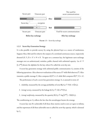
The first information theoretic model that introduces physical layer security was provided by
Wyner in 1975 [107]. The analysis of this model called the degraded wiretap channel introduces
many mathematical tools to consider security constraints in a communication system. As il-
lustrated in Figure 1.1, this model is an extension of the point-to-point channel introduced
by Shannon in which a sender called Alice tries to communicate with a receiver called Bob.
Wyner’s model further considers a third user called Eve that eavesdrops a degraded version of
4

Alice Bob
Eve
Zn
DECENC
Degraded Wiretap
Channel
ˆM
Xn
Y n
pY |X
pZ |Y
M
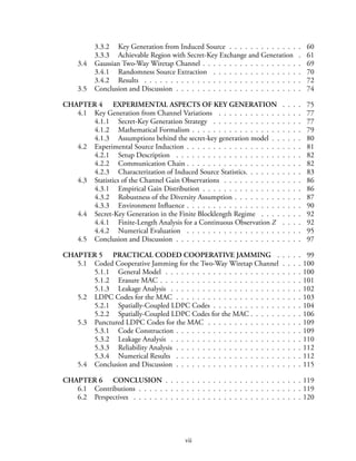
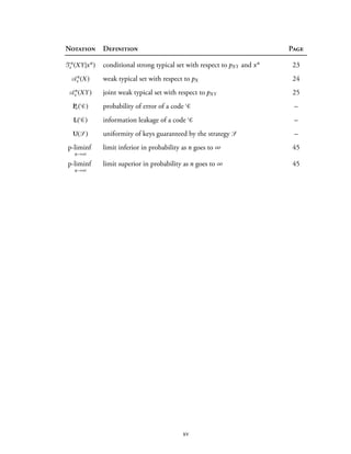
Figure 1.1 – Communications over the degraded wiretap channel.
the main channel output. The objective is to ensure both reliable communications between
Alice and Bob and secrecy with respect to Eve, which should be prevented from getting infor-
mation about transmitted messages.
Mathematically, the channel is a one-input two-output channel with transition probability
pYnZn|Xn , which is, in the case of a memoryless degraded wiretap channel,
pYnZn|Xn (yn
,zn
|xn
) =
n∏
i=1
pY|X
(
y(i)
|x(i)
)
pZ|Y
(
z(i)
|y(i)
)
.
The reliability metric for a wiretap code C is, as usual, the average probability of error
Pe( C) ≜ P( ˆM M| C) between the sent message M and the estimated received message ˆM.
The secrecy metric measures statistical independence with the mutual information I(M;Zn).
For a given code C, the quantity L( C) ≜ I(M;Zn| C) is called the information leakage and
corresponds to a strong secrecy metric. For cases difficult to analyze with a strong secrecy criterion,
there exists a weak secrecy metric called the leakage rate L( C) ≜ 1
n I(M;Zn| C). Leakage rate is a
weaker metric because of the normalization by the blocklength n. Many other metrics can be
considered with different levels of guaranteed security [17].
If sent messages are chosen uniformly at random in a set of 2nR elements, R corresponds to
the rate of the code. A rate is strongly (resp. weakly) achievable if there exists a code C such
that both Pe( C) and L( C) (resp. L( C)) go to zero as n goes to infinity; the supremum of all
achievable rates is called the strong (resp. weak) secrecy capacity of the channel.
In the case of weakly symmetric channels, [60] shows that the secrecy capacity is the differ-
ence between the capacity of the main channel and the capacity of the eavesdropper channel.
5

In particular it means that the secrecy capacity is zero as soon as the eavesdropper’s channel is
less noisy than the main channel—that is, I(X;Y) ⩽ I(X;Z).
2nR0
codewords per subcode
M
M0
codeword
······
······
···
······
···
· · ·
· · ·
· · ·
· · · · · ·
· · ·
· · ·
· · ·
2nRsubcodes
Figure 1.2 – Nested structure of a wiretap code.
Random encoding The crucial part to provide secrecy is to introduce randomness in the
encoder. Intuitively, the randomness is introduced to mislead and confuse the eavesdropper,
but it can be formally proven with information theoretic tools. The randomness is introduced
with a random auxiliary message M′ drawn uniformly at random in 1, 2nR . As represented in
Figure 1.2, a wiretap code has a nested structure: message M selects one of 2nR subcodes and M′
picks a codeword within the 2nR′
possible codewords of the subcode.
Channel capacity Channel resolvability
Xn
Xn
Zn
Zn
Figure 1.3 – Capacity versus resolvability.
Capacity vs. resolvability To find the capacity of a wiretap channel, one has to identify
the optimal auxiliary message R′ rate that introduces enough randomness to mislead the eaves-
dropper without wasting the communication rate. There are two conceptual approaches to
6

deal with this problem, which are illustrated in Figure 1.3. The first called coding for channel
capacity relies on the fact that I(M;Zn) = I(Xn;Zn) − H(M′) + H(M′|MXn). It may seem
logical that H(M′) cancels I(Xn;Zn), if the encoder is random enough; however, dealing with
H(M′|MXn) is far less intuitive. Indeed, to cancel H(M′|MXn) the code must allow a virtual
user obtaining Zn and M to retrieve M′. This can be done if subcodes are capacity-achieving
codes for Eve’s channel with auxiliary rates R′ lower than the eavesdropper’s channel capacity.
The second approach, called coding for channel resolvability, attempts to design subcodes such
that Eve’s output distribution is independent of the sent messages, making them indiscernible.
This time, the solution is to work at auxiliary message rates R′ higher than the eavesdropper’s
channel. Even if both approaches give the same secrecy capacity under a weak secrecy criterion,
it is only possible to provide strong secrecy with resolvability-based codes [17, 64].
1.3 Multi-User Information-Theoretic Security
Alice Bob
EveLegitimate User 1 Legitimate User 2
A
Wireless Bidirectional Communication
Eavesdropper
B
A B
Eavesdropping
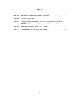
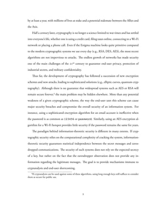
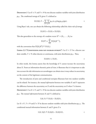
Figure 1.4 – Simple multi-user scheme with eavesdropper.
7

The degraded wiretap channel introduced by Wyner does not take into account several
aspects of muti-user communications. For the sake of illustration, consider the setting repre-
sented in Figure 1.4, which consists of two legitimate users trying to communicate reliably and
secretly with respect to a third-party user that eavesdrops on the conversation. Even if the goals
(reliability and secrecy) are the same as for the wiretap channel, considering bidirectional com-
munications brings new ways of providing secrecy. For instance, the legitimate parties may use
the interference between transmitted signals to “hide” secret information, and the feedback to
exchange side information to “increase” secrecy. A more formal analysis is required to clarify
the notions of “hiding information” and “increasing secrecy”.
Considering a multi-user scheme with two users communicating in two directions as rep-
resented in Figure 1.4 takes into account both feedback and interference. A scheme involving
more users would allow to consider other securing techniques such as relaying [58] or multi-
user secret-key generation [25]. Another limitation related to this model is the assumption that
the eavesdropper doesn’t communicate over the channel. For instance, an active eavesdropper
would be able to jam the communication and interfere with the legitimate users.
1.3.1 Cooperative Jamming and Coded cooperative jamming
A natural attempt to increase secure communication rates consists in jamming Eve with noise
to decrease her signal-to-noise ratio. This strategy, called cooperative jamming (with noise) [62],
forces one user to stop transmitting information to jam the eavesdropper. To overcome this
limitation, Alice and Bob can use codewords whose interference also has a detrimental effect
on Eve without sacrificing as much information rate. This scheme is called coded cooperative
jamming and was introduced by Tekin and Yener [92, 93].
1.3.2 Key Exchange
Key exchange works as follows: one user sacrifices part of its secret rate to transmit a secret-key
to the other, which then uses the secret-key to encrypt a message, thus augmenting its secret
rate. This mechanism illustrated in Figure 1.5 only transfers secure rate from one user to the
other, but does not generate new secrecy.
8

Alice
Bob
Secure part Unsecure part
Secure part Unsecure part
Before key exchange After key exchange
Secret-key encryption
Used for secret communications
Not used for
secret communications
⊕
Figure 1.5 – Secret-key exchange.
1.3.3 Secret-Key Generation Strategy
It is also possible to provide secrecy by using the physical layer as a source of randomness.
Suppose Alice, Bob and Eve observe the outputs of a correlated continuous source, respectively
denoted (X,Y,Z) ∈ X × Y × Z. To agree on a common key, the legitimate users exchange
messages over an authenticated, noiseless, public channel with unlimited capacity. Let K ≜
1, 2nR denote the alphabet for the key, where R is called the secret-key rate.
A secret-key generation strategy with unlimited public communication Sn consists of the
following operations: Alice observesn realizations of the sourceXn while Bob observesZn; Alice
transmits a public message F; Alice computes K(Xn) ∈ K while Bob computes ˆK(Yn, F) ∈ K.
The performance of such a secret-key generation strategy Sn is assessed in terms of:
1. reliability, measured by the average probability of error Pd(Sn) ≜ P(K ˆK|Sn);
2. (strong) secrecy, measured by the leakage L(Sn) ≜ I(K;ZnF|Sn);
3. (strong) uniformity, measured by the quantity U(Sn) ≜ log 2nR − H(K|Sn).
The conditioning on Sn reflects the fact that the eavesdropper knows the strategy.
A secret-key rate R is achievable if all those three metrics tend to zero as n goes to infinity,
and the supremum of all these achievable rates is called the secret-key capacity, which is denoted
by Cs.
9

1.4 Experimental Aspects
The information theory results rely on the existence of random phenomena. For several physical
reasons (noise, environment modifications, mobility, etc.), a wireless channel exhibits some
variability that can be exploited as a source of randomness in a security system. In particular,
one can exploit the reciprocity of wireless channels to generate strongly correlated observations
between two users, and the diversity between channels so that an external eavesdropper obtains
little information about the correlated observations.
Several works, such as [49, 63, 72, 98, 109–111] and references therein, study the problem
of secret-key generation with reconciliation and privacy amplification [9, 67]. They used differ-
ent solutions to induce the source of randomness from the channel (gain, phase, etc.). However,
the security analysis is often performed with metrics (probability of error for the eavesdropper,
NIST tests, decorrelation, etc.) that do not guarantee information-theoretic security. From an
information-theoretic perspective, their analyses do not suffice to ensure secrecy, which is one
of the objectives addressed in the next chapters.
1.5 Contributions
This dissertation extends multiple aspects of multi-user communications from the theoretical
model to practical implementations.
Section 2.3, parts of which have been published in [74], investigates the separation of chan-
nel intrinsic randomness and channel resolvability. The proposed joint exponents are compared
to the tandem exponents obtained with a separate approach. This proves at once, achievability
results for channel intrinsic randomness, random number generation, and channel resolvability.
Chapter 3, parts of which have been published in [76], considers the problem of secure
communications over the two-way wiretap channel under a strong secrecy criterion through a
resolvability-based approach. This also improves on previous works by developing an achievable
region based on strategies that exploit both the interference at the eavesdropper’s terminal and
cooperation between legitimate users. This chapter shows how the artificial noise created by
10

cooperative jamming induces a source of common randomness that can be used for secret-
key agreement. The proposed coding technique shows significant improvements for different
configurations of the Gaussian two-way wiretap channel.
Chapter 4, parts of which have been published in [75], analyzes the practical limitations of
a secret-key generation system from channel gain variations in a narrowband wireless environ-
ment. In particular, different assumptions usually made for theoretical purposes are verified
with an actual system based on software-defined radios. It is important not only to characterize
the source of common randomness induced by channel gain variations, but also to estimate
achievable secret-key rates in the finite key-length regime. The secret-key generation system
based on channel gain variations is extremely sensitive to external modifications of the envi-
ronment, and such system should adapt accordingly to guarantee a given level of information-
theoretic secrecy.
Chapter 5, parts of which have been published in [77], presents a practical coded cooper-
ative jamming scheme for the problem of secure communications over the two-way wiretap
channel. This scheme uses low-density parity-check (LDPC) based codes whose codewords in-
terfere at the eavesdropper’s terminal, thus providing secrecy. This chapter offers a comparison
between constructions based on classical LDPC codes and spatially coupled LDPC codes, and
shows that the latter guarantees low information leakage rate.
11

List of Publications
[74] Pierrot, A. J., Bloch, M. R., “Joint Channel Intrinsic Randomness and Channel Re-
solvability”. In: Proceedings of the 2013 IEEE Information Theory Workshop (ITW). Sept.
2013, pp. 1–5
[76] Pierrot, A. J., Bloch, M. R., “Strongly Secure Communications Over the Two-Way Wire-
tap Channel”. In: IEEE Transactions on Information Forensics and Security 6.3 (Sept.
2011), pp. 595–605
[77] Pierrot, A. J., Bloch, M. R., “LDPC-Based Coded Cooperative Jamming Codes”. In:
Proceedings of the IEEE Information Theory Workshop. Lausanne, Switzerland, Sept. 2012,
pp. 462–466
[75] Pierrot, A. J., Chou, R. A., Bloch, M. R., “Experimental Aspects of Secret Key Genera-
tion in Indoor Wireless Environments”. In: Proceedings of the 14th Workshop on Signal
Processing Advances in Wireless Communications (SPAWC). June 2013, pp. 669–673
12

CHAPTER 2
INFORMATION-THEORETIC SECURITY¹
In this chapter, several metrics are introduced to clarify notation and recall several well-known
properties, which appear with further details in [16, 23]. These information-theoretic proper-
ties are the base to introduce several notions including:
• the channel capacity, which represents the maximum number of bits one can reliably
transmit;
• the problem of source coding with side information, which considers the problem of com-
pression for a correlated source of randomness;
• the channel intrinsic randomness, which defines the maximum uniform randomness that
can be extracted from a channel independently of its input;
• the channel resolvability, which corresponds to the process of transforming a uniform
random number into another one with a different distribution.
All these notions are the essential ingredients to analyze the security of multi-user schemes
and are useful to provide asymptotical limits, error exponents, finite-length results, and insight
into the design of practical systems. In particular, channel intrinsic randomness and source
coding with side information are both essential results for secret-key generation, while channel
resolvability is used to show the fundamental limits of strongly secure schemes.
2.1 Tools of Information Theory
2.1.1 Entropy and Mutual Information
The entropy, which was introduced by Shannon, is a statistical metric of the information, or,
more precisely, of the uncertainty of the outcome of a random variable.
¹Parts of the material in Section 2.3 have appeared in [74]: Pierrot, A. J., Bloch, M. R., “Joint Channel
Intrinsic Randomness and Channel Resolvability”. In: Proceedings of the 2013 IEEE Information Theory Workshop
(ITW). Sept. 2013, pp. 1–5. ©IEEE 2013.
13

Definition 1 Let X ∈ X be a discrete random variable with distribution pX . The Shannon
entropy (or entropy for short) of X is defined as
H(X) ≜ −
∑
x∈X
pX (x) logpX (x) ,
with the convention that 0 log 0 ≜ 0. Unless otherwise specified, all logarithms are taken to
the base two and the unit for entropy is called a bit. ♢
If X = {0, 1}, then X is a binary random variable and its entropy solely depends on the
parameter p = P(X = 0). The binary entropy function is defined as
Hb(p) ≜ −p logp − (1 − p) log(1 − p). (2.1)
For instance for X ∼ B(p), ifp is equal to 1/2 , the uncertainty on X is maximal and Hb(p) = 1.
Lemma 2.1 For any discrete random variable X ∈ X
0 ⩽ H(X) ⩽ log |X| .
The equality H(X) = 0 holds if and only if X is a constant while the equality H(X) = log |X|
holds if and only if X is uniform on X. ♢
This first simple lemma is of primary importance since the notion of uniformity is one of the
pivotal aspects of information-theoretic security. Uniformity corresponds to the maximum
possible uncertainty of a random variable, which is one of the desirable properties for a secret-
key.
The notion of entropy can be further extended to joint and conditional distributions.
Definition 2 Let X ∈ X and Y ∈ Y be two discrete random variables with joint distribution
pXY . The joint entropy of X and Y is defined as
H(XY) ≜ −
∑
x∈X
∑
y∈Y
pXY (x,y) logpXY (x,y) . ♢
14

pXY . The conditional entropy of X given Y is defined as
H(Y|X) ≜ −
∑
x∈X
∑
y∈Y
pXY (x,y) logpY|X (y|x) . ♢
Using Bayes’ rule, one can obtain the following relationship called the chain rule of entropy
H(XY) = H(X) + H(Y|X) .
This also generalizes to the entropy of a random vector Xn = (X1, . . . ,Xn) as
H(Xn
) =
n∑
i=1
H Xi|Xi−1
,
with the convention that H X1|X0 ≜ H(X1).
Lemma 2.2 (“Conditioning does not increase entropy”) Let X ∈ X be a discrete ran-
dom variable, Y ∈ Y either discrete or continuous, with joint distribution pXY . Then,
H(X|Y) ⩽ H(X) . ♢
In other words, this lemma asserts that the knowledge of Y cannot increase the uncertainty
about X. From an information-theoretic point of view, it illustrates that it is important to take
into account the side information an eavesdropper can obtain since it may reduce its uncertainty
on the content of the legitimate communication.
The introduction of joint and conditional entropies illustrates how two random variables
can be related. For instance, the mutual information between two variables X and Y represents
the difference between the uncertainty on X and the uncertainty on X when Y is known.
pXY . The mutual information between X and Y is defined as
I(X;Y) ≜ H(X) − H(X|Y) .
Let X ∈ X, Y ∈ Y and Z ∈ Z be discrete random variables with joint distribution pXYZ . The
conditional mutual information between X and Y given Z is
I(X;Y|Z) ≜ H(X|Z) − H(X|YZ) . ♢
15

The mutual information between X and Y can be also viewed as the expectation of the
following random variable:
I(X;Y) ≜ iX;Y (X;Y) with iX;Y ≜ log
pXY
pXpY
.
Using the chain rule of entropy, one obtains the chain rule of mutual information
I(Xn
;Y) =
n∑
i=1
I Xi;Y|Xi−1
,
with the convention that I X1;Y|X0 ≜ I(X1;Y).
Lemma 2.3 Let X ∈ X and Y ∈ Y be two discrete random variables with joint distribution
pXY . Then,
0 ⩽ I(X;Y) ⩽ min (H(X) , H(Y)) .
The equality I(X;Y) = 0 holds if and only if X and Y are independent. The equality I(X;Y) =
H(X) (resp. I(X;Y) = H(Y)) holds if and only if X is a function of Y (resp. Y is a function
of X). ♢
Along with the notion of uniformity, the notion of independence is also important for
information-theoretic security. Ensuring that the eavesdropper in a security scheme observes
something completely independent of the legitimate communication guarantees the maximum
desirable level of security. Guaranteeing independence avoids justifying security by means of
computational complexity as it is done in classic cryptography.
Lemma 2.4 Let X ∈ X, Y ∈ Y and Z ∈ Z be three discrete random variables with joint
distribution pXYZ . Then,
0 ⩽ I(X;Y|Z) ⩽ min (H(X|Z) , H(Y|Z)) .
The equality I(X;Y|Z) = 0 holds if and only if X and Y are conditionally independent given Z.
In this case, X → Y → Z is called a Markov chain. The equality I(X;Y|Z) = H(X|Z) (resp.
I(X;Y|Z) = H(Y|Z) ) holds if and only if X is a function of Y and Z (resp. Y is a function of
X and Z ). ♢
16

Lemma 2.5 (Data Processing Inequality) Let X ∈ X, Y ∈ Y and Z ∈ Z be three discrete
random variables such that X → Y → Z forms a Markov chain. Then,
I(X;Y) ⩾ I(X;Z). ♢
This inequality is equivalent to H(X|Y) ⩽ H(X|Z), which means that, on average, processing
Y can only increase the uncertainty about X. This property illustrates, for instance, that it is
important not to suppose than the eavesdropper processes its observation to fully assess the
security of a secrecy scheme.
Lemma 2.6 (Fano’s Inequality) Let X ∈ X be a discrete random variable and let ˆX be any
estimate of X that takes values in the same alphabet X. Let Pe ≜ P X ˆX be the probability
of error obtained when estimating X with ˆX. Then,
H X| ˆX ⩽ Hb(Pe) + Pe log(|X| − 1),
where Hb(Pe) is the binary entropy function defined earlier. ♢
Fano’s inequality is another element of several proofs since it relates the information-theoretic
quantity H X| ˆX to an operational quantity, the probability of error Pe.
Since encoding and decoding operations correspond to applying a function to random
variables, it is important to characterize the effects of such processing on the information metrics
mentioned above. If there is no general rule for all the functions, some classes of functions
exhibit interesting behaviors from an information-theoretic perspective. It is, for instance, the
case for convex functions.
Definition 5 A function f : I → R defined on a set I is convex on I if for all (x1,x2) ∈ I2
and for all λ ∈ [0, 1],
f (λx1 + (1 − λ)x2) ⩽ λf (x1) + (1 − λ)f (x2).
If the equation above holds with strict inequality, f is strictly convex on I. A function f :
I → R defined on a set I is (strictly) concave on I if the function −f is (strictly) convex
on I. ♢
17

Applying a convex function to a random variable yields the following properties.
Lemma 2.7 (Jensen’s inequality) Let X ∈ X be a random variable and let f : X → R be a
convex function. Then,
E(f (X)) ⩾ f (E(X)) .
If f is strictly convex, then equality holds if and only if X is a constant. ♢
By exploiting the convexity of − log and Jensen’s inequality, several properties ensue.
pXY . Then
• H(X) is a concave function of pX ;
• I(X;Y) is a concave function of pX for pY|X fixed;
• I(X;Y) is a convex function of pY|X for pX fixed. ♢
2.1.2 Rényi Entropy
There exist several variations of the notion of entropy in the literature. These variations are
useful tools in information theory even if their operational meaning is not as intuitive as the
Shannon entropy or the mutual information. The first variation is called the Rényi entropy [84]
and is meant to be a generalization of the entropy that would preserve fundamental properties,
such as the additivity of independent events.
Definition 6 Let X ∈ X be a discrete random variable with distribution pX . Let ϵ ⩾ 0. The
Rényi entropy of order α ∈ R+{1} of X is defined as
Hα (X) ≜
1
1 − α
log
∑
x∈X
pX (x)α
. (2.2)
♢
One can see the Rényi entropy as a counterpart of the p-norms in Euclidean spaces. The
limit of Hα (X), when α goes to one, is equal to the Shannon entropy H(X). The second
order Rényi entropy is also called the collision entropy (also denoted Hc(X)) and appears in
18

the problem of privacy amplification. The limit of Hα (X) as α goes to infinity is called the
min-entropy
H∞(X) ≜ lim
α→∞
1
1 − α
log
∑
x∈X
pX (x)α
= − log max
x∈X
PX (x). (2.3)
In 2004, Renner and Wolf [83] further extended the notion of Rényi entropy for opera-
tional purposes in secret-key generation.
Definition 7 Let X ∈ X be a discrete random variable with distribution pX . Let ϵ ⩾ 0. The
ϵ-smooth Rényi entropy of order α, with α ∈ R∗
+{1}, of X is defined as
Hϵ
α (X) ≜
1
1 − α
inf
qX ∈Bϵ (X)
log
∑
x∈X
qX (x)α
, (2.4)
where Bϵ(X) ≜ {qX , V(pX ,qX ) ⩽ ϵ} is the set of distributions qX that are ϵ close to pX in
terms of variational distance. ♢
The quantity Hϵ
α (X) converges as α goes to infinity to the ϵ-smooth min-entropy. All these
metrics have conditional formulations [6, 33, 51], in particular for two random variables X
and Y, one definition of the conditional ϵ-smooth min-entropy of X given Y is
Hϵ
∞(X|Y) = max
qXY ∈Bϵ (XY)
min
y∈Y
min
x∈X
log
pY (y)
qXY (XY)
. (2.5)
2.1.3 Other Metrics
The previous section has illustrated the spirit of information theory, which is how one can relate
the notion of information to quantities as abstract as probability distributions. In this section,
several other metrics are introduced, and even if their meaning is not as intuitive as the entropy
or the mutual information, they are primal intermediaries to conduct proofs.
Definition 8 Let X and X′ be two discrete random variables defined on the same alphabet
X. The (total) variational distance between X and X′ is
V(pX ,pX ′) ≜ max
A⊆X
(PX (A) − PX ′(A)) ≡
1
2
∑
x∈X
|pX (x) − pX ′(x)| . ♢
This distance is simply half of the L1 distance between two distributions and all the associ-
ated properties (in particular the triangular inequality) hold.
19

Proposition 2.9 (Triangular inequality) Let X, X′, and X′′ be three discrete random
variables defined on the same alphabet X. Then,
V(pX ,X ′′ ) ⩽ V(pX ,pX ′) + V(pX ′,pX ′′). ♢
There is also a counterpart of the data processing inequality for the variational distance.
Proposition 2.10 (Data Processing Inequality) Let X and X′ be two random variables
defined on the same alphabet X. Consider a function f : X → Y mapping X to Y and X′ to
Y′. Then,
V(pY ,pY ′) ⩽ V(pX ,pX ′). ♢
Fortunately, the variational distance can be related to the entropy through the following
inequality [26].
Proposition 2.11 (Csiszár & Körner) Let X and X′ be two discrete random variables de-
fined on the same alphabet X. Then,
H(X) − H(X′
) ⩽ V(pX ,pX ′) log
|X|
V(pX ,pX ′)
. ♢
This proposition can also relate the mutual information to the variational distance [50].
Corollary 2.12 Let X and Y be two discrete random variables defined on their respective
alphabets X and Y. If card|X| ⩾ 4, then
I(X,Y) ⩽ V(pXY ,pXpY ) log
|X|
V(pXY ,pXpY )
. ♢
Another important metric that relates two probability distributions, without being an actual
distance, is the Kullback-Leiber (KL) divergence.
X. The Kullback-Leiber (KL) divergence between X and X′ is
D(pX ∥pX ′) ≜
∑
x∈X
pX (x) log
pX (x)
pX ′(x)
,
if ∀x ∈ X, pX ′(x) = 0 ⇒ pX (x) = 0, with the convention 0 log 0 = 0. ♢
20

The mutual information can be expressed with the Kullback-Leiber divergence between
specific distributions.
pXY and respective marginal distributions pX and pY . Then
I(X;Y) ≡ D(pXY ∥pXpY ). ♢
The KL divergence also relates to the variational distance through Pinsker’s inequality [26, 78].
Proposition 2.14 (Pinsker) Let X and X′ be two discrete random variables defined on the
same alphabet X. Then,
V(pX ,pX ′) ⩽
√
2ln(2)D(pX ∥pX ′). ♢
Similar to the entropy, the KL divergence can also be extended to a Rényi divergence [84].
X. The Rényi divergence of order α ∈ R∗
+{1}, between X and X′ is
Dα (pX ||pX ′) ≜
1
α − 1
log
∑
x∈X
pX (x)α
qX (x)1−α
,
with the conventions 0/0 = 0 and x/0 = ∞ for x 0. ♢
Note that, when α goes to one, the Rényi divergence is strictly equivalent to the Kullback-
Lever divergence. The reader is invited to refer to [30] for a complete list of properties for the
Rényi divergence.
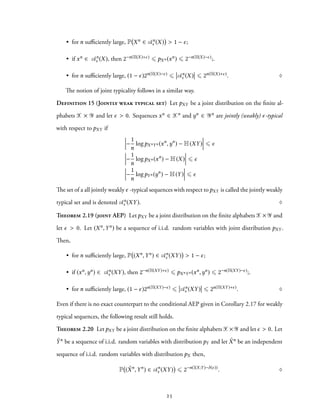
2.1.4 Typical Sequences
The notion of typical sequence is at the center of information theory proofs. Intuitively, a
typical sequence is a sequence whose statistics are representative of the behavior of its associated
random variable. These sequences have interesting properties presented in this subsection. Two
notions of typicality exist: the strong typicality is the most intuitive, while the weak typicality
is mostly an information theory concept.
2.1.4.1 Strongly Typical Sequences
Let xn ∈ Xn be a sequence whose n elements are in a finite alphabet X.
21

Notation N(a;xn) denotes the number of occurrences of a symbol a ∈ X in the sequence
xn, and {N(a;xn)/n : a ∈ X} represents the empirical distribution of xn.
Definition 11 (Strong typical set) Let pX be a distribution on a finite alphabet X and let
ϵ > 0. A sequence xn ∈ Xn is (strongly) ϵ-typical with respect to pX if
∀a ∈ X
1
n
N(a;xn
) − pX (a) ⩽ ϵ pX (a) .
The set of all ϵ-typical sequences with respect topX is called the strong typical set and is denoted
by Tn
ϵ (X). ♢
This definition is quite intuitive since a typical sequence has an empirical distribution “close”
topX . Typical sequences are particularly useful in information theory because of a result known
as the asymptotic equipartition property (AEP for short).
Theorem 2.15 (AEP) Let pX be a distribution on a finite alphabet X and let 0 < ϵ <
minx∈X pX (x). Let Xn be a sequence of independent and identically distributed (i.i.d.) random
variables with distribution pX . Then,
1 − δϵ(n) ⩽ P Xn
∈ Tn
ϵ (X) ⩽ 1
(1 − δϵ(n))2n(H(X)−δ(ϵ))
⩽ Tn
ϵ (X) ⩽ 2n(H(X)+δ(ϵ))
∀xn
∈ Tn
ϵ (X) 2−n(H(X)+δ(ϵ)
⩽ pXn (xn
) ⩽ 2−n(H(X)−δ(ϵ))
. ♢
The three inequalities given in this theorem can be translated as:
1. for n sufficiently large, the probability that a sequence is strongly typical is close to one;
2. the number of strongly typical sequences is close to 2−nH(X), making a direct connection
with the entropy of a random variable;
3. strongly typical sequences are almost uniformly distributed.
Remark There exist explicit expressions forδϵ(n) andδ(ϵ) [55], but the rough characterization
used in Theorem 2.15 is sufficient for the subsequent analysis. The exact dependence on n
22

or ϵ is not needed because of some operational properties such as δ(ϵ) ± δ(ϵ) = δ(ϵ) and
δϵ(n) ± δϵ(n) = δϵ(n).
The notion of typicality generalizes to multiple random variables. Assume that (xn,yn) ∈
Xn × Yn is a pair of sequences with elements in finite alphabets X and Y. The number of oc-
currences of a pair (a,b) ∈ X× Y in the pair of sequences (xn,yn) is denoted by N(a,b;xn,yn).
Definition 12 (Jointly typical set) Let pXY be a joint distribution on the finite alphabet
X × Y and let ϵ > 0. Sequences xn ∈ Xn and yn ∈ Yn are ϵ-jointly typical with respect to
pXY if
∀(a,b) ∈ X × Y
1
n
N(a,b;xn
,yn
) − pXY (a,b) ⩽ ϵ pXY (a,b) .
The set of all ϵ-jointly typical sequences with respect to pXY is called the jointly typical set and
is denoted by Tn
ϵ (XY). ♢
Since Tn
ϵ (XY) ⊆ Tn
ϵ (X) × Tn
ϵ (Y), if two sequences xn and yn are jointly typical, then they are
also individually typical. The following corollary of Theorem 2.15 is a direct consequence of
this property.
Corollary 2.16 (Joint AEP) Let pXY be a joint distribution on the finite alphabets X × Y
and let 0 < ϵ < min(x,y)∈X×Y pXY (x,y). Let (Xn,Yn) be a sequence of i.i.d. random variables
with joint distribution pXY . Then,
1 − δϵ(n) ⩽ P (Xn
,Yn
) ∈ Tn
ϵ (XY) ⩽ 1
(1 − δϵ(n))2n(H(XY)−δ(ϵ))
⩽ Tn
ϵ (XY) ⩽ 2n(H(XY)+δ(ϵ))
∀(xn
,yn
) ∈ Tn
ϵ (XY) 2−n(H(XY)+δ(ϵ))
⩽ pXnYn (xn
,yn
) ⩽ 2−n(H(XY)−δ(ϵ))
. ♢
A conditional version of the AEP exists for conditional typical sets.
Definition 13 Let pXY be a joint distribution on the finite alphabets X × Y and let ϵ > 0.
Let xn ∈ Tn
ϵ (X). The set
Tn
ϵ (XY|xn
) ≜ yn
∈ Yn
: (xn
,yn
) ∈ Tn
ϵ (XY)
23

called the conditional typical set with respect to xn. ♢
Theorem 2.17 (Conditional AEP) Let pXY be a joint distribution on the finite alphabets
X × Y and suppose 0 < ϵ′ < ϵ ⩽ min(x,y)∈X×Y pXY (x,y). Let xn ∈ Tn
ϵ′(X) and let ˜Yn be a
sequence of random variables such that
∀yn
∈ Yn
p ˜Yn (yn
) =
n∏
i=1
pY|X (yi|xi) .
Then,
1 − δϵϵ′(n) ⩽ P ˜Yn
∈ Tn
ϵ (XY|xn
) ⩽ 1
(1 − δϵϵ′(n))2n(H(Y|X)−δ(ϵ))
⩽ Tn
ϵ (XY|xn
) ⩽ 2n(H(Y|X)+δ(ϵ))
∀yn
∈ Tn
ϵ (XY|xn
) 2−n(H(Y|X)+δ(ϵ))
⩽ pYn|Xn (yn
|xn
) ⩽ 2−n(H(Y|X)−δ(ϵ))
. ♢
2.1.4.2 Weakly Typical Sequences
Even if the notion of strong typicality is intuitive, it does not apply to continuous random vari-
ables. A weaker definition exists to cope with continuous random variables [23] by defining a
typical sequence as a sequence whose empirical entropy is close to the true entropy of the corre-
sponding random variable. The discrete formulation also has practical operational advantages,
which will be exploited in the subsequent chapters.
Definition 14 (Weakly typical set) Let pX be a distribution on a finite alphabet X and let
ϵ > 0. A sequence xn ∈ Xn is (weakly) ϵ-typical with respect to pX if
−
1
n
logpXn (xn
) − H(X) ⩽ ϵ.
The set of a all weakly ϵ-typical sequences with respect to pX is called the weakly typical set and
is denoted An
ϵ (X). ♢
For weak typicality, the AEP is directly obtained from the weak law of large numbers.
Theorem 2.18 (AEP) Let pX be a distribution on a finite alphabet X and let ϵ > 0. Let
Xn be a sequence of independent and identically distributed (i.i.d.) random variables with
distribution pX . Then,
24

• for n sufficiently large, P Xn ∈ An
ϵ (X) > 1 − ϵ;
• if xn ∈ An
ϵ (X), then 2−n(H(X)+ϵ) ⩽ pXn (xn) ⩽ 2−n(H(X)−ϵ);.
• for n sufficiently large, (1 − ϵ)2n(H(X)−ϵ) ⩽ An
ϵ (X) ⩽ 2n(H(X)+ϵ). ♢
The notion of joint typicality follows in a similar way.
Definition 15 (Jointly weak typical set) Let pXY be a joint distribution on the finite al-
phabets X × Y and let ϵ > 0. Sequences xn ∈ Xn and yn ∈ Yn are jointly (weakly) ϵ-typical
with respect to pXY if
−
1
n
logpXnYn (xn
,yn
) − H(XY) ⩽ ϵ
−
1
n
logpXn (xn
) − H(X) ⩽ ϵ
−
1
n
logpYn (yn
) − H(Y) ⩽ ϵ
The set of a all jointly weakly ϵ -typical sequences with respect topXY is called the jointly weakly
typical set and is denoted An
ϵ (XY). ♢
Theorem 2.19 (joint AEP) Let pXY be a joint distribution on the finite alphabets X× Y and
let ϵ > 0. Let (Xn,Yn) be a sequence of i.i.d. random variables with joint distribution pXY .
Then,
• for n sufficiently large, P (Xn,Yn) ∈ An
ϵ (XY) > 1 − ϵ;
• if (xn,yn) ∈ An
ϵ (XY), then 2−n(H(XY)+ϵ) ⩽ pXnYn (xn,yn) ⩽ 2−n(H(XY)−ϵ);.
• for n sufficiently large, (1 − ϵ)2n(H(XY)−ϵ) ⩽ An
ϵ (XY) ⩽ 2n(H(XY)+ϵ). ♢
Even if there is no exact counterpart to the conditional AEP given in Corollary 2.17 for weakly
typical sequences, the following result still holds.
Theorem 2.20 LetpXY be a joint distribution on the finite alphabetsX× Y and let ϵ > 0. Let
˜Yn be a sequence of i.i.d. random variables with distribution pY and let ˜Xn be an independent
sequence of i.i.d. random variables with distribution pX then,
P ( ˜Xn
,Yn
) ∈ An
ϵ (XY) ⩽ 2−n(I(X;Y)−δ(ϵ))
. ♢
25

2.1.5 Markov Chains and Functional Dependence Graphs
For some information theoretic models and coding schemes, it may be rather difficult to de-
scribe the different relationships between random variables. A functional dependence graph is
a convenient tool to analyze these possibly complicated relationships by graphically identifying
the different Markov chains.
XnXi
M
YnYiY1
ZnZiZ1
X1
Figure 2.1 – Functional dependence graph of Example 2.1.5. Independent random variables are indicated
by •, while functions of these random variables are indicated by ◦.
Definition 16 (Functional dependence graph) Form independent random variables and
n functions of these variables, a functional dependence graph is a directed graph withm+n ver-
tices. Each edge between two nodes represents the existence of a mapping between two random
variables. ♢
Example Let M ∈ M and Zn ∈ Rn be two independent random variables, and {fi}n be a
set of functions from M to Rn. For i ∈ 1,n , define the random variables Xi = fi(M) and
Yi = Xi + Zi. The functional dependence graph of the random variables M, Xn
i , Yn
i , and Zn
i is
illustrated in Figure 2.1.
Definition 17 (d-separation) LetX, Y, and Z be disjoint subsets of vertices in a functional
dependence graph G. The subsetZ is said to d-separateX from Y if there exists no path between
a vertex of X and a vertex of Y after the following operations have been performed:
26

• construct the subgraph G′ consisting of all vertices in X, Y, and Z, as well as the edges
and vertices encountered when moving backward starting from any of the vertices in X,
Y, or Z;
• in the subgraph G′, delete all edges coming out of Z;
• remove all arrows in G′ to obtain an undirected graph. ♢
The usefulness of d-separation is justified by the following theorem.
Theorem 2.21 Let X, Y, and Z be disjoint subsets of the vertices in a functional dependence
graph. If Z d-separates X from Y, and if one collects the random variables in X, Y, and Z,
in the random vectors X, Y, and Z, respectively, then X → Z → Y forms a Markov chain. ♢
Theorem 2.21 is particularly useful in the converse proofs of channel coding theorems.
Example From the functional dependence graph of Figure 2.1, for any i j Xi → Xj → Yj.
2.1.6 Information-Theoretic Bounds
Some additional inequalities are useful to bound the probabilities of rare events.
Lemma 2.22 (Markov’s inequality) Let X be a non-negative real-valued random variable.
Then,
∀a > 0 P(X ⩾ a) ⩽
EX (X)
a
. ♢
This Lemma induces a result that is useful in the code selection step of achievability proofs
relying on a random code generation.
Lemma 2.23 (Selection lemma) Let Xn ∈ Xn be a random variable and let F be a finite set
of functions f : Xn → R+ such that |F| does not depend on n and
∀f ∈ F EXn (f (Xn)) ⩽ δ(n).
Then, there exists a specific realization xn of Xn such that
∀f ∈ F f (xn) ⩽ δ(n). ♢
Another useful consequences of Markov’s is the Chernoff bound.
27

Lemma 2.24 (Chernoff bound) Let X be a real-valued random variable. For all a > 0,
∀s > 0 P(X ⩾ a) ⩽ EX esX
e−sa
,
∀s < 0 P(X ⩽ a) ⩽ EX esX
e−sa
. ♢
2.2 Coding Primitives
The previous section provides the necessary tools to analyze many communication systems
from an information-theoretic perspective. This section introduces four fundamental primi-
tives: channel capacity, source coding with side information, channel intrinsic randomness,
and channel resolvability. The analysis of multi-user communications relies on several of these
primitives, which introduces the pivotal proof mechanisms used throughout this dissertation.
The example of point-to-point communications illustrates the fundamental aspects of these
coding primitives.
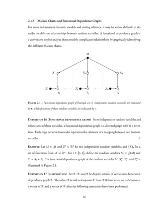
2.2.1 Channel Capacity
Introducing security constraints in the communication model does not mean ignoring the prob-
lem of reliability in communications. The goal is indeed twofold: providing reliable communi-
cations for the legitimate users, and ensuring security with respect to an external eavesdropper.
The problem of reliable point-to-point communications has been introduced by Shannon in
his seminal work [88] and was studied extensively for other channels (esp. the multiple-access
channel).
Xn
ENC DECM
Yn
ˆMpY |X
Figure 2.2 – Point-to-point communications.
The channel capacity for the problem of point-to-point communications depicted in Fig-
ure 2.2 is defined as the maximum bit rate a user can reliably transmit on a noisy channel.
28

Theorem 2.25 (Channel Coding Theorem) The capacity of a discrete memoryless channel
(DMC) X,pY|X , Y is
C = max
pX
I(X;Y).
In other words, if R < C then R is an achievable transmission rate and an achievable transmis-
sion rate must satisfy R ⩽ C. ♢
Theorem 2.25 proves that the channel capacity is equal to the maximum over all possi-
ble input distributions of the mutual information between the channel input and the channel
output.
The proof of this theorem relies on a random coding argument, which consists in drawing
the symbols of codewords independently at random. Showing that there exists a code such that
the probability of error goes to zero as n (the code blocklength) goes to infinity yields an upper
bound on the transmission rate. This random code is only a technical tool and not a practical
code that can be used as an actual coding scheme. The mechanisms presented in the following
achievability proof are essential to tackle more complicated models.
Input Output Input Output
Binary Symmetric
Channel
Binary Erasure
Channel
0
1
0
1
0
1
0
1
?
p
1 p
1 p
p
1
1
Figure 2.3 – Binary symmetric channel and binary erasure channel.
Example Figure 2.3 depicts two binary channels that are particularly useful in information
theory. The binary symmetric channel BSC(p) flips bit values with a crossover probability p
and has a capacity of 1 − Hb(p) bits. The binary erasure channel BEC(ϵ) erases bits a with a
probability ϵ and has a capacity of 1 − ϵ bits.
29

The additive white Gaussian noise (AWGN) channel also has a prominent role in informa-
tion and communication theory to describe a practical communication scheme. The AWGN
channel captures, in particular, the impact of thermal noise and interferences in wireless com-
munications. The channel output at each instant i ⩾ 1 is Yi = Xi + Ni, where Xi denotes the
transmitted symbol and {Ni}i⩾1 are i.i.d. random variables with distribution N(0,σ2). With-
out further restriction the capacity of the AWGN channel is infinite; however, by adding an
average power constraint in the form of
1
n
n∑
i=1
E X2
i ⩽ P,
, the capacity becomes finite.
Theorem 2.26 The capacity of a Gaussian channel is given by
C =
1
2
log
(
1 +
P
σ2
)
,
where P denotes the power constraint and σ2 is the variance of the noise. ♢
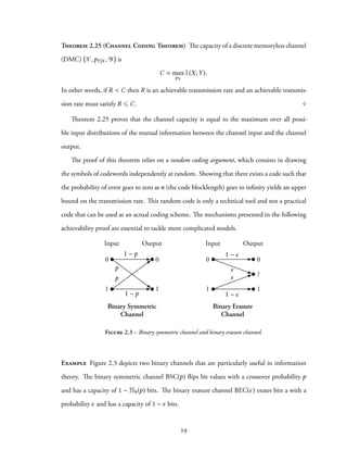
2.2.2 Source Coding with Side Information
Along with channel coding, the problem of source compression is at the core of information
theory. Information-theoretic tools are used to derive fundamental limits regarding the bit rate
at which a source can be compressed without any loss. For instance, for a source (X,pX ), the
minimum number of bits that must be stored or transmitted is nH(X), where n is the length
of the source sequence.
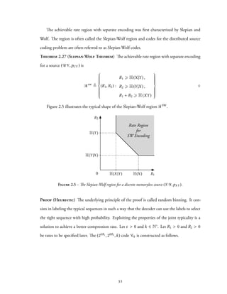
The fundamental paper by Slepian and Wolf [89] considers the separate encoding of corre-
lated sources as illustrated in Figure 2.4.
DEC
ENC
ENC
Xn
Yn
⇣
ˆXn
, ˆYn
⌘
R1
R2
pX,Y
Figure 2.4 – Separate encoding of correlated sources (Slepian-Wolf problem).
30

Consider a DMS (XY,pXY ) with two outputs X and Y with joint distribution pXY . As
depicted in Figure 2.4, the outputs are processed by two different encoders that compress Xn
into a message of rate R1 and compresses Yn into a message of rate R2. Both these messages are
processed jointly by a single decoder, whose goal is to estimate Xn and Yn. Since this model
considers two different encoders one can expect that the best thing to do is to encode X at a
rate R1 > H(X) and Y at a rate R2 > H(Y). This procedure guarantees that the probability
of error vanishes as n goes to infinity but exploits neither the correlation of the source nor the
common decoder. It turns out that it suffices to ensure that the sum rate R1 +R2 is greater than
H(XY), which is in general smaller than H(X)+H(Y). To achieve such a surprising result the
encoders and the decoder must be properly designed [16, 23, 89].
Definition 18 A (2kR1, 2kR2,k) distributed source code Ck for the discrete memoryless source
(XY,pXY ) consists of
• two message sets M1 = 1, 2R1 and M2 = 1, 2nR2 ;
• an encoding function f1 : Xk → M1, xk → m1;
• an encoding function f2 : Yk → M2, yk → m2;
• a decoding function д : M1 × M2 → (Xk × Yk) ∪ {?}, (m1,m2) → (ˆxk, ˆyk), where ?
represents the error symbol. ♢
The performance of a code Ck is measured in terms of the average probability of error
Pe( Ck) ≜ P
(
( ˆXk
, ˆYk
) (Xk
,Yk
) Ck
)
.
Definition 19 A rate pair (R1,R2) is achievable if there exists a sequence of (2kR1, 2kR2,k)
codes { Ck}k⩾1 such that
lim
k→∞
Pe( Ck) = 0.
The achievable rate region is defined as
Rsw
≜ cl({(R1,R2) : (R1,R2) is achievable}) . ♢
31

The achievable rate region with separate encoding was first characterized by Slepian and
Wolf. The region is often called the Slepian-Wolf region and codes for the distributed source
coding problem are often referred to as Slepian-Wolf codes.
Theorem 2.27 (Slepian-Wolf Theorem) The achievable rate region with separate encoding
for a source (UV,pUV ) is
Rsw
≜



(R1,R2) :
R1 ⩾ H(X|Y) ,
R2 ⩾ H(Y|X) ,
R1 + R2 ⩾ H(XY)



♢
Figure 2.5 illustrates the typical shape of the Slepian-Wolf region RSW.
R1
R2
Rate Region
for
SW Encoding
0
H(Y |X )
H(X |Y ) H(X )
H(Y )
Figure 2.5 – The Slepian-Wolf region for a discrete memoryless source (XY,pXY ).
Proof (Heuristic) The underlying principle of the proof is called random binning. It con-
sists in labeling the typical sequences in such a way that the decoder can use the labels to select
the right sequence with high probability. Exploiting the properties of the joint typicality is a
solution to achieve a better compression rate. Let ϵ > 0 and k ∈ N∗. Let R1 > 0 and R2 > 0
be rates to be specified later. The (2kR1, 2kR2,k) code Ck is constructed as follows.
32

• Binning: For each sequence xk ∈ Tk
ϵ (X), draw an index uniformly at random in the set
1, 2kR1 . For each sequence yk ∈ Tk
ϵ (Y), draw an index uniformly at random in the set
1, 2kR2 . The index assignments define the encoding functions
f1 : Xk
→ 1, 2kR1
and f2 : Yk
→ 1, 2kR2
,
which are revealed to all parties.
• Encoder 1: given the observation xk, if xk ∈ Tk
ϵ (X), output m1 = f1(xk); otherwise
output m1 = 1.
• Encoder 2: given the observation yk, if yk ∈ Tk
ϵ (Y), output m2 = f2(yk); otherwise
output m2 = 1.
• Decoder: given messages m1 and m2, output ˆxk and ˆyk if they are the unique sequences
such that (ˆxk, ˆyk) ∈ Tk
ϵ (XY) and f1(ˆxk) = m1, f2(ˆyk) = m2; otherwise, output ?.
. . .
. . .
. . .
...
...
...
...
...
...
...
2nR1 bins for xn
2nR2binsforn
Figure 2.6 – Binning procedure for the Slepian-Wolf coding. Each pictogram represents one of the 2nH(XY )
jointly typical pairs (xn,yn).
Figure 2.6 represents how the binning procedure work. The bins are designed in such a
way that each of the 2nH(XY) jointly typical pairs (xn,yn) receives a unique pair of indices. The
reader is invited to refer to [16, 23] for the detailed technical proof.
33

One of the special cases of the Slepian-Wolf problem consists in supposing that one the
components of the DMS (XY,pXY ), say Y, is directly available at the decoder as side infor-
mation and only X should be compressed. This problem is known as source coding with side
information.
Corollary 2.28 (Source coding with side information) Consider a DMS (XY,pXY )
and assume that (X,pX ) should be compressed knowing that (Y,pY ) is available as side infor-
mation at the decoder. Then,
inf{R : R is an achievable compression rate} = H(X|Y) . ♢
This result confirms that a source with low entropy can be compressed more than a source
with higher entropy. Corollary 2.28 plays a pivotal role in physical layer security and, in par-
ticular, for secret-key generation. To distill a secret-key from the physical medium, two users
must observe a correlated source of randomness. This correlated source of randomness does not
provide identical observations, thus requiring a reconciliation procedure. To agree on a com-
mon key, the two users exchange messages that allow them to agree on a common sequence,
which is then used to distill a key. Source coding with side information generalizes the problem
of source coding when additional side information is available either to both users or only one.
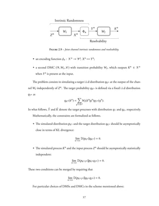
2.2.3 Channel Intrinsic Randomness
Zn Xn
n YnpX |Z
Figure 2.7 – Channel Intrinsic Randomness (CIR) basic scheme.
The Channel Intrinsic Randomness (CIR for short) is defined in [13] as the “maximum
bit rates that can be extracted from a channel output independently of an input with known
statistics.” This problem is of primary importance to analyze secret-key generation schemes to
provide strong security.
34

Formally, consider a discrete memoryless channel (Z,X,pX|Z ), and suppose that the dis-
tribution controlling the channel is pZ . Channel intrinsic randomness consists in designing a
mapping φn such that, for any ϵ > 0
V pZnφn(Xn),pZnqYn ⩽ ϵ,
where qYn represents a desired target distribution. For an arbitrary distribution qYn is called
channel number generation.
The following proposition yields a condition on the process {Yn}n⩾1 to ensure the existence
of such a mapping φn.
Proposition 2.29 (Achievability of CIR) If H(X|Z) > H(Y), then
∀0 < ϵ < 0.1, ∃φn : Xn
→ Yn
, V pZnφn(Xn),pZnqYn ⩽ ϵ, (2.6)
and
∀0 < ϵ < 0.1, ∃φ′
n : Xn
→ Yn
, D pZnφn(Xn)∥pZnqYn ⩽ ϵ. (2.7)
♢
In [13], the author presents a result that holds for sources with memory, but all the analysis
done in the subsequent chapters will only focus on channels without memory.
Proof This results can be proven as a corollary of Corollary 2.31 and Pinsker’s inequality.
2.2.4 Channel Resolvability
Xn
n
Yn
KnpK |Y
Figure 2.8 – Channel Resolvability basic scheme.
The paradigm behind the wiretap coding consists in ensuring that the observation of the
eavesdropper is independent of the secret messages. A sufficient way to guarantee security con-
sists in ensuring that the eavesdropper’s statistics are not affected by the messages exchanged by
the legitimate parties. In that case, the eavesdropper cannot resolve what message was transmit-
ted since it doesn’t observe significant variations on its end. This approach called channel resolv-
ability ensures strongly secure communications, while capacity based approaches only provide
35

weak secrecy. Channel resolvability [39] aims at simulating a target distribution at the output
of a channel by controlling its input with a uniform random number.
Formally, consider a discrete memoryless channel (Y, K,pK|Y ), and suppose that the dis-
tribution controlling the channel is pK. Channel intrinsic randomness consists in designing a
mapping φn such that, for any ϵ > 0
V pZnφn(Xn),pZnpKn ⩽ ϵ. (2.8)
The same result holds for the KL divergence.
2.3 Joint Analysis of Channel Intrinsic Randomness and Resolvability
This section introduces a scheme that includes and extends the problems of channel resolvability
and channel intrinsic randomness. The model consists of a discrete memoryless source that is
sent through a first discrete memoryless channel, which output is then processed to feed the in-
put of a second channel. The objective is to simulate a random process with fixed distribution at
the second channel output independently from the first channel input. A joint scheme is intro-
duced to find joint exponents and asymptotic limits that can be specialized to the well-known
schemes previously mentioned. This scheme also provides, for instance, a direct extension of
channel intrinsic randomness with a non-uniform target distribution.
The joint approach does not improve asymptotic limits since separation holds in some cases,
but the joint exponents are larger than the tandem exponents that would be obtained by using
an intermediate uniform random number. Even if the model is more general, the subsequent
results are connected to some of the separation approaches investigated in [96, 97] and to
channel resolvability with non-uniform input [14, 42].
2.3.1 Deﬁnitions and Assumptions
Consider the setting illustrated in Figure 2.9 consisting of:
• a discrete memoryless source (DMS) (Z,qZ ) that outputs i.i.d. sequences Zn ∈ Zn;
• a discrete memoryless channel (DMC) (Z,W1,X) with transition probabilityW1, which
outputs i.i.d sequences Xn ∈ Xn when Zn is present at the input;
36

Intrinsic Randomness
Resolvability
Zn
W1
Xn
n
Yn
W2
Kn
Figure 2.9 – Joint channel intrinsic randomness and resolvability.
• an encoding function φn : Xn → Yn, Xn → Yn;
• a second DMC (Y,W2, K) with transition probability W2, which outputs Kn ∈ Xn
when Yn is present at the input.
The problem consists in simulating a target i.i.d distribution qKn at the output of the chan-
nel W2 independently of Zn. The target probability qKn is defined via a fixed i.i.d distribution
qYn as
qKn (kn
) =
∑
yn ∈Yn
W2(kn
|yn
)qYn (yn
).
In what follows, ˜Y and ˜K denote the target processes with distribution qY and qK, respectively.
Mathematically, the constraints are formalized as follows.
• The simulated distribution pKn and the target distribution qKn should be asymptotically
close in terms of KL divergence:
lim
n→∞
D(pKn ||qKn ) = 0.
• The simulated process Kn and the input process Zn should be asymptotically statistically
independent:
lim
n→∞
D(pKnZn ||pKnqZn ) = 0.
These two conditions can be merged by requiring that
lim
n→∞
D(pKnZn ||qKnqZn ) = 0.
For particular choices of DMSs and DMCs in the scheme mentioned above:
37

• if Y = K, W2 = idK, and qKn ∼ U 1, 2nR , it corresponds to channel intrinsic random-
ness;
• if W1 = qX , qXn ∼ U 1, 2nR , it corresponds to channel resolvability.
2.3.2 Achievability and Exponents
2.3.2.1 Joint Exponent Derivation
The joint exponent derivation derives from a proof technique introduced by Hayashi [40, 41]
(see also [48]). First, the joint coding scheme is constructed at random; the encoding function
φn is randomly defined by mapping every sequence xn ∈ Xn to a sequence yn ∈ Yn drawn
according to qYn . The corresponding random variable is denoted Φn.
For 0 < α < 1,
D(pKnZn ||qKnqZn )
(a)
⩽
∑
zn ∈Zn
qZn (zn
)D(pKn|Zn=zn ||qKn )
(b)
⩽
∑
zn ∈Zn
qZn (zn
)D1+α (pKn|Zn=zn ||qKn ), (2.9)
Inequality (a) follows from the law of total probability, and (b) holds because the Rényi
divergence is increasing with respect to α (see for instance [29]).
By taking the expectation of inequality (2.9), over all encoding function Φn and with
Jensen’s inequality,
EΦn (D(pKnZn ||qKnqZn ))
⩽
1
α
∑
zn ∈Zn
qZn (zn
) × log
∑
kn ∈Kn
qKn (kn
)−α
EΦn pKn|Zn (kn
|zn
)1+α
. (2.10)
By the law of total probability and observing that Zn → Xn → Yn → Kn forms a Markov
chain and for a given realization φn of Φn,
pKn|Zn (kn
|zn
) =
∑
yn ∈Yn
W2(kn
|yn
)
∑
xn ∈Xn
W1(xn
|zn
)1 {φn(xn
) = yn
} . (2.11)
38

Therefore,
EΦn pKn|Zn (kn
|zn
)1+α
=
∑
xn ∈Xn
∑
yn ∈Yn
∑
φn(xn)∈Yn
qYn (φn(xn
))W1(xn
|zn
)W2(kn
|yn
)1 {φn(xn
) = yn
}
× Exn
Φn
∑
˜xn, ˜yn
W1( ˜xn
|zn
)W2(kn
| ˜yn
)1 {φn( ˜xn
) = ˜yn
}
α
, (2.12)
where Exn
Φn
is the expectation over all possible mapping Φn where the value φn(xn) is fixed. This
expectation can be upper bounded as follows
Exn
Φn
∑
˜xn, ˜yn
W1( ˜xn
|zn
)W2(kn
| ˜yn
)1 {φn( ˜xn
) = ˜yn
}
α
(a)
⩽ Exn
Φn
(W1(xn
|zn
)W2(kn
|yn
)1 {φn(xn
) = yn
})α
+ Exn
Φn
∑
˜xn xn
∑
˜yn yn
W1( ˜xn
|zn
)W2(kn
| ˜yn
)1 {φn( ˜xn
) = ˜yn
}
α
(b)
⩽ (W1(xn
|zn
)W2(kn
|yn
))α
+
∑
˜xn xn
∑
˜yn yn
Exn
Φn
(W1( ˜xn
|zn
)W2(kn
| ˜yn
)1 {φn( ˜xn
) = ˜yn
})
α
(c)
⩽ (W1(xn
|zn
)W2(kn
|yn
))α
+
( ∑
˜xn xn
W1( ˜xn
|zn
)
=1
∑
˜yn yn
W2(kn
| ˜yn
)qYn ( ˜yn
)
qKn (kn)
)α
⩽ (W1(xn
|zn
)W2(kn
|yn
))α
+ qKn (kn
)α
. (2.13)
Inequality (a) is obtained by splitting the sum and because x → xα is concave for 0 < α <
1; inequality (b) because of Jensen’s inequality and 1 {φn(xn) = yn} ⩽ 1; and inequality (c)
because Exn
Φn
(1 {φn( ˜xn) = ˜yn}) = qYn ( ˜yn) for ˜xn xn.
39

Plugging (2.13) into (2.12), yields after some calculations,
EΦn pKn|Zn (kn
|zn
)1+α
⩽ qKn (kn
)1+α
(
1 +
∑
xn ∈Xn
W1(xn
|zn
)1+α
∑
yn ∈Yn
qYn (yn
)
(
W2(kn|yn)
qKn (kn)
)1+α )
. (2.14)
EΦn (D(pKnZn ||qKnqZn ))
⩽
1
α
∑
zn ∈Zn
qZn (zn
)
× log
∑
kn ∈Kn
qKn (kn
) 1 +
∑
xn ∈Xn
W1(xn
|zn
)1+α
∑
yn ∈Yn
qYn (yn
)
(
W2(kn|yn)
qKn (kn)
)1+α
⩽
1
α
log 1 +
∑
zn ∈Zn
∑
kn ∈Kn
qZn (zn
)qKn (kn
)
∑
xn ∈Xn
W1(xn
|zn
)1+α
∑
yn ∈Yn
qYn (yn
)
(
W2(kn|yn)
qKn (kn)
)1+α
⩽
1
α
∑
kn ∈Kn
∑
yn ∈Yn
W2(kn
|yn
)1+α
qYn (yn
)qKn (kn
)−α
∑
zn ∈Zn
∑
xn ∈Xn
W1(xn
|zn
)1+α
qZn (zn
) (2.15)
Exponentinnats
Tandem exponent……
Joint exponent
Parameter
Figure 2.10 – Comparison of joint and tandem exponents for different values ofκ when ω = 0.3, for channel
intrinsic randomness and source resolvability.
Finally, equation (2.15) brings the following proposition
40

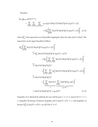
Proposition 2.30 There exists a mapping φn : Xn → Yn, such that
D(pKnZn ||qKnqZn ) ⩽ e−nEj (qZ ,qK ,W1,W2)
,
with
Ej(qZ ,qK,W1,W2) = max
α∈[0,1]
Ec(α,qZ ,W1) − Er (α,qY ,W2), (2.16)
and
Ec(α,qZ ,W1) = − log
∑
z∈Z
qZ (z)
∑
x∈X
W1(x|z)1+α
Er (α,qY ,W2) = log
∑
k∈K
∑
y∈Y
W2(k|y)1+α
qY (y)qK(k)−α
. (2.17)
♢
Remark Using the same upper bound as in [41],
Er (α,qY ,W2) ⩽ log
∑
kn ∈Kn
∑
yn ∈Yn
qYn (yn
)W2(kn
|yn
)
1
1−α
1−α
≜ E′
r (α,qY ,W2). (2.18)
Corollary 2.31 If H(X|Z) ⩾ I( ˜Y; ˜K), then there exists a mapping φn : X → Y, such that
lim
n→∞
D(pKnZn ||qKnqZn ) = 0.
♢
Proof The key behind the asymptotic results consists in observing that EΦn (D(pKnZn ||qKnqZn ))
goes to 0 as n goes to infinity if Ej(qZ ,qK,W1,W2) > 0.
First notice that Ej(0,qZ ,qK,W1,W2) = 0, meaning that Ej(qZ ,qK,W1,W2) ⩾ 0. It is
therefore sufficient to show that the derivative of s → Ej(0,qZ ,qK,W1,W2) in 0 is positive
to ensure Ej(qZ ,qK,W1,W2) > 0 since Ej(α,qZ ,qK,W1,W2) is non-negative, non-decreasing,
convex in α. Note that
∂Ec(α,qZ ,W1)
∂α α=0
= H(X|Z) . (2.19)
In addition, −E′
r (α,qY ,W2) is non-negative, non-decreasing, convex in α, and
−
∂E′
r (α,qY ,W2)
∂α α=0
= −I( ˜Y; ˜K). (2.20)
41

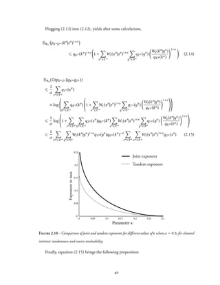
Therefore, the joint exponent is positive if
H(X|Z) − I( ˜Y; ˜K) > 0.
2.3.2.2 Comparison with Tandem Exponents
Figure 2.10 illustrates the gain of joint channel intrinsic randomness and source resolvability.
The problem of simulating a random process with a target distribution qKn from the output
of the channel W1 independently from its input corresponds to having Yn = Kn, W2 = idKn .
For qZn = qn
Z with qZ ∼ B(1/2), W1 = BSC(ω), and qKn = qn
K with qK ∼ B(κ) the joint
exponent becomes
Ecir
j (κ,ω) = max
α∈[0,1]
Ecir
j (α,κ,ω), (2.21)
where
Ecir
j (α,κ,ω) = − log ω1+α
+ (1 − ω)1+α
− log κ1−α
+ (1 − κ)1−α
. (2.22)
The separate approach consists in achieving the desired result in two distinct and indepen-
dent steps:
1. The DMCW1 is first used to extract an intermediate uniform random variable that takes
values in 1, 2nR (channel intrinsic randomness);
2. The uniform random variable is then used to generate the desired target process qKn
(source resolvability).
The exponents for these steps are derived as special cases of the joint exponent.
• For channel intrinsic randomness, the exponent to optimize is
E1(α,qZ ,W1,R) = − log
∑
z∈Z
qZ (z)
∑
x∈X
W1(x|z)1+α
− αR, (2.23)
which consists in taking Er (α, 2−nR,idK) = αR in the joint exponent.
• Similarly, for source resolvability, the exponent to optimize is
E2(α,qK,R) = αR − log
∑
kn ∈Kn
qKn (kn
)1−α
. (2.24)
42

Although there is no claim of optimality behind this result, note that these exponents are close
to the best exponents obtained by Hayashi [41] for variational distance. A slight improvement
of the exponents can be obtained in some cases, as shown by Watanabe [102].
Exponentinnats
Rate of the uniform intermediary process
Joint exponent
CIR exponent
Source resolvability exponent
……
Figure 2.11 – Determining the tandem exponent as the intersection of CIR and source resolvability exponents
and comparison with the joint exponent for κ = 0.2 and ω = 0.3.
As illustrated in Figure 2.11, the tandem exponent corresponds to the intersection of the
functions
R → max
α∈[0,1]
E1(α,qZ ,W1,R),
and R → max
α∈[0,1]
E2(α,qK,R).
In general, this intersection is below the optimal value of the joint exponent.
2.3.3 Converse
The following proposition presents a converse result for the joint scheme.
Proposition 2.32 For any DMC (Z,W1,X) and any DMSs (Z,pZ ) and (Y,qY ), joint chan-
nel intrinsic randomness and source resolvability requires
H(X|Z) ⩾ H( ˜Y) . ♢
43

Proof Assume that joint channel intrinsic randomness and source resolvability is possible. For
any ϵ > 0, there exists a mapping φn such that D(pYnZn ∥qKnqZn ) ⩽ ϵ. Using [26, Lemma
2.7] and Pinsker’s inequality gives the counterparts of Fano’s equality in traditional source and
channel coding.
• Since D(pYn ∥qYn ) ⩽ δ(ϵ), then
1
n
|H(Yn
) − H( ˜Yn
)| ⩽ δ(ϵ),
where δ(ϵ) denotes an arbitrary function of ϵ going to 0 with ϵ.
• Since D(pYnZn ∥pYnqZn ) ⩽ δ(ϵ),
1
n
I(Yn
;Zn
) ⩽ δ(ϵ).
Therefore,
H( ˜Y)
(a)
=
1
n
H( ˜Yn
)
(b)
⩽
1
n
H(Yn
) + δ(ϵ)
=
1
n
H(Yn
|Zn
) +
1
n
I(Yn
;Zn
) + δ(ϵ)
(c)
⩽
1
n
H(Yn
|Zn
) + δ(ϵ)
(d)
⩽
1
n
H(Xn
|Zn
) + δ(ϵ)
(e)
⩽ H(X|Z) + δ(ϵ). (2.25)
Steps (a) and (e) follow since the source is memoryless, (b) arises from the continuity of the
entropy rate, (c) from of the near independence of Yn and Zn, and (d) from the data processing
inequality since Yn is a function of Xn.
Proposition 2.33 For any DMC (Z,W1,X), any DMS (Z,pZ ) and (Y,qY ), and any ad-
ditive noise channel (Y,W2, K), joint channel intrinsic randomness and channel resolvability
requires
H(X|Z) ⩾ I( ˜Y; ˜K). ♢
44

Proof If the DMC (Y,W2, K) is an additive channel, then ˜K = ˜Y + E, where E is some
additive noise independent of the input ˜Y. In this case,
I( ˜Y; ˜K)
(∗)
=
1
n
I( ˜Yn
; ˜Kn
) =
1
n
H( ˜Kn
) −
1
n
H( ˜Kn
| ˜Yn
)
⩽
1
n
H(Kn
) −
1
n
H(En
) + δ(ϵ)
=
1
n
H(Kn
) −
1
n
H(Kn
|Yn
) + δ(ϵ)
=
1
n
I(Kn
;Yn
) + δ(ϵ)
⩽
1
n
H(Yn
) + δ(ϵ). (2.26)
Step (∗) comes from the memoryless nature of the source and channel. Following the same
steps as in the proof of Lemma 2.32 gives 1
n H(Yn) ⩽ H(X|Z) + δ(ϵ).
2.3.4 Discussion
If the channels are not memoryless, the analysis with the KL divergence does not carry over.
Nevertheless, to obtain asymptotical results in the general case, one may use variational distance
by replacing the criterion (2.3.1) by
lim
n→∞
V(pKnZn ,qKnqZn ) = 0. (2.27)
Using [38], the following sufficient condition obtained with a separate approach ensures the
existence of an encoding mapping φn:
p-liminf
n→∞
1
n
H(Xn
|Zn
) > p-limsup
n→∞
1
n
I( ˜Yn
; ˜Kn
), (2.28)
where H(Xn|Zn), and I( ˜Yn; ˜Kn) are defined as
H(Xn
|Zn
) ≜ log
1
pXn|Zn (Xn|Zn)
and I( ˜Yn
; ˜Kn
) ≜ log
W2( ˜Kn| ˜Yn)
qK( ˜Kn)
,
and
p-limsup
n→∞
Ξn ≜ inf
{
ξ lim
n→∞
P(Ξn > ξ) = 0
}
p-limsup
n→∞
Ξn ≜ sup
{
ξ lim
n→∞
P(Ξn < ξ) = 0
}
45

for an arbitrary sequence of random variable {Ξn}∞
n=1 [39]. Note that, for a memoryless process,
p-liminf
n→∞
1
n
H(Xn
|Zn
) = H(Xn
|Zn
) , and p-limsup
n→∞
1
n
I( ˜Yn
; ˜Kn
) = I( ˜Yn
; ˜Kn
)). (2.29)
A matching converse when W2 = idK can be found in [13].
Appendix 7.1 briefly provides some details of the construction of practical codes with polar
codes [7].
46

CHAPTER 3
THE TWO-WAY WIRETAP CHANNEL¹
The wiretap channel is limited to some particular aspects of a multi-user scheme, but does not
take into account cooperation, jamming, and feedback as means to increase secure communica-
tion rates. The two-way wiretap channel, in which users communicate over a noisy bidirectional
channel while an eavesdropper observes interfering signals, combines all the effects present with
multiple users because users have the possibility of cooperating while simultaneously jamming
the eavesdropper. This model was first investigated by Tekin and Yener [92, 93] who showed
that jamming with noise or controlled interference between codewords could provide secrecy
gains. However, this strategy, called cooperative jamming, does not exploit feedback. It was
later shown by He Yener [46] and Bloch [12] that strategies based on the feedback can per-
form strictly better than cooperative jamming alone. Recently, El Gamal et al. [28] proposed
an achievable region for the two-way wiretap channel combining cooperative jamming and a
secret-key exchange mechanism to transfer secure rate between users.
From a practical perspective, the two-way wiretap channel captures some of the limitations
of real systems because all communications are intrinsically rate-limited. The two-way wire-
tap channel also generalizes many models; for instance, the works of Amariucai and Wei [3],
Gündüz et al. [37], and Lai et al. [59] are special cases that focus on secure communication
for one user only. Similarly, the model of Ardestanizadeh et al. [5] is a two-way wiretap chan-
nel in which one of the links is confidential and unheard by the eavesdropper. Many works
on secret-key agreement with rate-limited public communication can be analyzed within this
framework [24, 103] as well.
This chapter extends existing results in several directions: it is possible to design powerful
coding schemes by partially decoupling the feedback and the interference and by relying on the
¹Parts of the material in this chapter have appeared in [76]: Pierrot, A. J., Bloch, M. R., “Strongly Secure
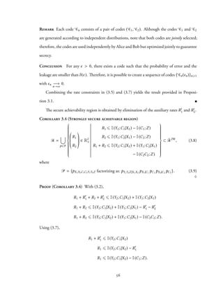
Communications Over the Two-Way Wiretap Channel”. In: IEEE Transactions on Information Forensics and
Security 6.3 (Sept. 2011), pp. 595–605. ©IEEE 2011.
47

strategies presented in Section 1.3: cooperative jamming, secret-key exchange and secret-key
generation.
Strong secrecy results, which require the eavesdropper to obtain a negligible amount of in-
formation instead of a negligible rate of information, exploit the concept of channel resolvabil-
ity [11, 38–40, 90] to analyze cooperative jamming. Channel resolvability provides a concep-
tually convenient interpretation of cooperative jamming, which allows analyzing what happens
when transmitting beyond the capacity of the eavesdropper’s channel.
The outline of this chapter is as follows. Section 3.1 introduces the definitions pertaining
to the two-way wiretap channel and a wiretap code. Section 3.2 presents a region of strongly
secure rates achievable with cooperative jamming based on channel resolvability. This first step
yields a result similar to what Tekin and Yener [92, Theorem 2] obtained for weak secrecy. In
Section 3.3, the region is improved by introducing the secret-key exchange mechanism pro-
posed in [28, 46]. The region is further extended by performing secret-key generation from a
source induced by the noise used in cooperative jamming. Finally, Section 3.4 illustrates the
achievable region in the Gaussian case.
3.1 Problem Statement
The problem of secure communication over a two-way wiretap channel is illustrated in Fig-
ure 3.1, in which:
• a legitimate user called Alice (or transmitter 1) sends message M1 and estimates M2;
• another legitimate user called Bob (or transmitter 2) sends message M2 and estimates M1;
• an eavesdropper called Eve observes Zn.
The channel is supposed to be full-duplex, which means Alice and Bob communicate simultane-
ously over the channel. This assumption is relevant for some communication systems; however,
it may be hard to realize in practice and many experimental communication systems operate
with half-duplex, potentially yielding lower rates.
48

Definition 20 A two-way wiretap channel, denoted by
(
X1,X2, Y1, Y2,Z, pYn
1 Yn
2 Zn|Xn
1 Xn
2 n⩾1
)
,
consists of two arbitrary input alphabets X1 and X2, three arbitrary output alphabets Y1, Y2
and Z, and a sequence of transition probabilities pYn
1 Yn
2 Zn|Xn
1 Xn
2 n⩾1 such that:
∀n ∈ N∗
, ∀ xn
1,xn
2 ∈ Xn
1 × Xn
2 ,
∑
yn
1 ∈Yn
1
∑
yn
2 ∈Yn
2
∑
zn ∈Zn
pYn
1 Yn
2 Zn|Xn
1 Xn
2
yn
1,yn
2,zn
|xn
1,xn
2 = 1. (3.1)
♢
Alice Bob
Eve
M1 ˆM1
ˆM2 M2
Xn
1
Xn
2
Zn
CODECCODEC
Two-Way Wiretap
Channel
Y n
1
Y n
2
pY n
1 Y n
2 Z n|X n
1 X n
2
Figure 3.1 – Communication over a two-way wiretap channel.
The subsequent analysis is limited to a memoryless wiretap channel, but this approach gen-
eralizes in part to arbitrary channels using information spectrum methods [38].
Definition 21 A memoryless two-way wiretap channel, denoted by
X1,X2, Y1, Y2,Z,pY1Y2Z|X1X2
,
is a two-way wiretap channel for which:
∀ xn
1,xn
2,yn
1,yn
2,zn
∈ Xn
1 × Xn
2 × Yn
1 × Yn
2 × Zn
,
pYn
1 Yn
2 Zn|Xn
1 Xn
2
yn
1,yn
2,zn
|xn
1,xn
2 =
n∏
i=1
pY1Y2Z|X1X2
(
y(i)
1 ,y(i)
2 ,z(i)
|x(i)
1 ,x(i)
2
)
. ♢
A code for the two-way wiretap channel is formally defined as follows.
49

Definition 22 A 2nR1, 2nR2,n two-way wiretap channel code Cn consists of:
1. Two message alphabets: M1 = 1, 2nR1 and M2 = 1, 2nR2 .
2. Two local sources of randomness R1,pR1 and R2,pR2 independent of the channel and
messages.
3. Two sets of encoding functions that map a message and past channel observations to a
channel input symbol:
• n encoding functions for transmitter 1:
∀i ∈ 1,n , f (i)
1 : M1 × Yi−1
1 × R1 → X1;
• n encoding functions for transmitter 2:
∀i ∈ 1,n , f (i)
2 : M2 × Yi−1
2 × R2 → X2.
4. Two decoding functions that map channel observations to a message or an error symbol
“ ?”:
• д1 : Yn
1 × M1 × R1 → M2 ∪ {?};
• д2 : Yn
2 × M2 × R2 → M1 ∪ {?}.
The performance of a code Cn is assessed in terms of the following quantities:
• the probability of error:
Pe( Cn) ≜ P (M1, M2) ( ˆM1, ˆM2)| Cn ;
• the information leakage to the eavesdropper:
L( Cn) ≜ I(Zn
; M1M2| Cn). ♢
50

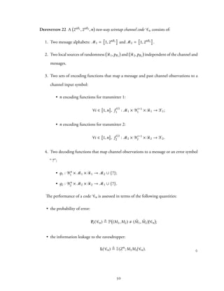
Definition 23 A rate pair (R1,R2) is achievable for a two-way wiretap channel if there exists
a sequence of codes { Cn}n⩾1 meeting the reliability and strong secrecy constraints:
• lim
n→∞
Pe( Cn) = 0 (reliability);
• lim
n→∞
L( Cn) = 0 (strong secrecy). ♢
Definition 24 The strong secrecy capacity region ¯R2W is defined as:
¯R2W
≜ cl ({(R1,R2) : (R1,R2) is achievable}) ,
whereas R2W denotes the weak secrecy capacity region. ♢
It is rather difficult to obtain a closed-form expression for the entire region of achievable rate
pairs (R1,R2). In principle, the coding scheme in Definition 22 could simultaneously exploit
the interference of transmitted signals at the eavesdropper’s terminal and feedback. To obtain
some insight, it is simpler to partially decouple these two effects.
• First, the interference penalizes the eavesdropper and increases secure communication
rates. The interference can be of two types: interference between codewords or jamming
with noise.
• Next, the feedback allows to increase the secrecy rate by means of key exchange and key
generation. With secret-key exchange, one user sacrifices part of its secure communica-
tion rate to exchange a secret-key, whereas, with secret-key generation, both users exploit
channel randomness to distill keys. Those keys are then used to encrypt messages with a
one-time pad.
3.2 Resolvability-Based Cooperative Jamming
3.2.1 Cooperative Jamming
A natural attempt to increase secure communication rates consists in jamming Eve with noise,
in order to decrease her signal-to-noise ratio. This strategy, called cooperative jamming [62],
forces one user to stop transmitting information to jam the eavesdropper. To overcome this
51

limitation, Alice and Bob can use codewords whose interference also has a detrimental effect
on Eve without sacrificing as much information rate. This scheme is called coded cooperative
jamming and was introduced by Tekin and Yener [92, 93]. It is possible to combine both
strategies and have Alice and Bob perform coded cooperative jamming while simultaneously
jamming the eavesdropper with noise. Simultaneous cooperative jamming can be implemented
by prefixing an artificial discrete memoryless channel (DMC) before the two-way wiretap chan-
nel (TWWTC) and sending codewords through the concatenated channels. This technique is
therefore called prefixing in [28].
Note that cooperative jamming does not exploit feedback, which corresponds to using only
two encoding functions f
(1)
1 and f
(1)
2 in Definition 22. Using cooperative jamming is then
equivalent to studying the simplified channel model illustrated in Figure 3.2, in which the
eavesdropper observes the output of a multiple-access channel.
Alice
Eve
M1
ˆM1
ˆM2
M2
Xn
1
Xn
2
Zn
ENC Two-Way
Wiretap
Channel
Y n
1
Y n
2
pY n
1 Y n
2 Z n|X n
1 X n
2
ENC
DEC
DEC
Bob
Figure 3.2 – Communication over a two-way wiretap channel without feedback.
3.2.2 Achievable Region
A first achievable region can be derived using the notion of channel resolvability, where uni-
formly distributed auxiliary messages M′
1 ∈ M′
1 ≜ 1, 2nR′
1 and M′
2 ∈ M′
2 ≜ 1, 2nR′
2 re-
spectively play the role of the sources of randomness R1,pR1 and R2,pR2 . Proposition 3.1
provides the region for rates (R1,R2,R′
1,R′
2).
52

Proposition 3.1
R = Proj
R1,R2
∪
p∈P



R1
R2
R′
1
R′
2
∈ R4
+
R1 + R′
1 ⩽ I(Y2;C1|X2)
R2 + R′
2 ⩽ I(Y1;C2|X1)
R′
1 + R′
2 ⩾ I(C1C2;Z)
R′
1 ⩾ I(C1;Z)
R′
2 ⩾ I(C2;Z)



⊂ ¯R2W
, (3.2)
where ProjR1,R2
is the projection on the plane of rates (R1,R2) and
P = {pX1X2C1C2Y1Y2Z factorizing as: pY1Y2Z|X1X2
pX1|C1
pC1 pX2|C2
pC2 }. (3.3)
♢
Remark A similar result has been independently established by Yassaee and Aref [108] using a
related technique based on approximation of output statistics. However, their proof only holds
for discrete memoryless channels because it involves strongly typical sequences. The following
proof relies on Steinberg’s results [90], which hold for Gaussian memoryless channels.
Proof Two types of transmitted messages are considered to introduce randomness. First, the
main messages must be transmitted between Alice and Bob reliably and securely with respect
to Eve. Second, the auxiliary messages are used to perform coded cooperative jamming and
introduce randomness to mislead the eavesdropper. Although auxiliary messages do not carry
information by themselves, Alice and Bob must decode them reliably. The scheme also includes
prefixing DMCs to perform simultaneous cooperative jamming.
The proof uses a random coding argument with fixed distributions pC1 , pC2 , pX1|C1
, and
pX2|C2
and a fixed ϵ > 0.
Code creation The code consists of randomly generated codewords with encoding and
decoding functions.
• Code generation: Generate 2nR1 2nR′
1 i.i.d. sequences cn
1(µ1) with µ1 = (i, j) ∈ M1 ×
M′
1 according topC1 , and 2nR2 2nR′
2 i.i.d. sequencescn
2(µ2) with µ2 = (i, j) ∈ M2 ×M′
2
according to pC2 . Here, i represents the index of the main message and j the index of the
53

auxiliary message. The random variable Cn represents the generated code, and Cn one of
its realizations.
• Encoding: If Alice wants to send µ1 ∈ M1 × M′
1, she computes cn
1 (µ1) and transmits xn
1
obtained by sending cn
1 through a DMC with transition probability pX1|C1
.
Similarly, if Bob wants to send µ2 ∈ M2 × M′
2, he computes cn
2 (µ2) and transmits xn
2
obtained by sending cn
2 through a DMC with transition probability pX2|C2
.
The DMCs with transition probability pX1|C1
and pX2|C2
are prefix channels used for si-
multaneous cooperative jamming to confuse the eavesdropper.
• Decoding: the decoder is a typical set decoder.
For simplicity, let An
1,ϵ ≜ An
ϵ (X1,C2,Y1) and An
2,ϵ ≜ An
ϵ (X2,C1,Y2).
If yn
1 is received by Alice, she selects ˆµ2 such that xn
1,cn
2 (ˆµ2) ,yn
1 ∈ An
1,ϵ. If such a tuple
exists and is unique, output ˆµ2, otherwise declare an error (ˆµ2 =?).
Similarly, if yn
2 is received by Bob, he selects ˆµ1 such that xn
2,cn
1 (ˆµ1) ,yn
2 ∈ An
2,ϵ. If such
a tuple exists and is unique, output ˆµ1, otherwise declare an error (ˆµ1 =?).
Probability of error analysis The probability of error is defined as
Pe( Cn)≜P (M1, M2, M′
1, M′
2) ( ˆM1, ˆM2, ˆM′
1, ˆM′
2) Cn . (3.4)
The following lemma provides conditions on rates such that this probability of error goes
to zero as n goes to infinity.
Lemma 3.2 (Probability of error) For ϵ > 0,



R1 + R′
1 < I(Y2;C1|X2)
R2 + R′
2 < I(Y1;C2|X1)
⇒ lim
n→∞
E(Pe(Cn)) ⩽ δ(ϵ). (3.5)
♢
Proof See Appendix 7.3.1 on page 128.
54

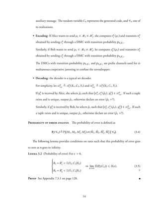
Remark Lemma 3.2 provides conditions for reliable communication regardless of the eaves-
dropper, which is intuitive because reliability only depends on what is happening between the
two legitimate users. However, this differs from the proof in [92], in which additional reliability
constraints that depend on the eavesdropper are introduced to compute the leakage.
Leakage analysis The leakage is defined as
L( Cn) ≜ I(Zn
; M1M2| Cn). (3.6)
Lemma 3.3 (Leakage) For ϵ > 0,



R′
1 + R′
2 > I(C1C2;Z)
R′
1 > I(C1;Z)
R′
2 > I(C2;Z)
⇒ lim
n→∞
E(L(Cn)) ⩽ δ(ϵ). (3.7)
♢
Remark Interpreting this result requires to precisely understand the role of auxiliary messages
M′
1 and M′
2. These messages replace the sources of randomness and Lemma 3.3 offers lower
bounds on the rates of these auxiliary messages. This result is also intuitive: more random-
ness must be introduced in the encoding process to prevent Eve from recovering the messages.
Lemma 3.3 demonstrates that there exist minimum values of the rates that allow zero asymp-
totic leakage.
It is important to remember that, because of the constraints imposed by Lemma 3.2, in-
creasing auxiliary message rates reduces the amount of information one can transmit through
the channel.
Code selection Lemma 2.23 (“Selection Lemma”) proves the existence of a specific se-
quence of codes { Cn}n⩾1 such that
lim
n→∞
Pe( Cn) ⩽ δ(ϵ) and lim
n→∞
L( Cn) ⩽ δ(ϵ).
55

Remark Each code Cn consists of a pair of codes ( C1, C2). Although the codes C1 and C2
are generated according to independent distributions, note that both codes are jointly selected;
therefore, the codes are used independently by Alice and Bob but optimized jointly to guarantee
secrecy.
Conclusion For any ϵ > 0, there exists a code such that the probability of error and the
leakage are smaller than δ(ϵ). Therefore, it is possible to create a sequence of codes { Cn(ϵn)}n⩾1
with ϵn −→
n→∞
0.
Combining the rate constraints in (3.5) and (3.7) yields the result provided in Proposi-
tion 3.1.
The secure achievability region is obtained by elimination of the auxiliary rates R′
1 and R′
2.
Corollary 3.4 (Strongly secure achievable region)
R =
∪
p∈P



R1
R2
∈ R2
+
R1 ⩽ I(Y2;C1|X2) − I(C1;Z)
R2 ⩽ I(Y1;C2|X1) − I(C2;Z)
R1 + R2 ⩽ I(Y2;C1|X2) + I(Y1;C2|X1)
− I(C2C2;Z)



⊂ ¯R2W
, (3.8)
where
P = {pX1X2C1C2Y1Y2Z factorizing as: pY1Y2Z|X1X2
pX1|C1
pC1 pX2|C2
pC2 }. (3.9)
♢
Proof (Corollary 3.4) With (3.2),
R1 + R′
1 + R2 + R′
2 ⩽ I(Y2;C1|X2) + I(Y1;C2|X1)
R1 + R2 ⩽ I(Y2;C1|X2) + I(Y1;C2|X1) − R′
1 − R′
2
R1 + R2 ⩽ I(Y2;C1|X2) + I(Y1;C2|X1) − I(C2C2;Z).
Using (3.7),
R1 + R′
1 ⩽ I(Y2;C1|X2)
R1 ⩽ I(Y2;C1|X2) − R′
1
R1 ⩽ I(Y2;C1|X2) − I(C1;Z).
56

Similarly, R2 ⩽ I(Y1;C2|X1) − I(C2;Z).
0
R0
2
lim
n!1
L( Cn ) = 0I(C1C2;Z)
I(C2;Z |C1)
I(C2;Z)
I(C1;Z) I(C1;Z |C2) I(C1C2;Z) R0
1
MAC
Figure 3.3 – Constraints on R′
1 and R′
2 in (3.2).
The region described in (3.8) is identical to the one obtained by Tekin and Yener in [92,
93] for weak secrecy. However, a closer look at the proof shows that their result is obtained by
projecting the region R′ defined as:
R′
=
∪
p∈P



R1
R2
R′
1
R′
2
∈ R4
+
R1 + R′
1 ⩽ I(Y2;C1|X2)
R2 + R′
2 ⩽ I(Y1;C2|X1)
R′
1 + R′
2 = I(C1C2;Z)
R′
1 ⩽ I(C1;Z|C2)
R′
2 ⩽ I(C2;Z|C1)



. (3.10)
This region differs from 3.2 only for the constraints on auxiliary message rates (R′
1,R′
2). The
difference is illustrated in Figure 3.3, where the dark area corresponds to constraints (3.7) and
the light one to the constraints on (R′
1,R′
2) in (3.10). Note that the latter corresponds to the
achievable region of a Multiple-Access Channel (MAC). This is not surprising because the proof
of (3.10) relies explicitly on the analysis of the probability of error for the eavesdropper, who
57

obtains its signal through a virtual multiple-access channel as depicted in Figure 3.2. In contrast,
the present approach analyzes the secrecy constraint directly, which leads to lower bounds on
the auxiliary message rate required to confuse the eavesdropper. The projection of both regions
on the plane of rates (R1,R2) is the same because it corresponds to having the auxiliary message
rates on the diagonal edge, which is common to both. In terms of code structure, the approach
of Tekin and Yener consists in augmenting the number of auxiliary messages until the leakage
to the eavesdropper become negligible, which only happens on the slope of the MAC region.
The constraints directly yield a region with negligible leakage and the approach consists in
finding the minimum number of auxiliary messages needed to confuse the eavesdropper, thus
augmenting the number of secret messages to the maximum possible value.
3.3 Secret-Key Exchange and Secret-Key Generation
The results in the previous section exploit the benefits of coded cooperative jamming and si-
multaneous cooperative jamming but do not consider the possibility of feedback. In particular,
two mechanisms leverage feedback.
• First, the techniques presented in [46] and [28] allow transferring secret rate from one
user to the other.
• Next, the randomness introduced by cooperative jamming is used to induce a source to
distill secret-keys. Results for secret-key agreement with rate-limited public communi-
cation [24, 103] prove useful since information can be only exchanged through a rate-
limited channel.
3.3.1 Key Exchange
Key exchange takes place on top of the cooperative jamming scheme by splitting the main and
auxiliary messages into multiple parts. The sub-messages facilitate the exchange of a secret-key
using the secret channel and encrypt part of the public message. Because of the “secret rate
transfer,” the rates must be redefined accordingly.
58

Consider a code for cooperative jamming with secret message rates (R1,R2) and auxiliary
messages rates (R′
1,R′
2). For i ∈ {1, 2}, the main message Mi is split into two parts.
• A key, which is used for encryption by the other user Ki ∈ Ki = 1, 2nRk
i ; user i needs
to sacrifice a part of its secret message to transmit this key.
• A secret message Ms
i ∈ Ms
i = 1, 2nRs
i ; this part corresponds to the part of the secret
message user i does not sacrifice.
The auxiliary message M′
i is also split into two parts.
• An encrypted version Me
i ∈ Me
i = 1, 2nRe
i of a message M/e
i . Encryption is done with a
secret-key provided by the other user and a one-time pad to ensure perfect secrecy [35].
• An open message Mo
i ∈ Mo
i = 1, 2nRo
i ; this corresponds to the part of the message that
remains public and is still perfectly decipherable by the receiver.
By convention, if no secret-key is available Re
i = 0, otherwise, by construction, Re
1 ⩽ Rk
2,
Re
2 ⩽ Rk
1. Since Mi = Ki × Ms
i and M′
i = Me
i × Mo
i , the various rates relate as
R1 = Rs
1 + Rk
1, R2 = Rs
2 + Rk
2, R′
1 = Ro
1 + Re
1, and R′
2 = Ro
2 + Re
2. (3.11)
Although (R1,R2,R′
1,R′
2) still represents the rates provided by cooperative jamming, they
are no longer the rates of interest after the secret-key exchange. In fact, part of the auxiliary
message is encrypted while part of the secret message is sacrificed to exchange a key. Thus, the
rates to consider are the following:
• a pair of secret rates: ˜R1 = Rs
1 + Re
1 and ˜R2 = Rs
2 + Re
2;
• a pair of public rates: ˜R′
1 = Ro
1 and ˜R′
2 = Ro
2.
Remark Because the secret-key sent by one user cannot be used simultaneously by the other,
the secret-key exchange scheme must operate in several rounds. The secret-key comes from the
previous one, except in the first round where no secret-key is available. A code of length n is
59

used B times, giving a new code of length n′ = Bn; the first message does not use secret-key
exchange, but the next B − 1 do. If the communication rate for the first message is R∗, for the
other (B − 1 is R, and the overall rate is
¯R =
nR∗ + n(B − 1)R
nB
=
B→∞
R.
Thus, the first round incurs a negligible rate penalty as B goes to infinity.
For weak secrecy, the authors of [28] prove the following proposition:
Proposition 3.5 (El Gamal et al.)
RF
=
∪
p∈P



R1
R2
R′
1
R′
2
∈ R4
+
R1 ⩽ I(Y2;C1|X2)
R2 ⩽ I(Y1;C2|X1)
R1 + R2 ⩽ I(Y2;C1|X2) + I(Y1;C2|X1)
− I(C2C2;Z)



⊆ R2W
, (3.12)
where:
P = {pX1X2C1C2Y1Y2Z factorizing as: pY1Y2ZX1X2 pX1|C1
pC1 pX2|C2
pC2 }. (3.13)
♢
Based on Section 3.2, this result also holds for strong secrecy: RF ⊂ ¯R2W.
Remark Comparing (3.8) and (3.12) proves that secret-key exchange improves the individual
bounds on R1 and R2, but not the bound on the sum-rate. Individual bounds on R1 and
R2 correspond to the capacity of the channel between the two users and cannot be improved;
therefore, any improvement in the region should modify the sum-rate constraint.
3.3.2 Key Generation from Induced Source
Key exchange requires sacrificing part of the secret rate of one user. In addition, the channel
randomness introduced for simultaneous cooperative jamming can be used to extract secret-
keys. Although users must exchange additional messages to agree on a common secret-key,
secret-key generation only comes at the expense of public message rate.
The next section focuses on the Gaussian two-way wiretap channel and explicitly demon-
strates how cooperative jamming induces a discrete memoryless source that can be used to distill
60

a secret-key. The existence of this DMS is not obvious because the noise introduced by cooper-
ative jamming is already exploited to harm the eavesdropper. It is a priori unclear if it could be
used simultaneously as a source of common randomness for secret-key agreement. First, one
must clarify what knowledge of the eavesdropper needs to be considered to identify the DMS.
Let K be the secret-key to distill and let M1, M2, M′
1 and M′
2 be the secret and auxiliary messages
used in the cooperative jamming code. The secret-key and secret messages must be indepen-
dent and both must be hidden from the eavesdropper, that is, for ϵ > 0, I(M1M2K;Zn) ⩽ ϵ.
Notice that
I(M1M2K;Zn
) = I(M1M2;Zn
) + I(K;Zn
|M1M2)
= I(M1M2;Zn
) + I(K;Zn
M1M2). (3.14)
The term I(M1M2;Zn) can be smaller than ϵ/2 by construction of the cooperative jamming
code, which requires I(K;ZnM1M2) ⩽ ϵ/2; this means that the secret-key must be hidden from
an eavesdropper having access not only to the observation Zn but also to the secret messages
M1 and M2. Furthermore, note that
I(M1M2K;Zn
) = I(M1M2;Zn
) + I K;Zn
M1M2M′
1M′
2 − I K; M′
1M′
2|Zn
M1M2 . (3.15)
If the cooperative jamming code is chosen to provide the highest secrecy rate, the public message
rates must be chosen to lie on the boundary of the region in (3.8), for which [92, 93] shows
that H M′
1M′
2|ZnM1M2 ⩽ ϵ/2. In this case,
I(M1M2K;Zn
) ⩾ I(M1M2;Zn
) + I K;Zn
M1M2M′
1M′
2 −
ϵ
2
. (3.16)
In other words, the secret-key K must be kept secret from an eavesdropper observing not only
the channel output Zn, but also knowing the secret and auxiliary messages transmitted by the
legitimate users.
3.3.3 Achievable Region with Secret-Key Exchange and Secret-Key Generation
Adding secret-key exchange and secret-key generation primitives to the coding scheme creates
new dependencies between the random variables of the different blocks. Splitting the messages
61

also introduces additional rate constraints and increases the dimension of the achievable rate
region.
3.3.3.1 Fundamental Considerations
The results of Lemma 3.3 relies on resolvability results for the multiple-access channel by Stein-
berg [90]. However, this proof does not take into account several subtleties that appear when
secret-key exchange and secret-key generation are performed over the two-way wiretap channel:
• the auxiliary messages M′
1 and M′
2 are no longer uniformly distributed;
• the eavesdropper does not have prior knowledge of the public messages sent;
• there exist dependencies between blocks since the secret-key is used across different blocks.
Non-uniform auxiliary messages The proof of Lemma 3.3 relies on the assumption that
the auxiliary messages are uniformly distributed. Part of the auxiliary message is encrypted
with a secret-key that is almost uniform, while the other part is used for the public message
communication. Since both these sub-messages are not exactly uniform, Lemma 3.3 cannot be
used directly and needs to be extended for the case of non-uniform messages.
Rate-limited secret-key generation is similar to the Wyner-Ziv problem [27], in which two
users distill identical sequences from a correlated source by exchanging messages over a rate-
limited public channel. In a similar fashion, the codebook generation operates as follows:
• the observation ˜Xn is sent trough a virtual channel, whose transition probability pU |X is
controlled by Alice;²
• sequences Un are labeled with three indices F ∈ 1, 2nRf , K ∈ 1, 2nRk , C ∈ 1, 2nRc
independently and uniformly distributed.
Using results from Chapter 2, several results follows:
²The case where Bob is generating the secret-key is similar.
62

1. channel intrinsic randomness ensures that indices are uniform and independent of ˜Zn,
i.e. V pFKC ˜Zn ,uF uK uC p ˜Zn ⩽ ϵ, if
Rf + Rk + Rc < H(U | ˜Z); (3.17)
2. Slepian-Wolf coding guarantees that it is possible to reconstructU by observing ˜Yn know-
ing indices F and K, i.e. there is a decoding function д such that P U д( ˜Yn,C) ⩽ ϵ,
if
Rf + Rc > H(U | ˜Y); (3.18)
3. channel intrinsic randomness with respect to ˜Xn establishes that index C is independent
of ˜Xn, i.e V pC ˜Xn ,uC p ˜Xn ⩽ ϵ, if
Rc < H(U | ˜X). (3.19)
These three constraints imply Rf > I U ; ˜X = I U ; ˜Y . The philosophy behind this approach
is to design a code for the virtual source (U, ˜X, ˜Y, ˜Z) based on the random binning of U with
three indices. The index F represents the public message that will be exchanged over the rate-
limited public channel; the index K represents the secret-key generated by both parties. The
role of index C is less intuitive since it is used to select a code among all possible codes provided
by this procedure. The first and third constraints guarantees secrecy, the second guarantee
reliability.
The next step consists in showing that designing a code for the virtual source (U , ˜X, ˜Y, ˜Z) is
equivalent to designing a code for secret-key generation. The source joint probability is denoted
pU ˜X ˜Y ˜Z , while the original joint probability representing the problem of secret-key generation is
denoted ˜pU ˜X ˜Y ˜Z . Including the auxiliary indices the total joint probability for the virtual source
is
pU ˜Xn ˜Yn ˜ZnFKC(u,xn
,yn
,zn
, f ,k, C)
= pFKC|U (f ,k, C|u)pU | ˜Xn (u|xn
)p ˜Xn ˜Yn ˜Zn (xn
,yn
,zn
), (3.20)
63

where Φ, Ψ and ϒ represents the random encoding functions respectively giving indices F, K,
and C for a given U . Note that
pFKC|U (f ,k, C|u) = 1{Φ(u) = f , Ψ(u) = k, ϒ(u) = C}.
To show that the code previously designed works also for the problem of secret-key generation
with rate-limited public communications, it suffices to verify that pU ˜X ˜Y ˜Z is close to ˜pU ˜X ˜Y ˜Z .
V pU ˜Xn ˜Yn ˜Zn , ˜pU ˜Xn ˜Yn ˜Zn = V pU ˜X ˜Y ˜Z , ˜pU ˜Xn ˜Yn ˜Zn
= V
(
pU ˜XnFKC,uCpFK|U pU |C ˜Xnp ˜Xn
)
= V
(
pFK|U pU |C ˜XnpC ˜Xn ,uC pFK|U pU |C ˜Xnp ˜Xn
)
= V pC ˜Xn ,uC p ˜Xn ⩽ ϵ. (3.21)
The indexC needs to be eliminated so that the same code can be used for any source observation
with an argument similar to the selection lemma.
P U д( ˜Yn
,C) ⩽ ϵ =
2nRc
∑
C=1
P U д( ˜Yn
, C) C = C uC ( C)
= EI P U д( ˜Yn
,C) C ⩽ ϵ. (3.22)
Markov’s inequality implies PI P U д( ˜Yn,C) C > 2ϵ ⩽ 1/2, thus there exists a particular
codebook C0 such that P U д( ˜Yn, C0) ⩽ 2ϵ
This coding scheme also guarantees that the message F and the secret-key K are almost uni-
form in terms of variational distance. The following lemma extends lemma 3.3 when auxiliary
messages M′
1 and M′
2 are not exactly uniform.
Lemma 3.6 If the following three conditions
lim
n→∞
1
n
H2(M′
1, M′
2) > I(X1X2;Z), lim
n→∞
1
n
H2(M′
1) > I(X1;Z), and lim
n→∞
1
n
H2(M′
2) > I(X2;Z)
(3.23)
are satisfied, then
∃β > 0, ECn (V(pM1M2Zn ,pM1pM2pZn )) ⩽ 2−βn
. (3.24)
♢
64

The proof of this lemma also relies on resolvability arguments but does not directly pro-
vide constraints on the communication rate. Instead, this lemma yields three constraints on
the second order Rényi entropy of the auxiliary messages. For the encrypted message Me
i (for
i ∈ {1, 2}), the encryption is performed with a one-time pad by using a secret-key Ki. The secret-
key Ki corresponds to the index K presented above and obtained from the previous round of
communication is almost uniform, that is V pKi ,uKi ⩽ ϵ, where uKi is the uniform distri-
bution with same support as Ki. The encryption operation is Me
i ≜ M/e
i ⊕ Ki where M/e
i is
the part of the auxiliary messages that needs to be encrypted. Additionaly, qMe
i
represents the
distribution of the encrypted message when M/e
i is uniformly distributed. Since the encryption
is performed with a one-time pad qMe
i
≡ uKi . The triangular inequality yields
V
(
pMe
i
,uKi
)
⩽ V
(
pMe
i
,qMe
i
)
+ V
(
qMe
i
,uKi
)
≡0
. (3.25)
Using the data processing inequality for the variational distance,
V
(
pMe
i
,qMe
i
)
⩽ V pKi ,uKi ⩽ ϵ. (3.26)
Therefore V
(
pMe
i
,uKi
)
⩽ ϵ.
The remaining part of the auxiliary message corresponds to the open message Mo
i that is
used as a public channel for the secret-key generation. This message corresponds to the index
F in the scheme presented before, which is such that V
(
pMo
i
,uF
)
⩽ ϵ.
As for the total auxiliary message pM′
i
= pMo
i
pMe
i
, and since Mo
i and Me
i are independent,
then
V
(
pM′
i
,uM′
i
)
= V
(
pMo
i
pMe
i
,uMo
i
uKi
)
⩽ V
(
pMo
i
pMe
i
,pMo
i
uKi
)
− V
(
pMo
i
uKi ,uMo
i
uKi
)
= V
(
pMe
i
,uKi
)
− V
(
pMo
i
,uMo
i
)
⩽ 2ϵ (3.27)
65

Prior knowledge of the eavesdropper The constraint (3.17) incidentally guarantees
that the public messages exchanged for the reconciliation are independent of the eavesdropper’s
statistics.
Dependencies between random variable Secret-key exchange and secret-key generation
require passing messages through different blocks. This introduces additional dependencies
among the random variables that must be taken into account in the analysis. For the sake of
simplicity, suppose both Alice and Bob simultaneously distill and use a secret-key.
independent/dependent r.v.
A EBr.v. associated to Alice r.v. associated to Bob r.v. associated to Eve
dependence within/between step
B
BB
A
A
A
AA A
AB
B
E
A
B
BB
A
A
A
AA A
AB
B
E
A
Block i Block i+1
/ /
M2,i+1
M2,i
M0
2,i
M0
1,i
M0
1,i+1
M0
2,i+1
Ki Ki+1
Xn
1,i Xn
1,i+1
Xn
2,i+1Xn
2,i
M1,i M1,i+1Cn
1,i
Si Si+1
Pi+1Pi
Cn
2,i Cn
2,i+1
Cn
1,i+1
Zn
i Zn
i+1
Figure 3.4 – Dependence graph when secret-key generation is used over the two-way wiretap channel (Alice
generates/uses the secret-key).
Figure 3.4 illustrates the initial steps of secret-key generation, when Alice both generates
and uses the secret-key, and represents the dependencies between the different blocks. For the
secrecy analysis the following term must be upper bounded
I
(
M1,1:BM′
1,2:BM2,1:B;Zn
1:B
)
,
where B represents the total number of blocks. The following lemma bounds the increase in
information brought by the observation of Zi+1.
66

Lemma 3.7 Let i ∈ 1, B − 1 . Define Li ≜ I
(
M1,1:BM′
1,2:BM2,1:B;Zn
1:i
)
. We have
Li+1 − Li ⩽ δn(ϵ). (3.28)
♢
Proof See Appendix 7.3.4 on page 137. This proof is given when Alice both generates and
uses the secret-key, but the result still holds for the three other configurations.
We then have
L1 = I
(
M1,1:BM′
1,2:BM2,1:B;Zn
1
)
= I M1,1M2,1;Zn
1 + I
(
M1,2:BM′
1,2:BM2,2:B;Zn
1 M1,1M2,1
)
⩽δn(ϵ) + I
(
M1,2:BM′
1,2:BM2,2:B;Zn
1 M1,1M2,1
)
⩽ δn(ϵ) + I
(
M1,2:BM′
1,2:BM2,2:B;Zn
1 M1,1M2,1
)
(∗)
= δn(ϵ),
where (∗) follows from independence of M1,2:BM′
1,2:BM2,2:B and the random variables of Block
1.
Hence, the strong secrecy over multiple blocks follows from Lemma 3.7 by remarking that
I
(
M1,1:BM′
1,2:BM2,1:B;Zn
1:B
)
= L1 +
B−1∑
i=1
(Li+1 − Li)
⩽ δn(ϵ) + (B − 1)(δn(ϵ))
= Bδn(ϵ).
3.3.3.2 Practical Considerations
Let one assume the existence of a DMS ( ˜X, ˜Y, ˜Z) independent of all other observations induced
by cooperative jamming. The statistics of the DMS depend both on channel statistics and the
code used for communications but does not need to be characterized completely.
67

First, note that substituting the rates defined in (5.17) in Proposition 3.1 provides a set of
constraints that achievable rates must satisfy:
Rs
1 + Rk
1 + Ro
1 + Re
1 ⩽ I(Y2;C1|X2) (3.29)
Rs
2 + Rk
2 + Ro
2 + Re
2 ⩽ I(Y1;C2|X1) (3.30)
Ro
1 + Re
1 + Ro
2 + Re
2 ⩾ I(C1C2;Z) (3.31)
Ro
1 + Re
1 ⩾ I(C1;Z) (3.32)
Ro
2 + Re
2 ⩾ I(C2;Z). (3.33)
Introducing the secret-key generation by splitting the codewords in multiple parts requires
to consider slightly different rates. For instance, the rates of interest for Alice become the
following.
• ˜Rs
1 = Rs
1 since secret-key generation does not change anything for the secret message rate.
• ˜Rk
1 = Rk
1 since secret-key generation does not change anything for the secret-key rate used
for secret-key exchange.
• ˜Ro
1 = Ro
1 − ¯R
p
1 − ¯Re
1. A part ¯R
p
1 of the open message rate is used for secret-key generation
while a part ¯Re
1 is used to transmit an encrypted message with that same key. Notice that
the constraint Ro
1 ⩾ ¯R
p
1 + ¯Re
1 must be satisfied.
• ˜Re
1 = Re
1 + ¯Re
1, thus increasing the encrypted message rate thanks to the secret-key gener-
ation mechanism.
Alice’s total secure communication rate is then ˜Rs
1 + ˜Re
1. Bob modifies his rates in a similar way.
Even if the DMS was characterized exactly, the secret-key capacity of a source with rate-
limited public communication is not known. Therefore, one may consider a suboptimal secret-
key agreement strategy in which a single user sacrifices a fraction ¯Rp of its open message rate for
communication and a single user uses the secret-key generated from the source for encryption.
68

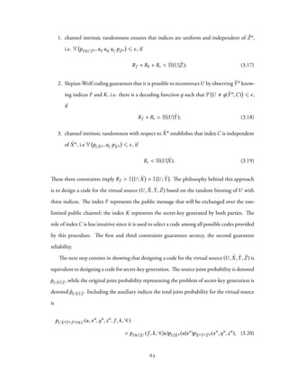
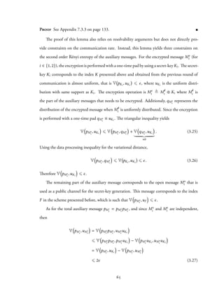
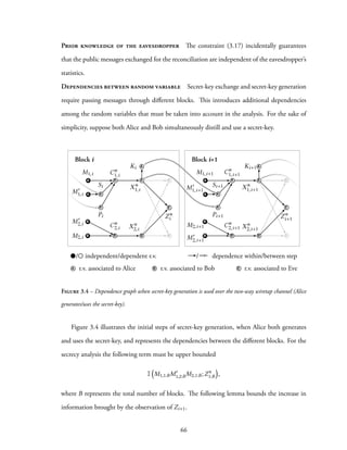
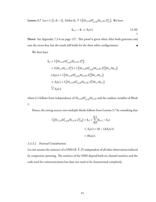
Table 3.1 – Additional constraints for secret-key generation.
Public Communication
Encryption Alice Bob
Alice: ¯Re
1 = ¯Rk
1, ¯Rk
2 = 0 ¯R
p
1 + ¯Rk
1 ⩽ Ro
1
¯R
p
1 ⩽ Ro
2, ¯Rk
1 ⩽ Ro
1
Bob: ¯Re
2 = ¯Rk
2, ¯Rk
1 = 0 ¯R
p
2 ⩽ Ro
1, ¯Rk
2 ⩽ Ro
2
¯R
p
2 + ¯Rk
2 ⩽ Ro
2
In this case, the optimal secret-key generation rate ¯Rk that can be distilled with rate-limited
public communication is known [24, Theorem 2.6]:
¯Rk
< I V ; ˜X|U − I V ; ˜Z|U ,
where the random variables U and V are such that U → V → ˜Y → ˜X ˜Z forms a Markov
chain and
I V ; ˜Y − I V ; ˜X ⩽ ¯Rp
.
Additional constraints on ¯Rp and ¯Rk exists, depending on which user performs public discus-
sion and which user encrypts a message. Specifically, there exist four possible configurations
presented in Table 3.1.
3.4 Gaussian Two-Way Wiretap Channel
This section focuses on the evaluation of some achievable regions based on the strategies devel-
oped in previous sections for the Gaussian two-way wiretap channel. The relationships between
inputs and outputs are



Yn
1 =
√
д1Xn
1 + Xn
2 + Nn
21,
Yn
2 = Xn
1 +
√
д2Xn
2 + Nn
12,
Zn =
√
h1Xn
1 +
√
h2Xn
2 + Nn
e .
(3.34)
In addition, the inputs are subject to the power constraints:
1
n
n∑
i=1
E
((
X(i)
1
)2
)
⩽ ρ1 and
1
n
n∑
i=1
E
((
X(i)
2
)2
)
⩽ ρ2.
69

The additive noises Nn
21, Nn
12, and Nn
e are supposed i.i.d. zero-mean unit-variance Gaussian
vectors. Cooperative jamming is performed by prefixing an additive white Gaussian noise
(AWGN) channel before each input of WTC2. This is equivalent to considering a modified
channel with inputs C1 and C2, with:
Xn
1 = Cn
1 + Nn
11 and Xn
2 = Cn
2 + Nn
22, (3.35)
where Nn
11 ∼ N(0, ρn
1In) and Nn
22 ∼ N(0, ρn
2In) correspond to the noise introduced by users to
realize cooperative jamming. For ρn
1 ⩽ ρ1 and ρn
2 ⩽ ρ2, the modified power constraints are
1
n
n∑
i=1
E
((
C(i)
k
)2
)
⩽ ρk − ρn
k = ρc
k, k = 1, 2.
With minor modifications of the proof presented in Section 3.2 to account for the power con-
straints, an achievable region for the Gaussian two-way wiretap channel can be obtained by
substituting the random variables C1 ∼ N(0, ρc
1) and C2 ∼ N(0, ρc
2) in the bounds obtained
earlier.
3.4.1 Randomness Source Extraction
Key extraction requires an explicit characterization of the DMS induced by cooperative jam-
ming. Define:



˜X1= N11, ˜Y1 = ˜X2 + N21,
˜X2= N22, ˜Y2 = ˜X1 + N12,
˜Z =
√
h1 ˜X1 +
√
h2 ˜X2 + Ne.
(3.36)
Proposition 3.8 The triple ( ˜X, ˜Y, ˜Z) with ˜X = ( ˜X1, ˜Y1) and ˜Y = ( ˜X2, ˜Y2) is an independent
DMS that can be used for secret-key generation. Alice, Bob and Eve observe the components
˜X, ˜Y, and ˜Z, respectively. ♢
Proof Since Alice generates the noise N11, she obtains ˜X1 directly. She also observes the
channel output Yn
1 = Cn
2 + Nn
22 + Nn
21 +
√
д1 Xn
1 ; since she knows Xn
1 and can decode Cn
2 with
high probability, she can obtain ˜Y1. Similarly, Bob can obtain ˜X2 and ˜Y2.
Eve observes the channel output Zn =
√
h1 Xn
1 +
√
h2 Xn
2 + Nn
e and, as discussed in Section 3.3,
70

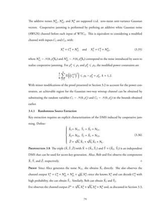
she obtains Cn
1 and Cn
2 as side-information. Therefore, Eve can compute ˜Z, but one needs to
show that ˜Zn is a sufficient statistic for ˜Xn and ˜Yn given (Zn,Cn
1,Cn
2). This is the case since
H ˜Xn
, ˜Yn
|Zn
Cn
1Cn
2
(a)
= H ˜Xn
, ˜Yn
| ˜Zn
Cn
1Cn
2
(b)
= H ˜Xn
, ˜Yn
| ˜Zn
, (3.37)
because (a): ZC1C2 → ˜ZC1C2 is bijective and (b): ( ˜X, ˜Y, ˜Z) is independent of (C1,C2).
The DMS ( ˜X, ˜Y, ˜Z) is a vector source, for which there is no known closed-form expres-
sion for the secret-key capacity with rate-limited public-rate communication. However, if Al-
ice and Bob ignore one of their observations, the DMS reduces to a degraded scalar source.
By [103, Corollary 2], there exists a closed-form function f
f : Rp →
1
2
log
Var(Y|XZ)e−2Rp + Var(Y|Z)(1 − e−2Rp )
Var(Y|XZ)
, (3.38)
which relates the public communication rate to the secret-key generation rates.
• If Alice ignores ˜Y1 and Bob ignores ˜X2, ˜Y2 → ˜X1 → ˜Z: if Bob sends public messages at
rate ¯Rp, Alice and Bob can distill a secret-key at rate ¯Rk, such that ¯Rk ⩽ f
(
¯Rp,p ˜Y2 ˜X1 ˜Z
)
.
• If Bob ignores ˜Y2 and Alice ignores ˜X1, ˜Y1 → ˜X2 → ˜Z: if Alice sends public messages at
rate ¯Rp, Alice and Bob can distill a secret-key at rate ¯Rk, such that ¯Rk ⩽ f
(
¯Rp,p ˜Y1 ˜X2 ˜Z
)
.
With the explicit characterization of the DMS induced by cooperative jamming and the
function f , it is possible to compute new achievable rates for the strategy described in Sec-
tion 3.3. Although there is no known closed-form expression for the resulting region ¯RK, it is
possible to prove that the region strictly includes the region ¯RF in Proposition 3.5 strengthened
for strong secrecy.
Proposition 3.9 Consider ¯RF, ¯RK, and ¯R2W defined as before. In general: ¯RF ⊆ ¯RK ⊆
¯R2W. There exist channels such that ¯RF ⊂ ¯RK.
Proof The first statement follows directly from the definition of the secret-key generation
strategy in Section 3.3. For the second statement, consider the example of a channel for which:
0 < ρ1 <
h2 − 1
h1
and 0 < ρ2 <
h1 − 1
h2
.
71

In this case I(C1;Y2|X2) < I(C1;Z) and I(C2;Y1|X1) < I(C2;Z), thus the region ¯RF is empty.
However, since the power constraints are non-zero, a fraction of the power can be used to induce
a DMS while still maintaining a positive auxiliary message rate. By [103, Theorem 3], it is
possible to obtain a non-zero secret-key rate and, therefore, a non-zero secure communication
rate.
Remark Although the proof yields ¯RF ⊂ ¯RK by exhibiting a dummy example, the numerical
results in the next section clearly confirm improvements in various cases.
3.4.2 Results
ρ1 = 1 ρ2 = 100 h1 = 1 h2 = 0.1 д1 = д2 = 1
0.0 0.1 0.2 0.3 0.4 0.5
¯RK ¯RF ¯R ¯Rout
Secret rate (bits/channel use)R1
Secretrate(bits/channeluse)R2
0.0
0.1
0.2
0.4
0.6
0.3
0.5
Figure 3.5 – Region evaluation for д1 = д2 = 1, ρ1 = 1, ρ2 = 100, h1 = 1, h2 = 0.1.
The first situation considers that the secret-key generation provides little gain because coop-
erative jamming leaves little room for improvement. Figure 3.5 illustrates the achievable region
with simultaneous cooperative jamming and secret-key exchange ¯RF, and the achievable region
that also includes secret-key generation ¯RK obtained for ρ1 = 1, ρ2 = 100, h1 = 1, h2 = 0.1,
and д1 = д2 = 1. The upper left corner of the region corresponds to a situation in which Alice
uses all her power to jam (ρn
1 = ρ1) while Bob uses all his power to transmit (ρc
2 = ρ2). A
secret-key can be extracted from the source induced by Alice; however, since h1 = 10, Eve’s
72

source observation is highly correlated to Alice’s, which severely limits secret-key rates. The
upper right corner of the region corresponds to a situation in which both Alice and Bob use
their entire power to transmit (i.e., ρc
1 = ρ1 and ρc
2 = ρ2) and, therefore, no source is induced.
For comparison, the figure also illustrates the region ¯R obtained using secret-key generation
alone (no cooperative jamming). Although this strategy is clearly suboptimal, note that there
exist practical coding schemes for secret-key generation over Gaussian channels; therefore, the
region ¯R provides an estimate of rates achievable with current codes. These results can be com-
pared to the best-known outer region ¯Rout for the two-way wiretap channel computed by He
and Yener [43].
ρ1 = 1 ρ2 = 100 h1 = 1 h2 = 0.1 д1 = д2 = 1
ρ1 = ρ2 = 1 h1 = h2 = 1.5 д1 = д2 = 1
0.0 0.1 0.2 0.3 0.4 0.5
0.0
0.5
1.0
2.0
3.0
1.5
2.5
Figure 3.6 – Region evaluation for д1 = д2 = 1, ρ1 = ρ2 = 1, h1 = h2 = 1.5.
Figure 3.6 illustrates the regions ¯RF and ¯RK obtained for ρ1 = ρ2 = 1, h1 = h2 = 1.5,
and д1 = д2 = 1. This corresponds to a situation in which Eve obtains a better observation
than either Alice or Bob and in which Alice and Bob have little power available. In such a case,
secret-key generation provides a significant improvement.
Finally, Figure 3.7 illustrates the region ¯RF and ¯RK obtained for ρ1 = ρ2 = 0.9, h1 = h2 = 10,
and д1 = д2 = 1. In this case ¯RF = ∅, but secret-key generation is possible.
73

д1 = д2 = 1 ¯ = ∅
ρ1 = ρ2 = 0.9 h1 = h2 = 10 д1 = д2 = 1
N1 N2
Z = h1X1 + h2X2 + Ne ,
0.0 0.1 0.2 0.3 0.4
0.0
0.1
0.2
0.4
0.3
0.5
Figure 3.7 – Region evaluation for ρ1 = ρ2 = 0.9, h1 = h2 = 10, д1 = д2 = 1.
3.5 Conclusion and Discussion
This chapter provides an achievable region of strongly secure rates based on strategies that par-
tially decouple the use of interference and feedback for secrecy. The coded cooperative strategy
exploits the interference, while secret-key exchange and secret-key generation exploit the feed-
back. This combined approach shows significant improvements in the Gaussian case. More
recently, several results have considered new models of multi-user communications. For in-
stance in [46], the authors consider both full-duplex communications and half-duplex commu-
nications with an untrusted relay. For the first model, not exploiting the feedback induces an
unbounded loss in secrecy rate in some cases. For the latter model, the penalty is negligible if
the relay power is unlimited. The authors derive an achievable region with a simple cooperative
jamming scheme that does not exploit feedback while showing near-optimal performances.
74

CHAPTER 4
EXPERIMENTAL ASPECTS OF SECRET-KEY GENERATION¹
As seen in the previous chapters, physical-layer security promises new ways of providing secrecy
through the utilization of the intrinsic randomness present in any communication medium,
such as noise and interferences. Although the theory behind physical-layer security has been
extensively studied, designing and implementing a physical-layer security system in a wireless
environment remains a challenge. Without additional experimental validation, there is a risk
that the models considered in theoretical works may be fairly disconnected from real systems
since they rely on assumptions that cannot be met in a real wireless setting.
Table 4.1 – Literature comparison.
Reference Experiments Statistics Security Analysis
[100, 101, 111] No
Postulated or N/A
Non information-theoretic[19, 63, 98] Simulations
[52, 72, 79, 80]
Yes
[61]
I(X;Z) = 0 because of
decorrelation
[49, 99, 105, 109]
Estimated from
experimental
measurements
Asymptotic
information-theoretic
Proposed Yes
Estimated from
experimental
measurements
Finite Length
As summarized in Table 4.1, several works have already experimentally investigated the
generation of secret-keys from wireless channels. In fact, the gains of wireless channels pro-
vide a natural source of randomness, for which reciprocity guarantees that legitimate users
obtain strongly correlated channel observations, while diversity ensures that the observations of
¹Parts of the material in this chapter have appeared in [75]: Pierrot, A. J., Chou, R. A., Bloch, M. R., “Experi-
mental Aspects of Secret Key Generation in Indoor Wireless Environments”. In: Proceedings of the 14th Workshop
on Signal Processing Advances in Wireless Communications (SPAWC). June 2013, pp. 669–673. ©IEEE 2013.
75

a third-party eavesdropper disclose little information about the legitimate users’ measurements.
However, while these works are often motivated by an information-theoretic formulation, the
information-theoretic model is not fully developed. In particular, common assumptions about
the eavesdropper’s statistics, such as the decorrelation of channel gains at distances larger than
half the wavelength, as well as the use of asymptotic values of secret-key generation, lead to over-
simplifications of the protocols and over-estimations of the achievable information-theoretic
secret-key rates. Consequently, while canonical theoretical models of wireless channels have
proved incredibly useful to design reliable communication systems, their use for the design of
secret-key generation systems requires more care. Similarly, checking that generated keys pass
statistical tests [6]–[9], which have been primarily designed for mathematical cryptography
and only verify some desirable statistical property of the key, does not guarantee information-
theoretic secrecy.
The objective of this chapter is to investigate the practical effect of eavesdropper’s statistics by
implementing a secret-key generation system from wireless channel gain with software-defined
radios, and by carrying out a careful information-theoretic analysis. The weakness of previously
reported system lies in the modeling of the source of randomness, but not in the operation of the
subsequent protocol; therefore, this chapter does not attempt to develop a complete secret-key
generation system. The results obtained in this chapter yields the following conclusions:
1. assuming that the eavesdropper does not get any information because of decorrelation
with distance is not exact in a real wireless system;
2. the existence of a correlated eavesdropper’s observation makes the evaluation of the finite-
length secret-key rates much more intricate.
Section 4.1 recalls the basic principles of secret-key generation from channel variations,
with the underlying mathematical formalism and assumptions. Section 4.2 describes the exper-
imental setup used to induce a source of randomness by leveraging the variations of the channel
76

gains. Section 4.3 assesses the robustness of the scheme regarding the diversity assumption. Sec-
tion 4.4 presents an achievable secret-key rate with a finite number of samples, which is then
evaluated with the experimental measurements. Finally, Section 4.5 provides some conclusions
and discussions regarding the possible limitations for the design of practical physical-layer se-
curity systems with an example of potential application.
4.1 Key Generation from Channel Variations
This section formalizes a generic process that extracts a source of randomness from the channel
and then describes how the secret-key is generated from such a source.
4.1.1 Secret-Key Generation Strategy
4.1.1.1 Randomness in Wireless Channels
In a wireless channel with impulse response h(t), the signal i(t) emitted by a terminal and the
corresponding signal o(t) received at another are related as
o(t) = (h ∗ i)(t) + w(t).
The thermal noise w(t) appears at the receivers because of the thermal agitation in the
electronic circuits. This noise is highly random, unpredictable, and has a short coherence time.
It is not suitable for secret-key generation since there is no correlation among the thermal noises
at different terminals.
The impulse response h(t) of a wireless channel between two terminals results from the
reflections and attenuations underwent by the transmitted signal along different paths. This
chapter focuses on narrowband channels with approximately 1 MHz bandwidth, for which the
received signal is essentially a delayed version of the original one attenuated by a random com-
plex gain G(t) exp(ȷφ(t)). This complex gain accounts for the aggregated effect of attenuation
and phase change of each path; note that reciprocity guarantees that the gain GAB(t) between
two points A and B is the same as the gain GBA(t) between the points B and A. The coherence
time during which the gain G(t) and the phase φ(t) remain constant scales approximately as
Tc ≈ λ/v, where λ is the wavelength and v is the characteristic speed of the environment. For
77

instance, in the experimental setup described later, the objects around the receiver move at
about one meter per second, so that the coherence time is on the order of milliseconds for wire-
less communications at 2.5 GHz. It is easier to exploit the randomness of the channel gain G(t)
since precise measurements of the phase φ(t) require a precise synchronization of the terminals.
4.1.1.2 Randomness Extraction
Alice's terminal Bob's terminal
Eve's terminal
Legitimate Parties
Eavesdropper
Setting characteristics
Central frequency: 2.484 GHz
Bandwidth: 4 MHz
Switch period: 80 ms
hAB
hBA
hAE hBE
Figure 4.1 – Experimental testbed with software-defined radios.
Following common practice, and as illustrated in Figure 4.1, the channel gains between
the two legitimate terminals are measured in Time-Division-Duplex mode as follows. The first
terminal, Alice, sends a complex probe signal b(t) with unit energy, whose duration β is much
smaller than the coherence time Tc, so that the channel gain G remains almost constant over
the pulse duration. The second terminal, Bob, measures from the channel a delayed and faded
version ˜b(t) of b(t). Using his knowledge of the probe signal, Bobs matches ⃗b(t) = ˜b(t + Td)
and b(t) as
Td = argmaxτ (⃗b ∗ b)(τ). (4.1)
78

Then, Bob estimates the channel gain from Alice to Bob as
GAB =
√∫
β
⃗b(t)
2
dt, (4.2)
by measuring the energy of the delayed received probe signal. Simultaneously, an eavesdropper,
Eve, obtains a channel gain GAE. Alice estimates the channel gain GBA in a similar fashion from
Bob’s probe signal, which also provides Eve with a channel gain GBE in the process.
4.1.2 Mathematical Formalism
Once n measurements are performed, Alice, Bob, and Eve, effectively observe the components
of a noisy source (Xn YnZn,pXnYnZn ), in which Xn consists of n channel gains Gn
BA, Yn consists
of the channel gain Gn
AB, and Zn consists of both sequences Gn
AE and Gn
BE. A secret-key gener-
ation strategy Sn for the source (Xn YnZn,pXnYnZn ) with unlimited public communications
consists of the following operations.
• Reconciliation: Alice transmits a public message F over the public authenticated channel,
which allows Bob to construct an estimate ˆXn of Xn from Yn and F.
• Privacy amplification: Alice chooses a function G uniformly at random in a family of
universal2 hash functions, which is disclosed to all parties. Alice then computes G(Xn) ∈
K while Bob computes G( ˆXn). Setting K ≜ 1, 2nR , R is called the secret-key rate.
In principle, Alice and Bob could interactively exchange messages, but this strategy is restricted
to unidirectional operation. The secret-key generation strategy Sn must ensure the following:
1. reliability, measured with the probability of disagreement
Pd(Sn) ≜ P(K ˆK|Sn);
2. (strong) secrecy, measured by the leakage
L(Sn) ≜ I(K;Zn
F|Sn);
79

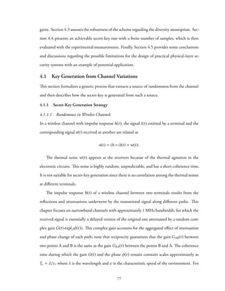
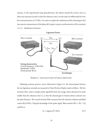
3. (strong) uniformity, measured by
U(Sn) ≜ log 2nR
− H(K|Sn).
Computing the aforementioned metrics requires the knowledge of source statistics, including
that of the eavesdropper.
A secret-key rate R ≜ 1
n log |K| is achievable if the three above metrics tend to zero as n
goes to infinity, and the supremum of achievable secret-key rates is called the secret-key capacity
Cs. Most recent works have focused on the calculation of Cs, which is an asymptotic limit
obtained for infinitely many realizations of the source; in contrast, the analysis conducted in
Section 4.4 focuses on a finite length behavior that only requires L(Sn) and U(Sn) to be small,
but non-zero.
4.1.3 Assumptions behind the secret-key generation model
The secrecy guaranteed by a secret-key generation strategy rely on three common assumptions.
Availability of an authenticated public channel of unlimited capacity This as-
sumption is not unreasonable if one aims at generating low secret-key rates for which the
amount of public communication is negligible compared to the channel capacity. If one explic-
itly introduces a rate limitation, reconciliation with vector quantization can be used [21, 24]
without fundamentally affecting the operation of the secret-key agreement strategy.
Existence of enough randomness Mobility in the environment is required to ensure that
wireless channel gains have enough entropy. Mobility results from the movements of objects
around the terminals or the terminals themselves; in indoor wireless environments, this channel
gains experience variability as soon as people move around the communication terminals.
Knowledge of eavesdropper’s statistics In an information-theoretic secret-key gener-
ation model, one requires the knowledge of the statistical dependencies between Eve’s obser-
vations and the legitimate users’ to assess the secrecy of the keys. Unfortunately, there exists
no indirect way to estimate these statistical dependencies of the eavesdropper without perform-
ing measurements at Eve’s terminal position. In addition, as pointed out in [52], the statistics
80

should not be influenced by the eavesdropper to prevent the induction of artificial, determin-
istic, and predictable variations of the channel parameters. In principle, if Eve only has partial
control of the environment, any uncontrolled movement would suffice to induce variations she
cannot predict. This assumption might be even more easily satisfied in wideband and MIMO
systems since it would require more advanced capabilities from the attacker.
The knowledge of the eavesdropper’s statistics is the most crucial assumption for the proper
operation of a secret-key generation system. This could be avoided by operating in a quantum
setting, e.g. [104], but such systems are only efficiently implemented in optics. In the classical
wireless setting, the assumption is often circumvented by assuming that there exists enough
diversity in the environment, so that one can either assume that I(GAB;GAEGBE) = 0 meaning
the eavesdropper’s observations are completely independent of the legitimate users’, or, at least,
that I(GAB;GAEGBE) is upper bounded. However, it is crucial to precisely assess the conditions
under which the diversity assumption may hold, so as to define situations in which secret keys
can be safely generated. Moreover, it is considerably easier to analyze secrecy assuming that
I(GAB;GAEGBE) = 0 and that the eavesdropper only observes public communication. Privacy
amplification and reconciliation are simply linked using the result of Cachin and Maurer [18],
and counting the number of bits disclosed during privacy amplification is sufficient to establish
the final key length. In contrast, when I(GAB;GAEGBE) 0, the final secret key length depends
on the eavesdropper’s statistics and one must factor in the effect of statistical deviations from
the mean when using a finite number of samples n.
4.2 Experimental Source Induction
This section describes the experimental setup and the procedure to characterize the statistics of
the wireless channel gains. The gain measurements are reported for a source that is induced
using a communication chain representative of a typical wireless system.
81

4.2.1 Setup Description
The system features three USRPs (see Appendix 7.2 for more details) with XCVR2450 daugh-
terboards that operate in the 2.5 GHz and 5 GHz bands, typically used for Wi-Fi communi-
cations. However, the bandwidth is not wide enough (8 MHz maximum) to allow for actual
Wi-Fi communications according to the IEEE standards, which would require over 20 MHz of
bandwidth. Consequently, the reported secret-key rate is likely to be much smaller than what
could be obtained on top of an IEEE802.11 transmission. RF signals are transmitted using
standard Wi-Fi antennas with a transmission power below 100 mW.
The experiments are conducted in two ordinary office rooms representative of an indoor
environment: one is the former Arcom wireless communication laboratory at Georgia Tech
Lorraine, and the other is a conference room. The choice of which room used for the experi-
ments was only motivated by convenience.
All radios are connected to a single computer that processes the transmission and reception
data stream. There is no external hardware synchronization between the terminals, and the
same configuration is used for all terminals, both in hardware and software. The first samples
of the data stream are used to overcome hardware discrepancies by scaling all measurements to
obtain the same received energy. After calibration, the scaling is kept constant through each
experiment since no significant drift was observed during acquisition.
4.2.2 Communication Chain
All experiments were conducted using the three-user setup represented in Figure 4.1. The mod-
ulation frequency is 2.484 GHz, which corresponds the 14th WLAN channel. This channel is
not used in for Wi-Fi communications and does not interfere with other Wi-Fi channels. Since
XCVR2450 daughterboards are limited to half-duplex operation, the channel gains cannot be
measured simultaneously. This limitation occurs in a majority of communication systems since
full-duplex communication requires complex hardware and software implementation [10]. To
circumvent the problem, the radios are continuously switching between the Rx and Tx modes.
Because of further hardware restrictions, the minimum half-duplex cycle time is limited to
82

Binary File
(Probe)
Mapping
Raised
Cosine
Filter
Gain USRP
BIT
1 bit
COMPLEX
14 bits
COMPLEX
14 bits
COMPLEX
14 bits
BINARY
{0,1}
BPSK
{-1,1}
Post
Processing
Channel
Gain
Estimation
AGCUSRP
COMPLEX
12 bits
COMPLEX
12 bits
COMPLEX
12 bits
PLL
COMPLEX
12 bits
Computed from the
probe signal
Transmission
Reception
Figure 4.2 – Communication chain for channel gain estimation.
80 ms. Consequently, motion in the environment is limited to 1 m.s-1 so that the channel gain
would not vary much between an Rx/Tx switch, thus maintaining channel reciprocity. If the
hardware allowed faster half-duplex cycle to capture faster fades, higher secret-key generation
rates would be achieved in a high mobility environment, but the security analysis would remain
essentially the same.
4.2.3 Characterization of Induced Source Statistics.
The estimation of the channel gains is performed using a probe message sent through the com-
munication chain described in Figure 4.2. The gain present in the transmission chain allows
power control and is kept constant throughout the entire duration of the experiment. Dur-
ing the reception, the USRP performs demodulation and analog-to-digital conversion. An
automatic gain controller (AGC) scales the received signal to match the optimal range of the
subsequent processing block. Note that it is tuned to be slow enough not to remove the gain
variations over the timescale of interest. Because the system operates at a high carrier frequency,
a phase-locked loop (PLL) is used to suppress any residual modulation resulting from minor dif-
ferences between modulation and demodulation frequencies. The demodulated signal is then
used to compute the transmission gain. Note that all parties know the probe signal and that the
83

0 1 2 3 4 5 6 7 8 9 10
0
1
2
3
Time (s)
NormalizedChannelGain(a.u.)
GAB GBA GAE GBE
Figure 4.3 – Channel gain measurements.
transmission chain behavior is entirely deterministic so that all users also know the shaped sig-
nal and can compute the channel gain. The probe signal, which is a fixed randomly-generated
sequence, is also used to synchronize the different radios in software.
A total of 500 gain measurement experiments were acquired, each lasting approximately
ten seconds. Alice and Bob’s terminals were separated by 1.5m and Eve’s terminal was approxi-
mately 1m away from both Alice and Bob. Figure 4.3 illustrates the evolution of the following
four channel gains: the channel gain GAB from Alice to Bob, its reverse GBA from Bob to Alice,
the channel gain GAE from Alice to Eve, and the channel gain GBE from Bob to Eve. It appears
that GAB closely follows GBA, confirming the existence of channel reciprocity. Eve’s channel
gains GAE and GBE are seemingly not related to the channel gains GAB and GBA, potentially
confirming the existence of channel diversity. According to Jake’s model, diversity should hold
as soon as Eve is farther from Alice and Bob than the coherence distance, which is ℓc = λ/2 ≈
6 cm, at 2.484 GHz. The next section analyzes diversity more precisely.
It is desirable to operate on a memoryless source of randomness to make the statistical char-
acterization tractable. Decimating the raw measurements in Fig. 4.3 is a way to remove the
84

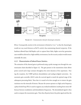
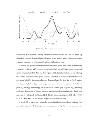
0 20 40 60 80 100
0
0.2
0.4
0.6
0.8
1
1.2
1.4
1.6
Sample delay ν
I(X0;Xν)(bits)
Figure 4.4 – Evolution of the self-correlation of channel gains.
time correlation by keeping a single sample per coherence interval; since the coherence time
is on the order of magnitude of λ/v, Tc should be on the order of one second. It is possible
to obtain a more precise characterization of the value of Tc with an estimation of the mutual
information I(X0;Xν ) between a sample X0 and the ν-th next sample Xν , obtained by viewing
each of the experimental time series as the realization of the same ergodic random process. The
lower I(X0;Xν ) is, the less dependent the samples are. To use more samples for the estimation,
the gains are supposed wide sense stationary, which was empirically confirmed by verifying that
the quantity I(X0;Xν ) remained the same for different choices of X0. Unless mentioned other-
wise, all information metrics are estimated with the technique presented in [73]. As illustrated
in Figure 4.4, the mutual information I(X0;Xν ) decays rapidly and vanishes after a dozen sam-
ples, corresponding to approximately one second, as expected. Operating on the down-sampled
measurements instead of the original measurements would result in a lower achievable secret-
key rate, which might seem an unnecessary simplification since it is possible to characterize
achievable secret-key rates for sources with memory [17, 19]. However, without an accurate
parametric model, the estimation of the statistics of a source with memory turns out to be a
much more difficult problem.
85

The final step is then to estimate the joint statistics pXYZ of the memoryless source, which
poses two challenges. First, one would in principle need to analyze the estimation error and
include it in the subsequent calculation of achievable key rates; the results presented in this
chapter do not take this into account and assume that the estimation is accurate enough to be
used as the true joint statistics. Second, the measurements only provide quantized measure-
ments XQ, YQ and ZQ of the true channel gains X, Y, and Z, respectively. The quantization of
X and Y is not critical since it reduces achievable secret-key rates by only affecting the reconcil-
iation step. However, the quantization of Z results in an underestimation of the eavesdropper’s
knowledge, therefore one should assume that the eavesdropper can keep Z continuous. Since it
is not possible to acquire a continuous-valued Z with the software-defined radios, the first step
consists in constructing a histogram corresponding to pXQYQZQ′ from the measured data, where
ZQ′ is a quantized version of Z. Then the histogram is interpolated with respect to ZQ′ to obtain
pXQYQZ . The raw data was acquired with a 14 bits resolution, which was further quantized to
obtain a 4-bit resolution for XQ and YQ, and a 6.5-bit resolution for ZQ′.
4.3 Statistics of the Channel Gain Observations
4.3.1 Empirical Gain Distribution
The histogram of the values of the source is represented Figure 4.5. In a wireless environment
with many diffractive and reflective objects, one can show that (see [94]) channel gains follow
a Rician distribution of the form
fR(r) =
2(K + 1)r
Ω
exp
(
−K −
(K + 1)r2
Ω
)
I0 2
√
K(K + 1)
Ω
r ,
with (K, Ω) ∈ R2
+.
The parameter K is the ratio between the line of sight energy transmission and the reflected
or diffracted paths energy. In this case, estimating the parameters K and Ω from the empirical
moments [2] yields the distribution in Figure 4.5.
The distribution fitting yields the following parameters K = 2,48 and Ω = 1. This value
for K confirms a strong line of sight between the two terminals. Regarding Ω, its small value
can be justified because of the small number of diffractive objects.
86

Normalized Gain (arb. unit)
Frequency(%)
0 1 20.5 1.5 2.5
3.0
6.0
1.5
4.5
0.0
Rician fit
Experimental
7.5
Figure 4.5 – Gain distribution
4.3.2 Robustness of the Diversity Assumption
Diversity is desirable to facilitate the generation of keys at a high rate so that the eavesdropper’s
observations are not correlated to legitimate users’. The ideal case would be a perfect statisti-
cal independence between these observations. However, even intuitively, it seems unlikely to
happen; for instance, if Eve is close to either Alice or Bob, she may be able to obtain a strongly
correlated observation of the channel gain. In an ideal case, the correlation would decay with
distance, but this also depends on the configuration of the objects populating the environment.
A series of measurements² was conducted in the building conference room to verify whether
diversity holds in a narrowband wireless setting. The room is about 40 square meters and is
furnished as illustrated in Figure 4.6. Experiments were conducted off-hours to avoid any
unwanted motion outside of the room. Two radios were placed in the middle of the room
on the conference table two meters apart. A third radio terminal represents the eavesdropper,
which was moved in the room across 60 possible positions. The channel gains GAB and GAE
obtained by Bob and Eve is then used to evaluate information leakage. These experiments only
²Acknowledgment: Alan Dong for his valuable help for those experiments.
87

involved one-way communications (Alice-to-Bob and Alice-to-Eve), thus avoiding the problem
of half-duplex operation and allowing to gather data at a faster pace. Each experiment lasted
one minute, yielding about 50,000 channels gain values at a 1 kHz sampling rate. The first
and last hundred of samples were removed to eliminate artifacts when starting and stopping
the radios.
The results of the measurement campaign are presented in Figures 4.6 and 4.7. Eve is placed
across the positions indicated by the black “+” marks, which correspond to a coarse square grid
of one meter and additional positions to cover interesting locations and the room borders. The
brightness represents the normalized secrecy-rate (for GAB = GBA) between the gains obtained
by Eve and those obtained by Bob, which is computed as
Normalized secrecy-rate ≜
I(GAB;GBA) − I(GAB;GAE)
I(GAB;GBA)
= 1 −
I(GAB;GAE)
H(GAB)
, (4.3)
where GAB and GAE are the channel gains measured by Bob and Eve, respectively. This nor-
malization compensates the entropy variations of the wireless channel gains across different
experiments. This quantity is close to one (white) when the gains are independent, and equal
to zero (black) when there is a one-to one mapping between GAB and GAE.
The first series of measurement, reported in Figure 4.6, is conducted without movement
and serves as a benchmark. In this situation, there is no fluctuation of the channel gains, except
those induced by the noise at the receivers’ terminals. Therefore, the quantity I(GAB;GAE) is
small since the receiver noise is independent from one radio to another. When Eve and Alice use
the same antenna, the darker spot comes from the electronic coupling between the terminals.
In a second series of measurements, represented in Figure 4.7, the operator is walking in
the upper left corner of the room. High correlations appear when Bob and Eve’s antennas are
huddled together, and a fast decay of this correlation with distance, with leaked information
reaching almost zero after a few centimeters. However, the leaked information increases again
further away, even reaching values as high as 10% in the upper left corner. Since this corner
88

5.47 m
6.71m
0%
100%
Normalizedsecrecy-rate
100%
96%
98%
94%
98%
Alice
Bob
Figure 4.6 – Normalized secrecy rate without motion.
was actually the area where the operator was moving during the experiment, it suggests that
measurements close to the motion source provide a better insight into the legitimate channel
fluctuations. Therefore, defining a simple zone of guaranteed secrecy for key generation is not
straightforward. From a security standpoint this proves that one cannot ignore the information
leaked to the eavesdropper when channel variations come from the motion in the environment.
It confirms that a secret-key generation must include a stage of privacy amplification to deal
with unforeseeable levels of leaked information.
89

5.47 m
6.71m
Motion
Zone
90%
95%
99%
100%
90%
97%
Alice
Bob
0%
100%
Normalizedsecrecy-rate
Figure 4.7 – Normalized secrecy rate with motion.
4.3.3 Environment Inﬂuence
The environment has a significant influence on the secret-key generation rate since the gain
fluctuations used as a source of randomness are induced by external motion. The number
of secret-key bits generated per second mainly depends on two factors: the entropy of the
channel gain value provided by the source and the number of samples provided by the source
per second. The latter depends on the coherence time of the channel since the decimation of
the gain measurements relies on this value.
90

The experimental testbed used to analyze the influence of the environment is slightly dif-
ferent from previous experiments and consist of two radios placed on a cart to estimate the
channel gain in one direction. The experiments were performed in the following situations:
1. the cart is moved in a hallway at a slow pace (about 2 km/h);
2. the cart is moved in a hallway at a normal pace (about 4 km/h);
3. the cart is moved in a hallway at a fast pace (about 6 km/h);
4. the cart is parked in the hallway with nobody moving around;
5. the cart is parked in the hallway between classes;
6. the cart is spun inside the building lobby;
7. the cart is parked outside;
8. the cart is moved outside at a fast pace (about 6 km/h);
9. one radio is shaken, while the other stays still.
The gain measurements are further filtered to remove the measurement noise and to solely
keep the gain fluctuations, using a running average filter with a span of 20 ms, which is much
lower than the typical time of the gain fluctuations for motions slower than 10 km/h.
Table 4.2 – Gain measurement entropy and secret-key rate upper bound in various situations.
Situation 1 2 3 4 5 6 7 8 9
Gain entropy (b.p.g.v.) 6.86 7.49 8.33 2.00 2.81 9.78 6.15 9.95 8.61
Coherence Time (ms) 510 328 181 18,904 9,474 322 4,230 57 148
Max secret-key rate (bit/sec) 13.4 22.8 46.0 0.11 0.30 30.4 1.45 175 58.1
Table 4.2 confirms that the gain entropy only depends on the presence of motion. The
gain entropy is limited to 12 bits, which is the resolution of the analog-to-digital converters.
The coherence time appears to be more sensitive to motion, which is what one would expect
91

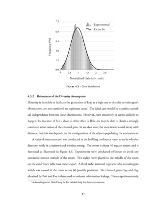
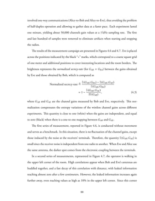
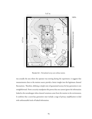
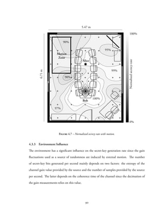
from the direct relationship between the coherence time and the velocity of moving objects in
the environment. This table also provides an upper bound on the secret-key bitrate by taking
the ratio of the gain entropy over the coherence time, even though this may be far from what
can be obtained considering the entire secret-key generation scheme with reconciliation and
privacy amplification. As expected, the secret-key rates are higher when there is more mobility
in the environment; bitrates are also higher in an outdoor environment, probably because the
experiments conducted in the hallway involved a limited number of scatterers.
4.4 Secret-Key Generation in the Finite Blocklength Regime
Once the statistics pXQYQZ of the source are characterized, one can easily compute asymptotic
achievable secret-key rates I XQ;YQ −I XQ;Z . However, these rates may be far too optimistic
when operating on a finite number of samples, and it is crucial to avoid overestimating the num-
ber of secret bits that one can effectively extract with reconciliation and privacy amplification.
The analysis in 4.4.1 is based on the detailed study of privacy amplification with continous
eavesdropper’s observation, which differs from the finite-length analysis in [95, 102] restricted
to discrete observations. The numerical results in 4.4.2 are also obtained for the memoryless
sourcepXQYQZ characterized experimentally in Section 4.2, and not from computer simulations.
The only approximation in this analysis is that the source statistics estimated in Section 4.2.3
correspond to the true statistics; the entire analysis in Section 4.4.1 is exact.
4.4.1 Finite-Length Analysis for a Continuous Observation Z
As stated in 4.2.3, the following finite-length analysis assumes that the eavesdropper’s observa-
tion Z is continuous and that the estimation of the statistics of the source made in Section 4.2.3
is accurate.
The finite key-length analysis relies on a sequential strategy [16, 67], in which the recon-
ciliation step is performed with error correction codes and the privacy amplification step is
performed with hash functions. However, since Z is continuous, it is not possible to directly
92

use previous approaches [9, 67], which are only valid for discrete random variables, or that can
only be extended to continuous random variables in an asymptotic regime [20, 21].³
The reconciliation protocol is performed on the quantized versions XQ and YQ of X and Y,
and Prec
e corresponds to the probability of error of the reconciliation step, while ℓrec represents
the number of information bits leaked during the process.
A lower bound on H(K|GZnF) is needed to determine the final secret-key length obtained
after privacy amplification with a hash function G chosen at random. This quantity represents
the uncertainty obtained by the eavesdropper with its own observation Zn, the knowledge of
G, and the public message F. The strategy Sn is also known by the eavesdropper, but is omitted
in the subsequent analysis to simplify the notation.
The goal is to bound the equivocation H(K|ZnFG). This section explains how to bound
this quantity as
k − δϵ(n) ⩽ H(K|Zn
FG) ⩽ k, (4.4)
where k represents the size of the output of the hash function G used to distill the key. The
finite length analysis consists in estimating k for a given n. Using the results in [102, Corollary
2] for privacy amplification, it follows that
E (V(pKZnFG,uKnpZnFG)) ⩽ 2ϵ +
1
2
√
2nR−Hϵ
∞
(
Xn
Q |ZnFG
)
. (4.5)
This expression involves the ϵ-smooth min-entropy of Xn
Q given the information available
at the eavesdropper’s terminal. This quantity cannot be directly evaluated, but relates to other
information theoretic metrics that can be estimated.
Lemma 4.1 Let S andU be two random variables and let r > 0. Then, with probability at least
1 − 2−r ,
Hϵ
∞ (S) − Hϵ
∞ (S|U = ¯u) ⩽ log |U| + r. (4.6)
♢
³Note that, in principle, it is possible to quantizeZ since by [78][32][23, Section 8.5][8, Lemma 2][21, Lemma
1.2], for any δ > 0, if a quantized version ZQ′ of Z is fine enough,
|I(K;AZ) − I K; FZQ′ | < δ.
93

4.4.2 Numerical Evaluation
The experiments provide four different channel measurements. Since both Alice and Bob trans-
mit probe signals, they can respectively obtain the channel gains GBA and GAB. Incidentally,
Eve can also estimate the channel gains GAE and GBE. The source of randomness is therefore
(X,Y,Z), where X = GBA, Y = GAB, and Z = (GAE,GBE).
GAB
GAB GBA
GBA
GBE
GBE
GAE
GAE
Figure 4.8 – Correlations between the different normalized channel gains.
Figure 4.8 illustrates how the channel gain measurements conducted in Section 4.2.3 are
correlated with each other. This figure shows that the channel gains GBA and GAB are strongly
correlated and confirms the hypothesis of reciprocity. The correlation is, however, not perfect,
thus justifying the reconciliation phase in the secret-key generation protocol. On the other
hand, there is no substantial correlation either between both Eve’s observations GAE and GBE,
or between Eve’s observations and the legitimate users’ observations. This second observation
confirms the hypothesis of diversity when Eve is not located near one of the antennas of the legit-
imate parties. Looking solely at the distributions of the channel gains yields similar conclusions
95

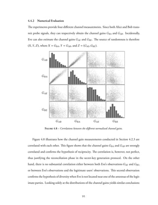
since GBA and GAB have similar distributions (reciprocity), while GAE and GBE have different
distributions due to the different path followed by the electromagnetic waves (diversity).
If the reconciliation protocol has an efficiency β ∈ [0, 1] (see [16]), then lrec = n(H(X) −
βI(X;Y)) bits are leaked to the eavesdropper. The best case scenario, obtained for β = 1, would
yield H(X|Y) bits leaked during the reconciliation step. Note that the value of β may change
depending on the blocklength n.
Asymptotically, it is known that the corresponding achievable secret-key rate is Rlow ≜
I(X;Y) − I(X;Z), which is a lower bound of the secret-key capacity Cs [66].
0 1 2 3 4 5
·104
0.3
0.4
0.5
0.6
0.7
0.8
0.9
1
Blocklength n
Ratioη
β = 1
β = 0.95
β = 0.90
β = 0.85
β = 0.80
Figure 4.9 – Ratio η, for U < 10−3 and L < 10−3.
The gap between the finite and the asymptotic regime is quantified using the ratio
η ≜
k/n
Rlow
,
where Rlow ≈ 1.46 bits is a known achievable rate, which is upper bounded by the secrecy
capacity Cs, which is such that Cs ⩽ I(X;Y|Z) ≈ 1.76 bits.
96

The main limitation of a secret-key generation scheme relying on channel variations is the
difficulty to clearly establish the conditions to provide secrecy without precise knowledge of the
eavesdropper’s statistics. The experiments show that there is no simple relationship between
the eavesdropper’s proximity and the correlation of its observations. Even worse, it appears that
if the eavesdropper induces motion, it might be able to obtain an accurate estimation of the
legitimate users’ own observations. This is consistent with the observations made in [52] when
the adversary controls the environment to induce a predictable channel behavior.
As already seen in [65, 109], there is also a strong relationship between the environment
mobility and the achievable secret-key rate. The secret-key generation scheme should account
for these variations to avoid extracting more randomness than possible. For instance, depending
on the degree of mobility of the environment, the coherence time will change and the length
of the secret-key should change accordingly.
Estimating the source statistics not only allows one to assess the security of the system,
but also to define the source induction functions and to select the hash function output size.
However, the estimation of the source statistics is a problem in itself, especially because the
eavesdropper’s observations are not available to legitimate users.
Finally, the achievable secret-key generation rate also depends on the blocklength. Thus a
lightweight scheme that operates with short codes will have much lower performances than a
scheme operating with infinitely long codes.
To increase secret-key generation rates, one possibility is to consider other channel para-
meters to obtain a source with more randomness. In theory, the channel phase is uniformly
distributed and may exhibit more entropy than the gain magnitude. However, designing a
secret-key generation scheme using the channel phase would be technically challenging and
would require complex synchronization between terminals.
To maintain a minimum level of secrecy regardless of the environment properties, it is
crucial to address the lack of eavesdropper channel state information (CSI) for the legitimate
97

users. For instance, one can obtain a significant advantage by using multiple antennas [20, 43,
99]. Again, this improvement would make the system more complex, and such choice would
depend on the final desired level of secrecy.
98

CHAPTER 5
PRACTICAL CODED COOPERATIVE JAMMING¹
Historically, coding theory has focused on designing codes that are good for reliability, but
not directly meant to do binning for the wiretap codes. However, the growing interest for
physical-layer security has spurred the development of new coding techniques for secrecy based
on powerful error-correcting codes, such as low-density parity-check (LDPC) codes and polar
codes.
The underlying ideas behind coding for secrecy, which are motivated by the analysis of the
wiretap channel by Wyner [107], are twofold. Randomness should be introduced to confuse the
eavesdropper by sending a random sequence along with the actual message and the codebook
should exhibit a binning structure. One approach [4] consists in employing two-edge LDPC
codes with a coset encoding technique in which the binning is controlled by the two-edge
structure. Another approach [54, 106] is to use punctured LDPC codes to create a nested linear
code structure. Both constructions exhibit performances close to the weak secrecy capacity
when employed with spatially coupled LDPC codes [4, 53, 57, 82]. A last approach consists
in exploiting polar codes to achieve the secrecy capacity as described in [22, 64] and references
therein. All these works open up new directions for the design of practical codes for secrecy.
This section presents a code construction based on punctured LDPC codes for the multiple-
access channel to perform coded cooperative jamming. This scheme guarantees weak secrecy
and its performances are analyzed for both classical and spatially coupled LDPC codes.
The outline of this chapter is as follows. Section 5.1 introduces and motivates the two-way
wiretap model considered in this chapter. Section 5.2 introduces spatially-coupled LDPC codes
for the multiple-access channel. Section 5.3 describes how to use SC-LDPC codes to provide
¹Parts of the material in this chapter have appeared in [77]: Pierrot, A. J., Bloch, M. R., “LDPC-Based Coded
Cooperative Jamming Codes”. In: Proceedings of the IEEE Information Theory Workshop. Lausanne, Switzerland,
Sept. 2012, pp. 462–466. ©IEEE 2012.
99

secrecy and assesses the performances of the proposed coding scheme. Section 5.4 concludes
this chapter and discusses some of the model assumptions.
5.1 Coded Cooperative Jamming for the Two-Way Wiretap Channel
5.1.1 General Model
CODEC
Xn
1
Xn
2
M1
ˆM2
ˆM1
Nn
1
Nn
2
Nn
e
M0
1 M0
2
Two-Way Wiretap
Channel
Legitimate
User 1
Legitimate
User 2
Eavesdropper
h1 h2
Y n
M2
CODEC
Figure 5.1 – Communications over the Gaussian two-way wiretap channel.
Consider a special case of the model presented in the previous section called the binary-
input memoryless Gaussian two-way wiretap channel, which is presented in Figure 5.1. N1 and
N2 represent the noise at legitimate users’ terminals. From the eavesdropper’s standpoint,
Z =
√
h1X1 +
√
h2X2 + Ne, (5.1)
where
• X1,X2 ∈ {−1, 1} are BPSK modulated symbols;
• + is the usual real number addition;
• Ne is a centered Gaussian noise with variance σ2 and independent of channel inputs; and
gains are unitary h1 = h2 = 1.
The hypothesis of equal-gained interferences may appear restrictive since this situation is
unlikely to naturally arise in a real wireless setting as shown in Section 5.4. However, one can
100

imagine a situation in which the eavesdropper is an honest-but-curious third user that also
communicates, but should not access some of the information exchanged over the network.
Since this user communicates over the network, it is possible to estimate its channel parameters
and to induce pure interferences at its terminal by appropriately scaling power.
This model neglects the interferences between codewords at the legitimate receivers’ termi-
nals since the interferences that occur between exchanged codewords may be canceled by the
knowledge of the transmitted sequences.
5.1.2 Erasure MAC
To make code design more tractable, the model is further simplified thanks to the following
lemma.
Lemma 5.1 Any memoryless q-input channel X,pY|X , Y (the output alphabet can be either
continuous or finite) is stochastically degraded with respect to the q-ary erasure channel with
erasure probability ϵ∗ defined as
pZ|X =



ϵ if Z =?
1 − ϵ if Z = X
0 otherwise
ϵ∗
≜
∫
Y
min
u∈ 0,q−1
pY|X (y|u)dy.
♢
Proof Let X,pZ|X ,Z be a q-ary erasure channel with erasure probability ϵ∗ {0, 1}:
pZ|X = ϵ∗
1{Z =?} + (1 − ϵ∗
)1{Z = X},
with X = 0,q − 1 and Z = X ∪ {?}. Now, define the channel Z,pY|Z , Y as follows
pY|Z (y|?) =
1
ϵ∗
min
u∈ 0,q−1
pY|X (y|u) , (5.2)
pY|Z (y|z) =
1
1 − ϵ∗
(
pY|X (y|z) − min
u∈ 0,q−1
pY|X (y|u)
)
, if z ∈ 0,q − 1 . (5.3)
101

For any (x,y) ∈ X × Y,
∑
z∈Z
pY|Z (y|z)pZ|X (z|x) = pY|Z (y|?)ϵ∗
+
∑
z∈ 0,q−1
pY|Z (y|z) (1 − ϵ∗
)1(z = x)
= min
u∈ 0,q−1
pY|X (y|u) + pY|X (y|x) − min
u∈ 0,q−1
pY|X (y|u)
= pY|X (y|x) . (5.4)
In particular, this shows that the channel ({−2, 0, 2},pY|X1+X2
, R) is stochastically degraded
with respect to a ternary erasure channel. This observation allows to further simplify the model
by considering the erasure multiple-access channel defined as follows
Z =



X1 + X2 with probability 1 − ϵ
? with probability ϵ
, (5.5)
where ϵ = 2Q (2/σ) . This channel is not strictly equivalent to the initial model, but the data
processing inequality ensures that the information received by the eavesdropper from the actual
channel is smaller than the information it would obtain from the output of the erasure multiple-
access channel.
The achievable communication rates (R1,R2) for such an erasure channel must satisfy
R1 ⩽ I(X1;Y|X2) = 1 − ϵ,
R2 ⩽ I(X2;Y|X1) = 1 − ϵ,
R1 + R2 ⩽ I(X1,X2;Y) ≜ Csum = 3(1 − ϵ)/2, (5.6)
which is obtained with uniform input symbols. Equivalently, the maximum erasure rate cor-
rectable by codes of rates R1 and R2 is
ϵShannon = min (1 − R1, 1 − R2, 1 − 2/3(R1 + R2)) . (5.7)
5.1.3 Leakage Analysis
Codes for the MAC are used in the following way to obtain secrecy for the two-way wiretap
channel.
102

• Xn
1 (resp. Xn
2 ) corresponds to the codeword sent by legitimate user 1 (resp. user 2) over
the channel and obtained from secure message M1 ∈ 1, 2nR1 (resp. M2 ∈ 1, 2nR2 )
randomly encoded with an auxiliary message M′
1 ∈ 1, 2nR′
1 (resp. M′
2 ∈ 1, 2nR′
2 ).
• Zn corresponds to the observation of an eavesdropper at the output of the erasure multiple-
access channel. This eavesdropper must not get any information about the secure mes-
sages M1 and M2.
The secrecy metric is chosen to be the leakage rate (weak secrecy criterion); for a given code
Cn, ensuring secrecy requires
lim
n→∞
L ( Cn) = 0, with L( Cn) ≜
1
n
I(Zn
; M1, M2| Cn). (5.8)
It can be shown that (for simplicity, the conditioning on Cn is dropped)
nL( Cn) = I(M1M2;Zn
)
= I M1M2M′
1M′
2;Zn
− I M′
1M′
2;Zn
|M1M2
= I Xn
1 Xn
2 ;Zn
+ I M1M2;Zn
|Xn
1 Xn
2
=0 (M1M2→Xn
1 Xn
2 →Zn)
−I Xn
1 Xn
2 ;Zn
|M1M2
= I Xn
1 Xn
2 ;Zn
− H M′
1M′
2|M1M2 + H M′
1M′
2|M1M2Zn
= I Xn
1 Xn
2 ;Zn
− H M′
1M′
2 + H M′
1M′
2|M1M2Zn
⩽ nCsum − n(R′
1 + R′
2) + H M′
1M′
2|M1M2Zn
. (5.9)
Hence, to provide secrecy, the code rates R′
1 and R′
2 must compensate Csum and minimize
H M′
1M′
2|M1M2Zn . This last condition corresponds to considering a virtual receiver capable
of decoding (M′
1, M′
2) from (M1, M2,Zn). For code that allows this with an error probability
P′
e, Fano’s inequality ensures
H M′
1M′
2|M1M2Zn
⩽ Hb P′
e + nP′
e(R′
1 + R′
2).
5.2 LDPC Codes for the MAC
The previous chapters have shown that coded cooperative jamming is one of the mechanisms
for providing secrecy in a multi-user scheme. However, the analysis only provides some insight
103

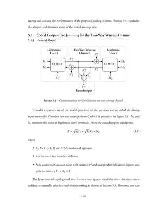
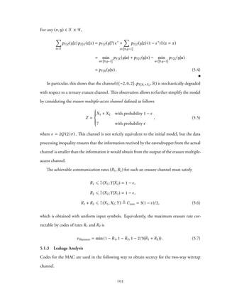
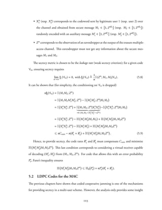
into the general structure of the code without providing any efficiently implementable codes.
This section introduces spatially coupled low-density parity-check codes (SC-LDPC) for the MAC
as presented in [56].
5.2.1 Spatially-Coupled LDPC Codes
Spatially coupled LDPC codes, SC-LDPC for short, are based on the standard LDPC codes
that aim at increasing the belief propagation (BP) threshold by coupling individual LDPC
codes. This construction, which has been introduced by Felström and Zigangirov [53] and fur-
ther analyzed by Kudekar et al. [57], is capacity-achieving for the binary erasure channel. The
capacity-based approach for secrecy relies on the use of good codes for reliability. This subsec-
tion presents the basic construction of SC-LDPC codes to clarify the mathematical definitions
and properties of such ensembles. These codes also exhibit better floors than classical irregular
LDPC codes and better finite-length performances than polar codes.
5.2.1.1 The (l,r, L) Ensemble
The construction of the (l,r, L) ensemble [57] consists in repeating and coupling several LDPC
protographs, which are based on small regular (l,r) LDPC codes.
Definition 25 A protograph P = (V, C, E) is a bipartite graph that consists of a set of
variable nodes V, a set of check nodes C, and a set of edges E. Each edge e ∈ E connects a
variable node ve ∈ V to a check node ce ∈ C. A variable node and a check node are connected
by multiple edges. ♢
For the construction of the (l,r, L) ensemble [57] where r = kl and l is odd, the pro-
tograph PSC consists of one check node and k variable nodes, where each variable node is
connected to the unique check node by r edges. For example, Figure 5.2 depicts the proto-
graph of a standard (3,6)-regular ensemble. The protograph is then repeated 2L + 1 times and
then for each check node:
• keep only one edge and disconnect the l − 1 remaining ones;
104

... ...
... ...
Check Node Variable Node
Figure 5.2 – Spatially-coupled LDPC ensemble construction.
• connect a pair of edges to the first adjacent check nodes, a pair to the second adjacent
variable nodes, etc.;
• if there is no available adjacent check node, remove the edge.
This construction based on protograph can be generalized for cases where r is not a multiple
of l, but l is still odd.
1. Take 2L + 1 sets of M variable nodes vi,j with i ∈ −L, L and j ∈ 1, M . The total
number of variable nodes is therefore M(2L + 1).
2. Take 2(L + ˆl) + 1 sets of Ml/r check nodes ci,j with i ∈ −L − ˆl, L + ˆl , ˆl = (l − 1)/2,
and j ∈ 1, Ml/r .
3. At each position i ∈ −L− ˆl, L+ ˆl , there are exactly Ml check node sockets. Randomly
connect the check nodes to the variable nodes vi,· with i ∈ i − ˆl,i + ˆl .
5.2.1.2 The (l, r, L,w) Ensemble
The (l, r, L) ensemble is rather complicated to analyze and can be simplified by introducing
another level of randomization in the construction. The construction consist of
1. 2L + 1 sets of M variable nodes vi,j with i ∈ −L, L and j ∈ 1, M ;
105

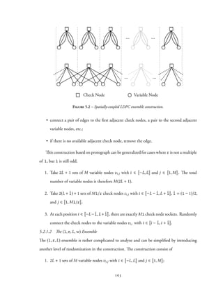
2. an infinity of candidate check nodes ci,j with i ∈ N, ˆl = (l − 1)/2, and j ∈ 1, Ml/r .
Each check node still has Ml sockets.
The construction considers an additional parameter w used to further randomize how vari-
able and check nodes are connected. Each of the l connections of a variable node at position i
is chosen from the range i,i + w − 1 . Each of the r connections of a check node at position
i is randomly chosen from the range i − w + 1,i .
Design Rate [57] The design rate of the (l, r, L,w) ensemble for w ⩽ 2L is
Rd(l, r, L,w) =
(
1 −
l
r
)
−
l
r(2L + 1)
w + 1 − 2
w∑
i=0
( i
w
)r
(5.10)
Performances The performances of the (l, r, L,w) ensemble are extensively presented in [57].
In particular, the belief propagation (BP) threshold for this ensemble reaches the maximum-a-
posteriori (MAP) threshold for the binary erasure channel.
5.2.2 Spatially-Coupled LDPC Codes for the MAC
This subsection introduces the construction of Spatially-Coupled LDPC Codes for the MAC
as presented in [56]. As illustrated in Figure 5.3, this construction consists in connecting the
variable nodes of two spatially-coupled LDPC codes pairwise through functional nodes.
Consider the (l1, r1, l2, r2, L,w)² ensemble for the MAC, where
• (l1, r1) and (l2, r2) represent the degree of variable nodes and check nodes respectively,
for the first and second codes;
• M variable nodes are placed in positions −L; L , where M corresponds to a free parameter
that controls the length of the code;
• M · li/ri (for i ∈ {1, 2}) check nodes are placed in positions −L; L + w − 1 ;
• finally, the parameter w controls how connections are chosen since a variable node in
position j can only be connected to a check node in position j, j + w − 1 .
²In the present chapter, (l, r, L,w) denotes the ensemble (l, r, l, r, L,w).
106

Variable Node
Check Node Functional Node
Input Socket
Code 1 Code 2Input
Figure 5.3 – LDPC construction for the MAC.
Decoder During the decoding process, variable nodes from associated factor graphs ex-
change information through the functional nodes:
• if the received symbol is −2 or 2, there is no uncertainty about the symbol values;
• if the received symbol is 0, the symbol pairs are either (−1, 1) or (1, −1), which can be
used to find a bit value whenever its counterpart is discovered;
• if the received symbol is ?, there is no relationship between paired symbol values;
• a functional node receives from variable nodes extrinsic information;
• a functional node receives the channel a priori as an input;
107

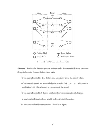
• a functional node sends to variable nodes intrinsic information in the following sense
λ
(1)
int,i = log
P(Zi|X
(1)
i = 0)
P(Zi|X
(1)
i = 1)
= log
∑
x P(Zi|X
(1)
i = 0,X
(2)
i = x)exλ
(2)
ext,i
∑
x P(Zi|X(1)
i = 1,X(2)
i = x)exλ
(2)
ext,i
λ(2)
int,i = log
∑
x P(Zi|X
(2)
i = 0,X
(1)
i = x)exλ
(1)
ext,i
∑
x P(Zi|X
(2)
i = 1,X
(1)
i = x)exλ
(1)
ext,i
.
Design rate For i ∈ {1, 2}, the design rates of such a multi-user code are provided by [56,
Lemma 3]
Rd,i = 1 −
li
ri
−
li
ri
1
2L + 1
w + 1 − 2
w∑
j=0
( j
w
)ri
. (5.11)
Note that this rate goes to the usual rate 1 − li/ri as L goes to infinity for a fixed w.
Density Evolution equations for the BEC If x
(t)
i (resp. y
(t)
i ) corresponds to the prob-
ability that a variable-to-check (resp. a check-to-variable) message carries an erasure for user
i ∈ {1, 2}, the density evolutions (DE) equations are
y(1)
j = 1 − 1 −
1
w
w−1∑
k=0
y(1)
j−k
r1−1
(5.12)
x
(1)
j = ϵ +
1 − ϵ
2
1
w
w−1∑
k=0
y
(2)
j+k
l2
1
w
w−1∑
k=0
y
(1)
j+k
l1−1
(5.13)
y(2)
j = 1 − 1 −
1
w
w−1∑
k=0
y(2)
j−k
r2−1
(5.14)
x
(2)
j = ϵ +
1 − ϵ
2
1
w
w−1∑
k=0
y
(1)
j+k
l1
1
w
w−1∑
k=0
y
(2)
j+k
l2−1
, (5.15)
where
• x(i)
j denotes the average erasure probability sent from the variable node side to the check
node side for user i ∈ {1, 2}, for a node at position j ∈ −L, L ;
• y
(i)
j denotes the average erasure probability flowing from the check node side to the vari-
able node side for user i, for a node at position j ∈ −L, L + w − 1 .
108

5.3 Punctured LDPC Codes for the MAC
5.3.1 Code Construction
The code construction is an extension of the notion of code puncturing [54, 106] for the wiretap
channel to the two-way channel defined earlier. The puncturing scheme operates as follows.
1. Choose LDPC codes ( C1, C2) for the MAC [56] with parity-check matrices H1 and H2
of the same size.
2. Split the matrix H1 ∈ Mm−l,m(F2) as H1 = [A1 B1], with B1 ∈ GLm−l(F2). Similarly,
split the matrix H2 ∈ Mm−l,m(F2) as H2 = [A2 B2], with B2 ∈ GLm−l(F2).
3. Form the temporary codeword ˜Xm
1 = [m1,m′
1,s1] ∈ C1 with m1 ∈ Fk
2, m′
1 ∈ Fl−k
2 s1 =
[m1,m′
1]A⊺
1(B−1
1 )⊺
∈ Fm−l
2 . The second user does the same with ˜Xm
2 = [m2,m′
2,s2] ∈ C2
with m2 ∈ Fk
2, m′
2 ∈ Fl−k
2 s2 = [m2,m′
2]A⊺
2(B−1
2 )⊺
∈ Fm−l
2 .
4. Puncture this code by only keeping Xn
1 = [m′
1,s1] and Xn
2 = [m′
2,s2], with n = m − k.
Puncturing induces a nested linear code structure, which is an algebraic counterpart of the
binning suggested by information-theoretic proofs. The rate of the mothercode is denoted by
Rd ≜ l/m and the secret rate for user i ∈ {1, 2} by Ri ≜ k/n. If the fraction of punctured bit
is p,
p =
k
m
⇒ Ri ≜
k
n
=
k
m − k
=
p
1 − p
. (5.16)
The quantity
R′
i ≜
l − k
m − k
=
l − pm
m − pm
=
Rd − p
1 − p
(5.17)
represents the auxiliary message rate for user i ∈ {1, 2}.
Encoding Use the punctured LDPC codes for data transmission as follows. User 1 sets m1
to be the secret message, m′
1 the auxiliary message and s1 the check sum defined above, and
sends [m′
1,s1] over the channel. User 2 performs similar encoding with independent sequences
m2 and m′
2.
109

Decoding for the legitimate receivers If useri ∈ {1, 2} receivesri, its decoder performs
belief propagation with [?m−n,rn
i ] as the channel a priori since it has no access to the punctured
bits, to estimate ˜Xm
i .
Decoding for the virtual receiver To minimize the last term of (5.9), a virtual user
should be able to retrieve messages M′
1 and M′
2 provided (M1, M2,Zn). The decoder estimates
˜Xm
1 and ˜Xm
2 using its channel observation and knowing the punctured bits.
Puncturing increases the decoding capabilities of the virtual receiver, thus providing secrecy.
However, when the number of punctured symbol increases, the communication rate decreases.
5.3.2 Leakage Analysis
Consider the (l1, r1, l2, r2, L,w) ensemble for the MAC presented in the previous section.
From Charlie’s point of view, it consists in setting the a priori inputs of coupling nodes to the
actual value of m. The density evolution equations remain the same, but the initialization is
different. The a priori informations become
• Bob: [? . . .? , d′
i , e′
i ], therefore the density evolution initialization is
x(0)
=
|c|
n
+
n − |c|
n
ϵ.
• Charlie: [c, d′′
i , e′′
i ], therefore the density evolution initialization is
x(0)
=
n − |c|
n
ϵ.
Recall that since the virtual user must be able to recover (M′
1,M′
2) from (M1,M2,Yn), the
puncturing consists in providing the virtual user with the values of the messages at the punctured
position. If p denotes the puncturing rate, note that this is not equivalent to setting the erasure
probability topϵ in the density evolution equations derived in [56]. Indeed, whenever a symbol
is punctured, the virtual receiver obtains the values of x1 and x2 at this position, not x1 + x2;
therefore, not only the erasures are removed in positions of punctured bits, but the interferences
when the symbol pairs are (−1, 1) and (1, −1) are also resolved.
110

Variable-to-check equation A variable node returns an erasure if all of the following hap-
pens:
1. the variable node is not punctured, which occurs with probability 1 − p;
2. the l1 − 1 adjacent edges carry erroneous messages;
3. the received value is erased (with probability ϵ), or the received value corresponds to a
collision (with probability (1 − ϵ)/2) and the opposite variable node is unknown.
Therefore, the average probability of erasure is
x(1)
j = (1 − p) ϵ +
1 − ϵ
2
1
w
w−1∑
k=0
y(2)
j+k
l2
1
w
w−1∑
k=0
y(1)
j+k
l1−1
. (5.18)
Check-to-variable equation A check node sends an erasure to a variable node if at least
one of the r1 − 1 other adjacent edges is an erasure:
y
(1)
j = 1 − 1 −
1
w
w−1∑
k=0
x
(1)
j−k
r1−1
. (5.19)
Similar equations are obtained for user 2.
The following proposition allows to avoid the analysis of density evolution for every possible
pair of codewords.
Proposition 5.2 ([85]) The average behavior of the previous density evolution can be ob-
tained for Xn
1 corresponding to the all-zero codeword and Xn
2 corresponding to a type one-half
codeword (equal number of −1 and 1). In that case Xn = Xn
1 + Xn
2 = Xn
2 corresponds also to a
type one-half codeword.
Proof The proof can be found in [85] for the Z-channel and holds for the multiple-access
channel.
Assume that Xn
1 + Xn
2 is a type one-half codeword. Define the set
Hδ =
{
Xn
,
1
2
−
δ
√
n
⩽
1
n
wt(Xn
) ⩽
1
2
+
δ
√
n
}
.
111

The probability that a codeword does not belong to that set is small and because of the sym-
metries in the decoding scheme, the behavior of the decoder is the same for all type one-half
codewords. The analysis can be restricted to the codewords Xn
1 = 1 and Xn
2 = h, where h is of
type one-half.
Notice that a type one-half codeword Xn = Xn
1 + Xn
2 captures the behavior of the code
ensemble since, for the erasure multiple-access channel, it represents a sequence with half inter-
ferences and half known values, which is a typical interference pattern.
5.3.3 Reliability Analysis
Suppose the channel from user 1 to user 2 is a BEC(ϵ1) and the channel from user 2 to user
1 is a BEC(ϵ2). Puncturing the codewords is equivalent to increasing the erasure probability
respectively to p + ϵ1 and p + ϵ2. If the codes C1 and C2 respectively have threshold ϵ∗
1 and ϵ∗
2,
one can ensure reliable communications if
ϵ1 ⩽ ϵ∗
1 − p and ϵ2 ⩽ ϵ∗
2 − p. (5.20)
The code thresholds ϵ∗
1 and ϵ∗
2 can be found using the density evolution equations for the
(l, r, L,w) SC-LDPC code ensemble
∀j ∈ {1, 2}, yj = 1 − 1 −
1
w
w−1∑
k=0
yj−k
r−1
and xj = ϵ
1
w
w−1∑
k=0
yj+k
l−1
. (5.21)
For instance, ϵ∗(3, 6, 200, 3) = 0.4807, ϵ∗(4, 8, 200, 4) = 0.4893 and ϵ∗(5, 10, 200, 5) =
0.4908.
5.3.4 Numerical Results
The density evolution equations [85] with puncturing allow to determine the asymptotic be-
havior of the SC-LDPC code ensemble for different code parameters and puncturing rate p as
the blocklength goes to infinity. The erasure probability thresholds in Table 5.1 are computed
in various cases with the density evolution equations.
The secrecy performance of the scheme is measured by the leakage rate. Whenever the
threshold of the code ensemble is not exceeded, it is possible to decode auxiliary messages M′
1
112

Table 5.1 – Advantages of spatially coupled LDPC codes.
Code parameters (3,6,3,6)-MAC-LDPC (3,6,3,6,200,3)
p Rs ϵShannon Rp ϵ∗ δ Rp ϵ∗ δ
0 0 0.3333 0.5 0.1226 0.2107 0.4977 0.3322 0.0011
0.1 0.1111 0.4074 0.4444 0.2136 0.1938 0.4419 0.4052 0.0022
0.2 0.2500 0.5000 0.3750 0.3210 0.1790 0.3722 0.4958 0.0042
0.3 0.4286 0.6190 0.2857 0.4497 0.1693 0.2825 0.6109 0.0081
0.4 0.6667 0.7778 0.1667 0.6079 0.1699 0.1629 0.7621 0.0157
Code parameters (4,8,4,8,200,4) (5,10,5,10,200,5)
p Rs ϵShannon Rp ϵ∗ δ Rp ϵ∗ δ
0 0 0.3333 0.4965 0.3332 0.0001 0.4953 0.3333 0.0000
0.1 0.1111 0.4074 0.4406 0.4072 0.0002 0.4392 0.4074 0.0000
0.2 0.2500 0.5000 0.3706 0.4994 0.0006 0.3691 0.4999 0.0001
0.3 0.4286 0.6190 0.2807 0.6178 0.0012 0.2790 0.6188 0.0002
0.4 0.6667 0.7778 0.1609 0.7750 0.0028 0.1588 0.7772 0.0006
Note that the value Rp for p = 0 corresponds to the mothercode rate. The quantity δ corresponds to the gap
between ϵ∗ and ϵShannon.
and M′
2 provided M1, M2, and Zn, with a probability arbitrarily close to one. For a given code
C in the ensemble with threshold ϵ∗, if ϵ ⩾ ϵ∗, then L( C) ⩽ Csum(ϵ∗) − 2Rp, where Rp is the
auxiliary message rate given in (5.17).
In Figure 5.4, the leakage rate is plotted with respect to the secret and auxiliary message
rates. It shows that, the higher the number of punctured bits, the higher the secrecy rate is,
since the punctured part of the codewords carries secret messages. However, the leakage rate
increases because the gap between the erasure threshold and the Shannon limit increases with
the puncturing rate. Figure 5.4 also shows that coupled codes have better performances than
classical LDPC codes and that their performance improve as the degree increases. Leakage val-
ues smaller than 10−3 bits can be reached, meaning that, on average, less than one per thousand
bits is not secured. Finally, even if classical LDPC codes of degrees (4,8) and (5,10) do not work
for the multiple-access channel (see [56]), they can be used for secrecy. However, they exhibit
113

0 0.2 0.4 0.6 0.8 1
10
5
10
4
10
3
10
2
10
1
10
0
Communication rate (in b.p.c.u)
Leakage(inbits)
1 0.89 0.75 0.57 0.33 0
Auxiliary message rate (in b.p.c.u)
(3,6,200,1)
(3,6,200,2)
(3,6,200,3)
(4,8,200,1)
(4,8,200,2)
(4,8,200,3)
(4,8,200,4)
(5,10,200,5)
Secret message rate (b.p.c.u.)
Leakagerate(b.p.c.u.)
Figure 5.4 – Leakage v.s. communication rate for various codes and puncturing rates. Codes with w = 1
correspond to classical LDPC codes.
poor performance. For instance, the leakage rate is about 0.5 bits for a classical (4,8)-LDPC
code.
Finite length effects Density evolution shows that spatially coupled LDPC codes provide
good results for secrecy with low leakage rate. However, for actual codes, the effects of finite
length decrease the performance for two reasons:
• the difference between Csum and R′
1 + R′
2 may not be negligible since one must remain
below Csum(ϵ∗) to have P′
e small;
• if the probability of error is non-zero, the term H M′
1M′
2|M1M2Yn is not negligible and
the upper bound on the leakage worsens.
Consequently, the predicted performances of actual codes can be far from asymptotic results.
For instance, spatially coupled codes with L = 25, M = 216, l = 3, r = 6, w = 3, and
114

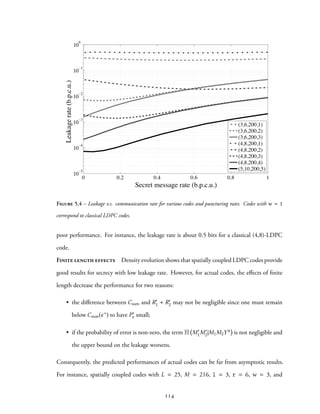
n = 11,016 bits provide leakage rate in the order of one half, which is far from the expected
asymptotic performances for such codes. Even if these codes appears to be better than a classical
LDPC code, they are not sufficient to provide low leakage rate.
These poor performances are likely caused by the small size of the code and the looseness
of the upper bound. Studying longer codes and comparing their performances with other
constructions is a subject of future investigation.
Remark The previous scheme only provides weak secrecy and only guarantees a low leakage
rate. Constructions based on polar codes for the multiple-access channel [86], could provide
strong secrecy.
This chapter presents a constrcution based on spatially-coupled LDPC codes for coded cooper-
ative jamming over the two-way wiretap channel. The construction uses random puncturing to
design a nested code structure to create codebooks, whose codewords detrimentally interfere at
the eavesdropper’s terminal. Spatially-coupled LDPC codes show significant advantages over
classical LDPC codes in terms of leakage and secret rate. However, such a scheme presents
some limitations in a real setting.
• The design involves a random an uniform puncturing, which is not practical.
• The model relies on the assumption that the interferences are perfect because the channel
gains between Alice and Eve and between Bob and Eve are both unitary. Guaranteeing
perfect interference also requires a precise synchronization between the legitimate users,
which is challenging for a real communication system.
Uniform Puncturing In [54], the authors investigate the impact of replacing the random
puncturing by an optimized puncturing scheme obtained with Differential Evolution [91].
They show gains of up to 0.4 dB over random puncturing. However, it is unclear how these
conclusions extend to spatially-coupled LDPC codes over the two-way wiretap channel. If it
115

appears that a fixed puncturing pattern decreases the performance of the system, it is still possi-
ble to compensate the loss with a higher puncturing rate in practice. Increasing the puncturing
rate directly impacts the legitimate users since they would need to increase their transmit power
to compensate the rate loss.
Gain Imbalance The previous analysis relies on having equal gains to create perfect interfer-
ence. Such an assumption is rather unrealistic in a real wireless environment. An experimental
setting similar to the one presented in the previous section is a good way to assess the validity
of the model introduced in Section 5.1. The following experiment is conducted using WARP
programmable radios, which performs better than the USPRs presented in the previous chapter.
The experimental setting consists of the following.
1. Two WARP radios (Alice and Bob) separated by 1 m that communicate on the 11th
WLAN channel (2.462 GHz).
2. A third radio (Eve) that receives on the 11th WLAN channel and that can be moved to
different locations.
3. The first radio transmits a sinusoidal wave at 5 MHz, while the other transmits a sinu-
soidal wave at 5.2 MHz.
4. The third radio uses the waves to compute the received gains GAE and GBE.
5. All the terminals are connected to the same computer and synchronized. The radios all
use the same type of isotropic antenna and the transmit gains for Alice and Bob are the
same.
Figure 5.5 shows how the gains GAE and GBE are actually imbalanced at the third radio
terminal. The left side of the map represents the theoretical behavior one could expect from
the simplified Friis equation [34],
Pr
Pt
= GtGr
(
λ
4πd
)2
. (5.22)
116

+1m +2m-1m 0m-2m
+1m
+2m
-1m
0m
-2m
Alice
Bob
Theoretical Experimental
20dB
-20dB
-10dB
0dB
10dB
Figure 5.5 – Gain imbalance between GAE and GBE.
This equation represents the ratio of the received power Pr to the transmitted power Pt for
isotropic receiving and transmitting antennas with respective gains Gr and Gt separated by a
distance d; additionally, λ corresponds the wavelength of the carrier frequency. If both transmit
antennas have the same gain, the gain ratio GAE to GBE in decibel is simply
GAE
GBE dB
= 20 log10
dBE
dAE
, (5.23)
wheredAE anddBE respectively represent the distances between Alice and Eve and between Alice
and Bob. The left-hand side of the map in Figure 5.5 shows this theoretical gain imbalance,
while the right-hand side corresponds the actual gain imbalance measured with the WARPS.
Figure 5.5 shows that, in theory, gains should be balanced if Eve is far enough from Alice
and Bob; however, experimental measurements show that this is not the case in a real wireless
setting. There are several reasons that can explain this difference.
117

• Equation (5.22) is a very simple approximation of the path loss that does not take into
account some properties of the antennas, such as their imperfect isotropy, their reflection
coefficient of the antennas, and their polarization vectors.
• The environment is not free space, and the presence of reflecting and absorbing objects
also affects the propagation of the wireless signal.
Managing this gain imbalance at the eavesdropper’s terminal is challenging, but one can
consider the following workarounds.
• The simple solution would consist in compensating the gain imbalance by adapting the
transmit power of Alice and Bob’s terminal. However, this solution requires a good
knowledge of Eve’s statistics.
• The best way to theoretically guarantee the performances of the coded cooperative jam-
ming code is to refine the model presented in Section 5.1 to account for the gain im-
balance. This solution is rather complicated since there is no simple degraded channel
model in that case.
• Finally, one could design codes based on the simple theoretical model presented in Sec-
tion 5.1 and verify how they perform in a real setting.
Terminal Synchronization The synchronization between Alice and Bob is another criti-
cal element to guarantee perfect interference at eve’s terminal. If the codewords are not fully
synchronized, the eavesdropper can gain additional information regarding the transmitted code-
words. The radios should transmit codewords at the same time with each bit perfectly aligned,
but it is also important to have synchronized local oscillators so that the signals are modulated
at exactly the same frequency. Software-defined radios can achieve both goals, either by using
an external clock or by using a GPS disciplined oscillator (GPSDO).
118

CHAPTER 6
CONCLUSION
6.1 Contributions
This dissertation has developed a comprehensive study of the coding mechanisms for multi-
user physical layer security, with a particular emphasis on understanding how to best exploit
interference and feedback for secrecy. The originality of the study lies in the combination of in-
formation theory, coding theory, and experiments conducted with software-defined radio. The
results obtain have confirmed the promising possibilities of multi-user physical layer security
but have also highlighted some of the practical challenges faced when deploying physical-layer
security systems in a real wireless setting.
Chapter 2 has introduced the basic information-theoretic primitives and technical tools
required to develop physical layer security schemes. In particular, this chapter has emphasized
the crucial roles of channel resolvability and channel intrinsic randomness as primitives for
the design of strongly secure schemes. One original result developed in this chapter is a joint
exponent of channel resolvability and channel intrinsic randomness, which illustrates how to
use some of the more intricate proof techniques required in subsequent chapters.
From the primitives presented in Chapter 2, Chapter 3 has developed an information-
theoretic analysis of the coding mechanisms for the two-way wiretap channel. In particular,
the analysis combines resolvability results for the multiple-access channel with secret-key gen-
eration and secret-key exchange. The resulting communication scheme has improved the state
of the art by not only providing strong secrecy but also increasing the set of known achievable
rates. The performance of this coding scheme has been illustrated for the Gaussian two-way
wiretap channel, which is a model of practical interest.
Motivated by the crucial role of secret-key generation for the coding scheme in the coding
scheme of Chapter 3, Chapter 4 has examined the practical limitations of a secret-key genera-
tion system in a real wireless setting. In particular, the study has focused on commonly made
119

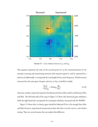
assumptions regarding the reciprocity and diversity of the wireless channel. The rate penalty
incurred by the use of a final number of samples as well as imperfect diversity and reciprocity
have been precisely quantified using experimental channel gain measurements acquired with
software-defined radios. While the results do not compromise the validity of the approach,
they do suggest that many previously reported results may be overly optimistic.
Finally, Chapter 5 has proposed a code construction for the Gaussian two-way wiretap
channel based on spatially-coupled LDPC codes. The resulting coding scheme exhibits low
leakage rate but relies on perfect interferences at the eavesdropper’s terminal, thus requiring
good synchronization between the legitimate parties. This chapter has also investigated some
of the limitations of the model used to design codes by comparing it again experimental mea-
surements.
6.2 Perspectives
The work presented in this dissertation could be extended in several directions.
Strongly secure practical coded cooperative jamming codes The codes developed
in Chapter 5 only offer weak secrecy. Polar codes could be used to provide strong secrecy [22],
but the construction of low-complexity codes with good performance at reasonable block length
might prove challenging.
Implementation of practical coded cooperative jamming schemes As discussed in
Chapter 5, it may be challenging to design a practical coded cooperative jamming scheme since
codeword interference is not a simple signal addition. As in Chapter 4, it would be valuable to
implement such a system on software-defined radios to assess its performances in a real wireless
environment. Since coded cooperative jamming requires an almost perfect synchronization of
the terminals, it is important to assess the impact of imperfect synchronization on the overall
secrecy rate. One could also expect that the position of the eavesdropper affects its abilities
to gather information about the legitimate communications, although recent works [44, 45]
suggest that this could be circumvented.
120

Hybrid solutions Chapter 4 describes how to generate a secret key between different termi-
nals, but it does not investigate how the secret-key could be later used to provide secrecy. One
could imagine a situation in which the secret-key serves in classical cryptographic primitives.
For instance, one could used secret-key generation to refresh the WPA key of a Wi-Fi network
periodically. This hybrid solution using both physical-layer security and cryptography would
offer an additional layer of protection at no cost. The difficulty lies in the analysis of the overall
solution since physical-layer security and cryptography do not rely on the same tools. Recent
results [71] offer promising research directions.
121

CHAPTER 7
APPENDIX
7.1 Coding with Polar Codes
It is difficult to provide a simple joint coding scheme based on polar codes for the problem
considered in Section 2.3. However, this appendix briefly illustrates how polar codes achieve
the maximal achievable rates for some sources and channels with a separate approach. What
follows assumes that n ≜ 2m for some m ∈ N.
For channel intrinsic randomness, consider the situation where Zn is i.i.d. and B(ζ ), and
Xn is such that Xn = Zn ⊕W n withWn i.i.d. B(ω) and independent of Zn. Polar codes (see [7]
for notation) are used to encode Xn, the output of the encoder is denoted Un = XnG⊗m, where
G⊗m is the Arıkan transform. For δn ≜ 2−nβ
with β ∈ (0; 1/2), define the bit sets
Gcir
n ≜ i ∈ 1,n , H Ui|Ui−1
Zn
⩾ 1 − δn , (7.1)
Bcir
n ≜ ∁ 1,n Gcir
n . (7.2)
One can then show [1, 22] that
lim
n→∞
log | Gcir
n |
n
= H(X|Z) and lim
n→∞
D
(
pU [ Gcir
n ]Zn qUnqZn
)
= 0, (7.3)
where pU [ Gcir
n ] is the distribution of the bits of Un in position Gcir
n and qUn ≜ U 1, 2nR .
For channel resolvability, if ˜Yn is i.i.d. according to B(1/2) and if the channel W2 is sym-
metric, the corresponding channel output ˜Kn is simulated as follows. Sequence Yn is created
from an n bit sequence Vn as Yn = VnG⊗n. The bits of Vn belong to either one of the sets
Gres
n ≜
{
i ∈ 1,n ,C
(
W
(i)
n
)
⩾ δn
}
and Bres
n ≜ ∁ 1,n Gres
n , (7.4)
where C(W
(i)
n ) is the capacity of the i -th bit-channel for bit Vi. If uniform bits are transmitted
in positions Gres
n , references [15, 64] prove that these codes are channel resolvability codes of
rate I ˜Y; ˜K , i.e.
lim
n→∞
log | Gres
n |
n
= I ˜Y; ˜K and lim
n→∞
D(pKn ∥qKn ) = 0. (7.5)
122

Consequently, one can combine channel intrinsic randomness and channel resolvability by
transmitting the nearly uniform bits of Un obtained in positions Gcir
n on the position Gres
n of
Vn, which is possible if H(X|Z) > I( ˜Y; ˜K).
The solution in [64] guarantees both weak secrecy and reliability, but does not ensure reli-
ability under a strong secrecy criterion. A solution to this problem consists in designing multi-
block polar coding schemes with a secret-key exchange mechanism used to encrypt part of
the non-secure bits [22, 87]. Such a construction achieves the secrecy capacity of symmetric
degraded wiretap channels while also ensuring reliability.
7.2 Universal Software Radio Peripherals (USRPs)
USRPs (Universal Software Radio Peripheral) [31] are software-defined radios that can be used
to communicate in various frequency ranges (DC-5GHz). USRPs are commonly used with
the GNURadio [36] software suite that offers a wide range of possibilities for experimental
communication systems.
Figure 7.1 – USRP1 with two daughterboards plugged in.
At a high level, the architecture of a USRP presented in Figures 7.1 and 7.2 consists of a
motherboard and between one and four daughterboards. The motherboard handles the process-
ing of baseband signals while the daughterboards are designed to achieve frequency translation
of the baseband signals.
123

Table 7.1 – Comparisons of the different USPR models.
Features USRP1 N200 N210 E100 E110 E310 B200 B210 X300 X310
FPGA Altera
Cyclone
Spartan
3A1800
Spartan
3A3400
OMAP3
720 MHz
OMAP3
720 MHz
Zynq
7020
Spartan
675
Spartan
6150
Kintex7
325T
Kintex7
410T
Min freq. DC DC DC DC DC 70 MHz 70 MHz 70 MHz DC DC
Max freq. 6 GHz 6 GHz 6 GHz 6 GHz 6 GHz 6 GHz 6 GHz 6 GHz 6 GHz 6 GHz
Bandwidth 16 MHz 50 MHz 50 MHz 8 MHz 8 MHz 56 MHz 56 MHz 56 MHz 120 MHz 120 MHz
Connection USB 2.0 GbE GbE GbE GbE GbE/USB USB 3.0 USB 3.0 GbE GbE
MIMO ✓opt ✓opt ✓opt × × ✓ × ✓ ✓ ✓
DBoards ✓ ✓ ✓ ✓ ✓ × × × ✓ ✓
Standalone × × × ✓ ✓ ✓ × × × ×
GPS Sync ✓opt ✓opt ✓opt ✓opt ✓opt ✓ ✓opt ✓opt ✓opt ✓opt
Price $707 $1,515 $1,717 $1,310 $1,515 $2,700 $675 $1,100 $3,900 $4,800
There is a wide family daughterboards, covering different frequency bands from DC to
5 GHz. While the experiments described in Chapter 4 are performed with the first version of
the USRP, several new versions have came out with improved characteristics. The current offer
by Ettus is summarized in Table 7.1.
According to the frequency range used, different antennas may be used. Most experiments
were performed in the 2.5 GHz and 5 GHz bands. The Wi-Fi-compliant antennas are perfectly
adapted to transmit these signals. Although the center frequencies are 2.5 GHz and 5 GHz, the
emission bandwidth is limited by the transfer speeds of the USB port to 8 MHz. This limitation
makes USRPs incompatible with the IEEE802.11 protocol.
Figure 7.3 provides a representation of the internal operation of a USRP:
FPGA The FPGA (Field-Programmable Gate Array) performs many preprocessing operations
to allow data to be transmitted through the USB port. The FPGA and the USB controller to
which it is connected, are fully programmable via USB2.0. The FPGA is in charge of the
124

RXB
TXB
+3.3V
ANALOG
DEVICE
MxFE
AD9862
USB
Controler
ALTERA
Cyclone
EP1C12Q240C8
L BCC9S0513A
TXA
RXA
GNURadio Rev 3
1-3-2005
ANALOG
DEVICE
MxFE
AD9862
XCVR2450 REV
2.4GHz and 5 GHz Transceiver
Copyright 2007 Ettus Research LLC
+ +
+
+ +
+
+
I0I0
MA
XIM
+
Daughterboard
Large Band
Communication
Processor
USB Port
6VDC Power
FPGA
USB Controller
SMA Connector
Daughterboard
Connector
Figure 7.2 – Overview of a software-defined radio (USRP1).
distribution of signals between different daughterboards. It also allows various operations such
as interpolation and decimation.
Analog/Digital converters The motherboard has four A/D converters of 12 bits. The
sampling rate of the converter is 64 million samples per second. Although ADCs have a cutoff
frequency of 150 MHz, if the bandwidth is greater than 32 MHz aliasing may occur. It is
possible to use other sampling frequencies whenever they are in multiples of 128 MHz.
The board also contains four digital/analog converters of 14 bits. The sampling rate is
128 MHz. While the Shannon frequency is 64 MHz, it is best to stay below 50 MHz to make
filtering easier. This offers a total of four inputs and four outputs with real numbers or two
inputs and two outputs with complex numbers.
Daughterboards Daughterboards are pluggable circuits that, depending on the model,
have different features. The motherboard can accommodate two Rx boards and two Tx boards
or two dual mode transmitter boards. These boards are in charge of frequency translation. Each
board has two SMA connectors for connecting the card to the antennas. Several daughterboards
are available:
125

F
P
G
A TX Board
B
DAC
DAC
DAC
DAC
ADC
ADC
ADC
ADC
RX Board
B
TX Board
A
RX Board
A
USB
Figure 7.3 – General diagram of a software-defined radio.
• Basic RX / Basic TX: these boards do not perform any operation apart from connecting
the converters outputs to SMA connectors.
• LFRX / LFTX: it is quite similar to the two previous boards, except that they include
differential amplifiers to work with continuous signals.
• TVRX: Equipped with a MicroTuner, it can receive UHF and VHF signals and is there-
fore useful for receiving FM signals or TV.
• DBSRX: it can translate the baseband signals to frequencies between around 800 MHz
and 2.4GHz. It also contains a channel filter adjustable between 1 MHz and 60 MHz.
• XCVR2450: it can work in the frequency range of IEEE 802.11n. It works in both
transmission and reception. This is the board that is used for the experiments described
in Chapter 4.
The ease of use software-defined radios largely stems from the fact that most of the processing is
performed on baseband signals. The general idea is to observe that a bounded spectrum signal
can be seen as a signal in baseband (centered around zero frequency) modulated by a signal
of desired frequency. The modulation frequency corresponds to a translation of the signal
spectrum.
126

Signal en bande de base Signal modulé
modulation
f f
f0
Figure 7.4 – Modulation.
Signal emission Several steps are necessary to emit a signal and are summarized in Figure 7.5
below.
AD9862
Interpolator
Fine
Modulation
Coarse
Modulation
s(t)
FPGA
4th Order
Interpolator
Gain
↑R↑R DACG
exp(2 0n) exp(2 1n)
Figure 7.5 – Signal modulation and transmission.
The main steps are:
• Interpolation: to avoid clogging the USB port, the interpolator transmits only some of
the points needed to represent signals. The interpolation is then necessary to achieve the
number of samples the DAC needs. However, it is important to note that the interpola-
tion rate affects the bandwidth of the transmitted signal.
• Coarse modulation: a first modulation allows coarsely approaching the center frequency
of the desired modulation.
• Fine modulation: a second modulation allows precisely adjusting the center frequency
of translation.
127

• Gain: A variable gain allows adapting the amplitude of signals to be transmitted at the
level necessary to emit the wave with the antennas.
• Digital/Analog conversion: Finally, the digital signal is converted into an analog signal
to be transmitted by the antennas in the form of an electromagnetic wave.
FPGAAD9862
Demodulation
4th Order
Decimator
Gain Half-band
Decimator
G ADC ↓R ↓R
exp(2 1n)
Figure 7.6 – Signal reception and demodulation.
Signal Reception The reception is performed with a mechanism similar to that of the emis-
sion. Again, it is important to be attentive to the decimation rate used. The higher this rate, the
narrower the bandwidth of the received signal is. The demodulation is done only once. If the
modulation and demodulation frequencies are slightly different (which is the case with asyn-
chronous transmission), a modulation frequency (equal to the difference between the deviation
of the frequency modulation and demodulation) will appear. It is necessary to find mechanisms
to overcome this issue.
7.3 Proofs of Lemmas
7.3.1 Proof of Lemma 3.2
Define: M1 ≜ 2R1 , M2 ≜ 2R2 , M′
1 ≜ 2R′
1 and M′
2 ≜ 2R′
2 , and let C be the random
variable representing a randomly generated code. Let ϵ > 0.
128

Without loss of generality, the analysis can be restricted to the transmission of a single message
since
E(Pe(C)) = E
∑
µ1∈M1×M′
1
∑
µ2∈M2×M′
2
Pe(C|µ1, µ2 sent)P(µ1, µ2 sent)
=
∑
µ1∈M1×M′
1
∑
µ2∈M2×M′
2
P(µ1, µ2 sent) EC(Pe(C|µ1, µ2 sent))
EC (Pe(C|1,1 sent))
(a)
= E(Pe(C|1, 1 sent))
(b)
⩽ E(P(µ1 ˆµ1|1, 1 sent,C)) + E(P(µ2 ˆµ2|1, 1 sent,C)). (7.6)
Equality (a) follows from the symmetry of the random code construction, while inequality (b)
comes from the union bound.
Each term can be expressed using the following events:
• E(i, j) =
{
Xn
1 ,Cn
2(i, j),Yn
1 ∈ An
1,ϵ
}
• F(i, j) =
{
Xn
2 ,Cn
1(i, j),Yn
2 ∈ An
2,ϵ
}
The probability of error is therefore
E(P(µ2 ˆµ2|1, 1 sent,C)) = P
(
Ec
(1, 1) ∪
∪
(i,j) 1
E(i, j)
)
⩽ P(Ec
(1, 1))
⩽δ(ϵ)
+
∑
(i,j) 1
P(E(i, j)) (7.7)
∑
(i,j) 1
P(E(i, j)) ⩽ δ(ϵ) +
∑
(i,j) 1
∑
(xn
1 ,cn
2 ,yn
1 )∈An
1,ϵ
pXn
1 Yn
1
(xn
1,cn
1)pCn
2
(cn
2)
⩽ δ(ϵ) + M2M′
2
⩽ 2n(R2+R′
2+δ(n))
2n(H(X1C2Y1)+ϵ)
2−n(H(C2)−ϵ)
2−n(H(X1Y1)−ϵ)
= δ(ϵ) + 2n(R2+R′
2−I(C2;Y1|X1)+δ(n)+3ϵ)
. (7.8)
Remark The second inequality follows from the union bound and the penultimate from the
AEP.
129

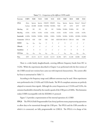
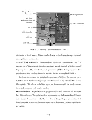
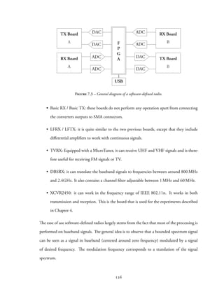
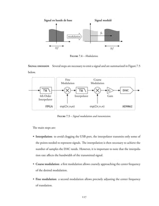
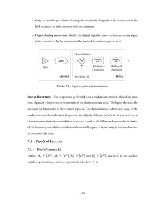
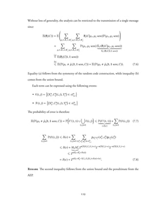
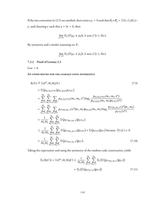
An upper bound for the divergence:
D(pZn|1,1, C∥pZn ) =
∑
zn ∈Zn
pZn|1,1, C(zn
) log2
pZn|1,1, C(zn)
pZn (zn)
=
∑
zn ∈Zn
pZn|1,1, C(zn
) log2
pZn|1,1, C(zn)
pZn (zn)
1
{
pZn|1,1, C(zn)
pZn (zn)
⩽ ϵ
}
+
∑
zn ∈Zn
pZn|1,1, C(zn
) log2
pZn|1,1, C(zn)
pZn (zn)
1
{
pZn|1,1, C(zn)
pZn (zn)
> ϵ
}
⩽ ϵ +
∑
zn ∈Zn
pZn|1,1, C(zn
) log2
pZn|1,1, C(zn)
pZn (zn)
1
{
pZn|1,1, C(zn)
pZn (zn)
> ϵ
}
. (7.12)
By the law of total probability:
pZn (zn
) =
∑
cn
1 ∈ Cn
1
∑
cn
2 ∈ Cn
2
pZn|Cn
1 Cn
2
zn
|cn
1,cn
2 pCn
1
cn
1 pCn
2
cn
2
⩾
∑
cn
1 ∈B1(1)
∑
cn
2 ∈B2(1)
pZn|Cn
1 Cn
2
zn
|cn
1,cn
2 pCn
1
cn
1 pCn
2
cn
2
⩾ M′
1M′
2pn
min1
pn
min2
pn
min
pZn|1,1, C(zn
) ,
where Bi(m), for i ∈ {1, 2}, represents the set of codewords associated with message m for user
i. To obtain the last inequality, the p.d.f. of C1 and C2 must have compact support, which
can always be obtained by cropping (to get a compact support) and scaling (to keep an unit
area) the p.d.f. If ˇC1 and ˇC2 are derived from C1 and C2 with discrete or Gaussian p.d.f., it
is possible to get V
(
pC1,p ˇC1
)
and V
(
pC2,p ˇC2
)
as small as desired. Since I(X;Y) viewed as a
function of pX , with pY|X fixed, is continuous, the mutual informations involved in (3.7) are
hardly modified by using ˇC1 and ˇC2 instead of C1 and C2.
By taking the expectation of (7.12) and with [90],
EC(L(C)) = I(Zn
; M1M2|C) ⩽ ϵ + n log2
(
1
pmin
)
Jϵ, (7.13)
131

where Jϵ is defined as:
Jϵ ≜
∑
c
(2)
1 ∈ Cn
1
· · ·
∑
c
(M′
1)
1 ∈ Cn
1
∑
c
(2)
2 ∈ Cn
2
· · ·
∑
c
(M′
2)
2 ∈ Cn
2
pCn
1
(
c
(2)
1
)
· · ·pCn
1
(
c
(M′
1)
1
)
pCn
2
(
c
(2)
2
)
· · ·pCn
2
(
c
(M′
2)
2
)
×
∑
c
(1)
1 ∈ Cn
1
∑
c
(1)
2 ∈ Cn
2
∑
zn ∈Zn
pCn
1 Cn
2 Zn
(
c(1)
1 ,c(1)
2 ,zn
)
1
{
1
M′
1M′
2
exp2
(
iCn
1 Cn
2 ;Zn
(
c
(1)
1 ,c
(1)
2 ;zn
))
+
1
M′
1M′
2
∑
(i,j) (1,1)
exp2
(
iCn
1 Cn
2 ;Zn
(
c
(i)
1 ,c
(j)
2 ;zn
))
> 1 + 4ϵ
}
.
An upper bound for Jϵ: Recall the following assumption from (3.7):



R′
1 + R′
2 > I(C1C2;Z)
R′
1 > I(C1;Z)
R′
2 > I(C2;Z)
The quantity Jϵ can be upper bounded as (see [90]):
Jϵ ⩽ J(1)
+ J(2)
+ J(3)
+ J(4)
, (7.14)
where J(1), J(2), J(3), and J(4) are defined as:
J(1)
= P
( 1
M′
1M′
2
exp2
(
iCn
1 Cn
2 ;Zn
(
C
(1)
1 C
(1)
2 ;Zn
))
> ϵ
)
J(2)
= P
( 1
M′
1M′
2
n∑
i=1
n∑
j=1
exp2
(
iCn
1 Cn
2 ;Zn
(
C(i)
1 C(j)
2 ;Zn
))
> 1 + ϵ
)
J(3)
= P
( 1
M′
1M′
2
n∑
i=1
exp2
(
iCn
1 Cn
2 ;Zn
(
C(i)
1 C(1)
2 ;Zn
))
> ϵ
)
J(4)
= P
( 1
M′
1M′
2
n∑
j=1
exp2
(
iCn
1 Cn
2 ;Zn
(
C(1)
1 C(j)
2 ;Zn
))
> ϵ
)
.
Now, each term are studied individually.
• First, J(1) can be upper bounded as follows:
J(1)
⩽ P(exp2(I Cn
1Cn
2;Zn
) > exp2(−nϵ + nR′
1 + nR′
2))
= P
(1
n
I Cn
1Cn
2;Zn
> −ϵ + R′
1 + R′
2
)
= P
1
n
n∑
i=1
I C1,iC2,i;Zi > R′
1 + R′
2 − ϵ
132

since R′
1 + R′
2 > I(C1C2;Z), there exists γ > 0 such that R′
1 + R′
2 > I(C1C2;Z) + γ. By
taking ϵ < γ to guarantee R′
1 + R′
2 − ϵ > I(C1C2;Z) + γ − ϵ
>0
and to apply the Chernoff
bound, then
∃αγ−ϵ > 0, J(1)
⩽ e−αγ −ϵn
.
• With a similar reasoning, the terms J(2), J(3), and J(4) can also be upper bounded by
quantities going exponentially to zero under the given conditions.
Conclusion: Jϵ goes exponentially to zero as n goes to infinity. Therefore,
lim
n→∞
E(L(C)) ⩽ δ(ϵ).
Define the joint distribution qXn
1 Xn
2 Zn as
∀(xn
1,xn
2,zn
) ∈ Xn
1 × Xn
2 × Zn
, qXn
1 Xn
2 Zn (xn
1,xn
2,zn
) = pZn|Xn
1 Xn
2
(zn
|xn
1xn
2 )pXn
1
(xn
1 )pXn
2
(xn
2 ).
First, the variational distance between distributionspM1M2Zn andpM1M2pZn can be upper bounded
as
V(pM1M2Zn ,pM1M2pZn ) = EM1M2 (V(pZn|M1M2
,pZn ))
⩽ EM1M2 ((V(pZn|M1M2
,qZn ) + (V(qZn ,pZn ))
⩽ 2EM1M2 ((V(pZn|M1M2
,qZn )), (7.15)
By averaging over every code and by symmetry of the random code construction,
ECn (V(pM1M2Zn ,pM1M2pZn )) ⩽ 2ECn (V(pZn|M1=1,M2=1,qZn )),
where
pZn|M1=1,M2=1(zn
) =
M′
1∑
m′
1=1
M′
2∑
m′
2=1
WZn|Xn
1 Xn
2
(zn
|xn
1 (1,m′
1),xn
2 (1,m′
2))pM′
1
(m′
1)pM′
2
(m′
2).
133

For any zn ∈ Zn,
ECn pZn|M1=1,M2=1 = ECn
M′
1∑
m′
1=1
M′
2∑
m′
2=1
WZn|Xn
1 Xn
2
(zn
|xn
1 (1,m′
1),xn
2 (1,m′
2))pM′
1
(m′
1)pM′
2
(m′
2)
=
M′
1∑
m′
1=1
M′
2∑
m′
2=1
ECn
(
WZn|Xn
1 Xn
2
(zn
|xn
1 (1,m′
1),xn
2 (1,m′
2))
)
pM′
1
(m′
1)pM′
2
(m′
2)
= qZn (zn
). (7.16)
Now define
p(1)
(zn
) ≜
M′
1∑
m′
1=1
M′
2∑
m′
2=1
WZn|Xn
1 Xn
2
(zn
|xn
1 (1,m′
1),xn
2 (1,m′
2))pM′
1
(m′
1)pM′
2
(m′
2)
×1{(xn
1 (1,m′
1),xn
2 (1,m′
2),zn
) ∈ Tn
ϵ (X1X2Z)}
p(2)
(zn
) ≜
M′
1∑
m′
1=1
M′
2∑
m′
2=1
WZn|Xn
1 Xn
2
(zn
|xn
1 (1,m′
1),xn
2 (1,m′
2))pM′
1
(m′
1)pM′
2
(m′
2)
×1{(xn
1 (1,m′
1),xn
2 (1,m′
2),zn
) Tn
ϵ (X1X2Z)},
which are used to upper bound V(pZn|M1=1,M2=1,qZn ) as
V(pZn|M1=1,M2=1,qZn ) ⩽
∑
zn Tn
ϵ (Z)
|pZn|M1=1,M2=1(zn
) − qZn (zn
)|
+
∑
zn ∈Tn
ϵ (Z)
p(1)
(zn
) − E(p(1)
(zn
)) +
∑
zn ∈Tn
ϵ (Z)
p(2)
(zn
) − E(p(2)
(zn
))
The first and last terms involving non-typical and non-jointly typical sequences vanish as n goes
to infinity. By using Jensen’s inequality, the concavity of x →
√
x guarantees
E p(1)
(zn
) − E(p(1)
(zn
)) ⩽
√
Var(p(1)(zn))
134

The variance of Var(p(1)(zn)) is
Var(p(1)
(zn
)) ⩽
M′
1∑
m′
1=1
M′
2∑
m′
2=1
pM′
1
(m′
1)2
pM′
2
(m′
2)2
E W 2
Zn|Xn
1 Xn
2
(zn
|Xn
1 (1, 1),Xn
2 (1, 1))
×1{(Xn
1 (1, 1),Xn
2 (1, 1),zn
) ∈ Tn
ϵ (X1X2Z)}
+
M′
1∑
m′
1=1
pM′
1
(m′
1)2
E WZn|Xn
1 Xn
2
(zn
|Xn
1 (1, 1),Xn
2 (1, 1))
×WZn|Xn
1 Xn
2
(zn
|Xn
1 (1, 1),Xn
2 (1, 2))1{(Xn
1 (1, 1),Xn
2 (1, 2),zn
) ∈ Tn
ϵ (X1X2Z)}
+
M′
2∑
m′
2=1
pM′
2
(m′
2)2
E WZn|Xn
1 Xn
2
(zn
|xn
1 (1, 1),xn
2 (1, 1))
×WZn|Xn
1 Xn
2
(zn
|Xn
1 (1, 2),Xn
2 (1, 1))1{(Xn
1 (1, 2),Xn
2 (1, 1),zn
) ∈ Tn
ϵ (X1X2Z)}
Using the AEP on the first term yields
E W 2
Zn|Xn
1 Xn
2
(zn
|Xn
1 (1, 1),Xn
2 (1, 1))1{(Xn
1 (1, 1),Xn
2 (1, 1),zn
) ∈ Tn
ϵ (X1X2Z)}
⩽ exp2(−n(H(Z|X1X2) + H(Z) − δϵ)). (7.17)
Similarly, the second term is upper bounded by
E WZn|Xn
1 Xn
2
(zn
|Xn
1 (1, 1),Xn
2 (1, 1))WZn|Xn
1 Xn
2
(zn
|Xn
1 (1, 1),Xn
2 (1, 2))
× 1{(Xn
1 (1, 1),Xn
2 (1, 2),zn
) ∈ Tn
ϵ (X1X2Z)}
⩽ exp2(−n(H(Z|X1) + H(Z) − δϵ)), (7.18)
and the third term by
E WZn|Xn
1 Xn
2
(zn
|Xn
1 (1, 1),Xn
2 (1, 1))WZn|Xn
1 Xn
2
(zn
|Xn
1 (1, 2),Xn
2 (1, 1))
× 1{(Xn
1 (1, 2),Xn
2 (1, 1),zn
) ∈ Tn
ϵ (X1X2Z)}
⩽ exp2(−n(H(Z|X2) + H(Z) − δϵ)). (7.19)
135

Combining the previous upper bounds,
Var(p(1)
(zn
)) ⩽
M′
1∑
m′
1=1
M′
2∑
m′
2=1
pM′
1
(m′
1)2
pM′
2
(m′
2)2
exp2(−n(H(Z|X1X2) + H(Z) − δϵ))
+
M′
1∑
m′
1=1
pM′
1
(m′
1)2
exp2(−n(H(Z|X1) + H(Z) − δϵ))
+
M′
2∑
m′
2=1
pM′
2
(m′
2)2
exp2(−n(H(Z|X2) + H(Z) − δϵ))
= exp2(−H2(M′
1M′
2) − n(H(Z|X1X2) + H(Z) − δϵ))
+ exp2(−H2(M′
1) − n(H(Z|X1) + H(Z) − δϵ))
+ exp2(−H2(M′
2) − n(H(Z|X2) + H(Z) − δϵ)),
where H2 is the second order Rényi entropy. Finally,
∑
zn ∈Tn
ϵ (Z)
p(1)
(zn
) − E
(
p(1)
(zn
)
)
⩽ exp2(H(Z)) exp2
(
−
n
2
(1
n
H2(M′
1M′
2) + H(Z|X1X2) + H(Z) − δϵ
))
+ exp2(H(Z)) exp2
(
−
n
2
(1
n
H2(M′
1) + H(Z|X1) + H(Z) − δϵ
))
+ exp2(H(Z)) exp2
(
−
n
2
(1
n
H2(M′
2) + H(Z|X2) + H(Z) − δϵ
))
,
= exp2
(
−
n
2
(
H2(M′
1M′
2)
n
+ I(X1X2;Z) − δϵ
))
+ exp2
(
−
n
2
(
H2(M′
1)
n
+ I(X1;Z) − δϵ
))
+ exp2
(
−
n
2
(
H2(M′
2)
n
+ I(X2;Z) − δϵ
))
, (7.20)
Therefore, if
lim
n→∞
1
n
H2(M′
1, M′
2) > I(X1X2;Z), lim
n→∞
1
n
H2(M′
1) > I(X1;Z), and lim
n→∞
1
n
H2(M′
2) > I(X2;Z),
(7.21)
the sum vanishes as n goes to infinity.
136

Let i ∈ 1, B − 1 . We have
Li+1 − Li = I
(
M1,1:BM′
1,2:BM2,1:B;Zn
1:i+1
)
− I
(
M1,1:BM′
1,2:BM2,1:B;Zn
1:i
)
= I
(
M1,1:BM′
1,2:BM2,1:B;Zn
i+1 Zn
1:i
)
= I
(
M1,1:i+2:BM′
1,1:i+2:BM2,1:i+2:B;Zn
i+1 Zn
1:iM1,1:i+1M′
1,1:i+1M2,1:i+1
)
+I M1,1:i+1M′
1,2:i+1M2,1:i+1;Zn
i+1 Zn
1:i
(a)
⩽ I
(
M1,1:i+2:BM′
1,1:i+2:BM2,1:i+2:B;Zn
1:i+1M1,1:i+1M′
1,1:i+1M2,1:i+1
)
(7.22)
+I M1,1:i+1M′
1,2:i+1M2,1:i+1Zn
1:i;Zn
i+1
(b)
= I M1,1:i+1M′
1,2:i+1M2,1:i+1Zn
1:i;Zn
i+1 (7.23)
= I M1,i+1M′
1,i+1M2,i+1;Zn
i+1 + I M1,1:iM′
1,2:iM2,1:iZn
1:i;Zn
i+1 M1,i+1M′
1,i+1M2,i+1
(c)
⩽ δn(ϵ) + I M1,1:iM′
1,2:iM2,1:iZn
1:i;Zn
i+1 M1,i+1M′
1,i+1M2,i+1 (7.24)
⩽ δn(ϵ) + I M1,1:iM′
1,2:iM2,1:iZn
1:i;Zn
i+1M1,i+1M′
1,i+1M2,i+1
= δn(ϵ) + I M1,1:iM′
1,2:iM2,1:iZn
1:i; M1,i+1M′
1,i+1M2,i+1
+I M1,1:iM′
1,2:iM2,1:iZn
1:i;Zn
i+1 M1,i+1M′
1,i+1M2,i+1
= δn(ϵ) + I M1,1:iM′
1,2:iM2,1:iZn
1:i;Zn
i+1 M1,i+1M′
1,i+1M2,i+1
(d)
⩽ δn(ϵ) + I M1,1:iM′
1,2:iM2,1:iZn
1:i;Zn
i+1Pi+1Ki M1,i+1M′
1,i+1M2,i+1 (7.25)
= δn(ϵ) + I M1,1:iM′
1,2:iM2,1:iZn
1:i; Pi+1Ki M1,i+1M′
1,i+1M2,i+1
+I M1,1:iM′
1,2:iM2,1:iZn
1:i;Zn
i+1 Pi+1KiM1,i+1M′
1,i+1M2,i+1
(e)
⩽ δn(ϵ) + I Cn
1,1:iCn
2,1:iZn
1:i;KiPi+1 (7.26)
= δn(ϵ) + I Cn
1,iCn
2,iZn
i ;KiPi+1 + I Cn
1,1:i−1Cn
2,1:i−1Zn
1:i−1;KiPi+1 Cn
1,iCn
2,iZn
i
(f)
⩽ δn(ϵ), (7.27)
where (a) holds by the chain rule and positivity of mutual information, (b) holds by indepen-
dence of M1,1:i+2:BM′
1,2:i+2:BM2,1:i+2:B with all the random variables of the previous blocks, (c)
holds thanks to the result on secret-key generation, in (d) the random variables Pi+1 and Ki are
137

introduced, (e) holds because of the data processing inequality and because the conditioning on
Pi+1 and Ki breaks the dependencies between the random variables of block (i + 1) and the ran-
dom variables of the previous blocks, (f) holds because (Pi+1,Ki) and (Cn
1,1:i−1,Cn
2,1:i−1,Zn
1:i−1)
are independent and also because Pi+1 and Ki break the dependencies between consecutive
blocks.
To show that PU (Hϵ
∞ (S) − Hϵ
∞ (S|U = ¯u) > log |U| + r), first note that
Hϵ
∞ (S|U = ¯u) = max
qS ¯U ∈Bϵ (Su)
min
s∈S
log
pU (¯u)
qS ¯U (s, ¯u)
= − min
qS ¯U ∈Bϵ (Su)
max
s∈S
log (qS ¯U (s, ¯u)) + log (pU (¯u))
⩾ − min
qS ∈Bϵ (S)
max
s∈S
log (qS(s)) + log (pU (¯u))
= Hϵ
∞ (S) + log (pU (¯u)) (7.28)
where the inequality follows because for all (s,u) ∈ S × U, qS ¯U (s, ¯u) ⩽ pS(s). Hence,
PU (Hϵ
∞ (S) − Hϵ
∞ (S|U = ¯u) > log |U| + r) ⩽ P(logpU (U ) < − log |U| − r)
= P
(
pU (U ) <
2−r
|U|
)
=
∑
u∈U
pU (u) 1
{
pU (u) <
2−r
|U|
}
⩽ 2−r
. (7.29)
138

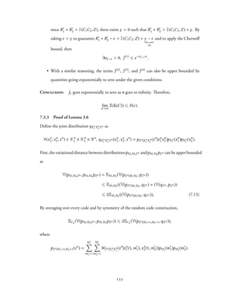
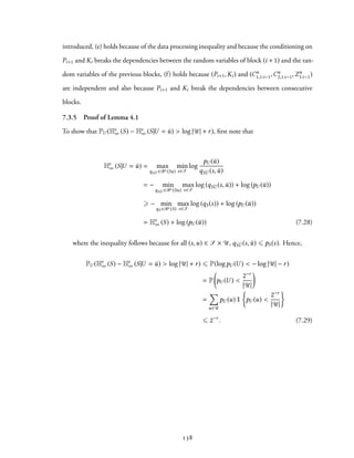
REFERENCES
[1] Abbe, E., “Low complexity constructions of secret keys using polar coding”. In:
Proceedings of the IEEE Information Theory Workshop (ITW). Vol. 36. 2012 (cit. on
p. 122).
[2] Abdi, A., “On the estimation of the K parameter for the Rice fading distribution”.
In: IEEE Communications Letters 5.3 (2001), pp. 92–94 (cit. on p. 86).
[3] Amariucai, G. T., Wei, S., “Secrecy Rates of Binary Wiretapper Channels Using
Feedback Schemes”. In: Proceedings of the 42ⁿd Annual Conference on Information
Sciences and Systems CISS 2008. Mar. 2008, pp. 624–629 (cit. on p. 47).
[4] Andersson, M., “Equivocation of Eve Using Two Edge Type LDPC Codes for the
Binary Erasure Wiretap Channel”. In: Proceedings of the 44th Asilomar Conference
on Signals, Systems and Computers (ASILOMAR). IEEE. 2010, pp. 2045–2049 (cit.
on p. 99).
[5] Ardestanizadeh, E., “Wiretap Channel With Secure Rate-Limited Feedback”. In:
IEEE Transactions on Information Theory 55.12 (Dec. 2009), pp. 5353–5361 (cit.
on p. 47).
[6] Arimoto, S., “Information Measures and Capacity of Order α for Discrete Mem-
oryless Channels”. In: Topics in Information Theory. (Colloquia Mathematica So-
cietatis János Bolyai) 16 (1977), pp. 41–52 (cit. on p. 19).
[7] Arıkan, E., “Channel Polarization: A Method for Constructing Capacity-Achieving
Codes for Symmetric Binary-Input Memoryless Channels”. In: IEEE Transactions
on Information Theory 55.7 (2009), pp. 3051–3073 (cit. on pp. 46, 122).
[8] Barros, J., Bloch, M., “Strong Secrecy for Wireless Channels (Invited Talk)”. In:
Information Theoretic Security. Springer, 2008, pp. 40–53 (cit. on p. 93).
139

[9] Bennett, C. H., “Generalized Privacy Amplification”. In: IEEE Transactions on
Information Theory 41.6 (Nov. 1995), pp. 1915–1923 (cit. on pp. 10, 93).
[10] Bharadia, D., McMilin, E., Katti, S., “Full Duplex Radios”. In: Proceedings of the
ACM SIGCOMM 2013 Conference. Aug. 2013 (cit. on p. 82).
[11] Bloch, M., Laneman, J. N., “On the Secrecy Capacity of Arbitrary Wiretap Chan-
nels”. In: Proceedings of the 46th Allerton Conference on Communication, Control,
and Computing. Monticello, IL, Sept. 2008, pp. 818–825 (cit. on p. 48).
[12] Bloch, M., “Channel Scrambling for Secrecy”. In: Proceedings of the IEEE Interna-
tional Symposium on Information Theory. Seoul, Korea, July 2009, pp. 2452–2456
(cit. on p. 47).
[13] Bloch, M., “Channel Intrinsic Randomness”. In: Proceedings of the IEEE Interna-
tional Symposium on Information Theory. Austin, TX, June 2010, pp. 2607–2611
(cit. on pp. 34, 35, 46).
[14] Bloch, M. R., Kliewer, J., “On Secure Communication with Constrained Ran-
domization”. In: Proceedings of the IEEE International Symposium on Information
Theory (ISIT). Cambridge, MA, July 2012, pp. 1172–1176 (cit. on p. 36).
[15] Bloch, M. R., Luzzi, L., Kliewer, J., “Strong Coordination with Polar Codes”. In:
Proceedings of the 50th Annual Allerton Conference on Communication, Control, and
Computing. 2012, pp. 565–571 (cit. on p. 122).
[16] Bloch, M., Barros, J., Physical-layer Security: from Information Theory to Security
Engineering. Cambridge University Press, 2011 (cit. on pp. xvi, 13, 31, 33, 92,
96).
[17] Bloch, M., Laneman, J., “Strong Secrecy From Channel Resolvability”. In: IEEE
Transactions on Information Theory 59.12 (Dec. 2013), pp. 8077–8098 (cit. on
pp. 5, 7, 85).
140

[18] Cachin, C., Maurer, U. M., “Linking Information Reconciliation and Privacy
Amplification”. In: Journal of Cryptology 10.2 (Mar. 1997), pp. 97–110 (cit. on
p. 81).
[19] Chen, C., Jensen, M., “Secret Key Establishment Using Temporally and Spatially
Correlated Wireless Channel Coefficients”. In: IEEE Transactions on Mobile Com-
puting 10.2 (Feb. 2011), pp. 205–215 (cit. on pp. 75, 85).
[20] Chou, R., Bloch, M., “Secret-Key Generation with Arbitrarily Varying Eavesdrop-
per’s Channel”. In: Proceedings of the IEEE GlobalSIP 2013. 2013 (cit. on pp. 93,
98).
[21] Chou, R., Bloch, M., “Separation of Reliability and Secrecy in Rate-Limited Secret-
Key Generation”. In: IEEE Transactions on Information Theory 60.8 (Aug. 2014),
pp. 4941–4957 (cit. on pp. 80, 93).
[22] Chou, R., Bloch, M., Abbe, E., “Polar Coding for Secret-key Generation”. In:
Proceedings of the 2013 IEEE Information Theory Workshop (ITW). Sept. 2013,
pp. 1–5 (cit. on pp. 99, 120, 122, 123).
[23] Cover, T. M., Thomas, J. A., Elements of Information Theory. 2nd. Wiley-Interscience,
2006 (cit. on pp. xvi, 13, 24, 31, 33, 93).
[24] Csiszàr, I., Narayan, P., “Common Randomness and Secret Key Generation with a
Helper”. In: IEEE Transactions on Information Theory 46.2 (Mar. 2000), pp. 344–
366 (cit. on pp. 47, 58, 69, 80).
[25] Csiszàr, I., Narayan, P., “Secrecy Capacities for Multiple Terminals”. In: IEEE
Transactions on Information Theory 50.12 (Dec. 2004), pp. 3047–3061 (cit. on
p. 8).
[26] Csiszàr, I., Körner, J., Information Theory: Coding Theorems for Discrete Memoryless
Systems. Cambridge University Press, 2011 (cit. on pp. 20, 21, 44).
141

[27] El Gamal, A., Kim, Y.-H., Network Information Theory. Cambridge University
Press, 2011 (cit. on p. 62).
[28] El Gamal, A., “New Achievable Secrecy Rate Regions for the Two-Way Wiretap
Channel”. In: Proceedings of the IEEE Information Theory Workshop. Cairo, Egypt,
Jan. 2010, pp. 1–5 (cit. on pp. 47, 48, 52, 58, 60).
[29] Erven, T., Harremoës, P., “Rényi Divergence and Majorization”. In: Proceedings of
the IEEE International Symposium on Information Theory (ISIT). Austin, TX, June
2010, pp. 1335–1339 (cit. on p. 38).
[30] Erven, T., Harremoës, P., “Rényi Divergence and Kullback-Leibler Divergence”.
In: Information Theory, IEEE Transactions on 60.7 (July 2014), pp. 3797–3820
(cit. on p. 21).
[31] Ettus, M., Universal Software Radio Peripheral (USRP). 2008 (cit. on pp. xvi, 123).
[32] Fano, R. M., Transmission of Information: A Statistical Theory of Communication.
New-York: John Wiley & Sons, Inc., 1961 (cit. on p. 93).
[33] Fehr, S., Berens, S., “On the Conditional Rényi Entropy”. In: IEEE Transactions
on Information Theory 60.11 (Nov. 2014), pp. 6801–6810 (cit. on p. 19).
[34] Friis, H. T., “A note on a Simple Transmission Formula”. In: Proceedings of the
IRE 34.5 (1946), pp. 254–256 (cit. on p. 116).
[35] G. D. Forney, J., “On the Role of MMSE Estimation in Approaching the Information-
Theoretic Limits of Linear Gaussian Channels: Shannon Meets Wiener”. In: Pro-
ceedings of the 41st Annual Allerton Conference on Communication, Control, and
Computing. Monticello, IL, Oct. 2003, pp. 430–439 (cit. on p. 59).
[36] GNU Radio Website. http://www.gnuradio.org. Accessed: Apr 23, 2015
(cit. on p. 123).
142

[37] Gündüz, D., Brown, D. R., Poor, H. V., “Secret Communication with Feedback”.
In: Proceedings of the 2008 International Symposium on Information Theory and its
Applications, ISITA2008. Dec. 2008, pp. 1–6 (cit. on p. 47).
[38] Han, T. S., Information-Spectrum Methods in Information Theory. Springer, 2002
(cit. on pp. 45, 48, 49).
[39] Han, T., Verdú, S., “Approximation Theory of Output Statistics”. In: IEEE Trans-
actions on Information Theory 39.3 (May 1993), pp. 752–772 (cit. on pp. 36, 46,
48).
[40] Hayashi, M., “General Nonasymptotic and Asymptotic Formulas in Channel Re-
solvability and Identification Capacity and their Application to the Wiretap Chan-
nels”. In: IEEE Transactions on Information Theory 52.4 (Apr. 2006), pp. 1562–
1575 (cit. on pp. 38, 48).
[41] Hayashi, M., “Exponential Decreasing Rate of Leaked Information in Universal
Random Privacy Amplification”. In: IEEE Transactions on Information Theory 57.6
(2011), pp. 3989–4001 (cit. on pp. 38, 41, 43).
[42] Hayashi, M., Matsumoto, R., “Secure Multiplex Coding with Dependent and
Non-uniform Multiple Messages”. In: Proceedings of the 50th Annual Allerton Con-
ference on Communication, Control, and Computing. 2012, pp. 954–959 (cit. on
p. 36).
[43] He, X., Yener, A., “Providing Secrecy When the Eavesdropper Channel is Arbi-
trarily Varying: A Case for Multiple Antennas”. In: Proceedings of the 48th Annual
Allerton Conference on Communication, Control, and Computing (Allerton). 2010,
pp. 1228–1235 (cit. on pp. 73, 98).
[44] He, X., Yener, A., “The Role of Channel States in Secret Key Generation”. In:
Proceedings of the 21st International Symposium on Personal Indoor and Mobile Radio
Communications (PIMRC). Sept. 2010, pp. 2681–2686 (cit. on p. 120).
143

[45] He, X., Yener, A., “Secrecy When the Eavesdropper Controls its Channel States”.
In: Proceedings of the 2011 IEEE International Symposium on Information Theory
(ISIT), July 2011, pp. 618–622 (cit. on p. 120).
[46] He, X., Yener, A., “The Role of Feedback in Two-Way Secure Communications”.
In: IEEE Transactions on Information Theory 59.12 (Dec. 2013), pp. 8115–8130
(cit. on pp. 47, 48, 58, 74).
[47] Holenstein, T., Renner, R., “On the Randomness of Independent Experiments”.
In: IEEE Transactions on Information Theory 57.4 (Apr. 2011), pp. 1865–1871
(cit. on p. 94).
[48] Hou, J., Kramer, G., “Informational Divergence Approximations to Product Dis-
tributions”. In: Proceedings of the 13th Canadian Workshop on Information Theory
(CWIT). June 2013, pp. 76–81 (cit. on p. 38).
[49] Imai, H., Kobara, K., Morozov, K., “On the Possibility of Key Agreement Using
Variable Directional Antenna”. In: Proceedings of the 1st Joint Workshop on Infor-
mation Security. 2006, pp. 153–157 (cit. on pp. 10, 75).
[50] Imre, “Almost Independence and Secrecy Capacity”. In: Problems of Information
Transmission 32.1 (Jan. 1996), pp. 40–47 (cit. on p. 20).
[51] Iwamoto, M., Shikata, J., “Information Theoretic Security for Encryption Based
on Conditional Rényi Entropies”. In: Information Theoretic Security. Vol. 8317.
Lecture Notes in Computer Science. Springer International Publishing, 2014,
pp. 103–121 (cit. on p. 19).
[52] Jana, S., “On the Effectiveness of Secret Key Extraction from Wireless Signal
Strength in Real Environments”. In: Proceedings of the 15th International Confer-
ence on Mobile Computing and Networking. 2009, pp. 321–332 (cit. on pp. 75,
80, 97).
144

[53] Jimenez Felstrom, A., Zigangirov, K., “Time-varying Periodic Convolutional Codes
with Low-density Parity-check Matrix”. In: IEEE Transactions on Information The-
ory 45.6 (1999), pp. 2181–2191 (cit. on pp. 99, 104).
[54] Klinc, D., “LDPC Codes for the Gaussian Wiretap Channel”. In: IEEE Transac-
tions on Information Forensics and Security 6.3 (2011), pp. 532–540 (cit. on pp. 99,
109, 115).
[55] Kramer, G., Topics in Multi-User Information Theory. Vol. 4. Foundations and
Trends in Communications and Information Theory 4-5. NOW Publishers, 2008,
pp. 265–444 (cit. on p. 22).
[56] Kudekar, S., Kasai, K., “Spatially Coupled Codes over the Multiple Access Chan-
nel”. In: Proceedings of the IEEE International Symposium on Information Theory.
2011, pp. 2816–2820 (cit. on pp. 104, 106, 108–110, 113).
[57] Kudekar, S., Richardson, T., Urbanke, R., “Threshold Saturation via Spatial Cou-
pling: Why Convolutional LDPC Ensembles Perform So Well over the BEC”. In:
IEEE Transactions on Information Theory 57.2 (Feb. 2011), pp. 803–834 (cit. on
pp. xvi, 99, 104, 106).
[58] Lai, L., El Gamal, H., “The Relay-Eavesdropper Channel: Cooperation for Se-
crecy”. In: IEEE Transactions on Information Theory 54.9 (Sept. 2008), pp. 4005–
4019 (cit. on p. 8).
[59] Lai, L., El Gamal, H., Poor, H. V., “The Wiretap Channel With Feedback: En-
cryption Over the Channel”. In: IEEE Transactions on Information Theory 54.11
(Nov. 2008), pp. 5059–5067 (cit. on p. 47).
[60] Leung-Yan-Cheong, S., “On a Special Class of Wiretap Channels”. In: IEEE Trans-
actions on Information Theory 23.5 (1977), pp. 625–627 (cit. on p. 5).
145

[61] Li, Z., “Securing Wireless Systems via Lower Layer Enforcements”. In: Proceedings
of the 2006 ACM Workshop on Wireless Security. Los Angeles, California, USA, Sept.
2006, pp. 33–42 (cit. on p. 75).
[62] R. Liu and W. Trappe, eds. Securing Wireless Communications at the Physical Layer.
Springer, 2010 (cit. on pp. 8, 51).
[63] Madiseh, M., “Secret Key Extraction in Ultra Wideband Channels for Unsyn-
chronized Radios”. In: Proceedings of the 6th Annual Communication Networks and
Services Research Conference. 2008, pp. 88–95 (cit. on pp. 10, 75).
[64] Mahdavifar, H., Vardy, A., “Achieving the Secrecy Capacity of Wiretap Channels
Using Polar Codes”. In: IEEE Transactions on Information Theory 57.10 (2011),
pp. 6428–6443 (cit. on pp. 7, 99, 122, 123).
[65] Mathur, S., “Radio-telepathy: Extracting a Secret Key From An Unauthenticated
Wireless Channel”. In: Proceedings of the 14th ACM International Conference on
Mobile Computing and Networking. ACM. 2008, pp. 128–139 (cit. on p. 97).
[66] Maurer, U., “Secret Key Agreement by Public Discussion from Common Infor-
mation”. In: IEEE Transactions on Information Theory 39 (1993), pp. 733–742
(cit. on p. 96).
[67] Maurer, U., Wolf, S., “From Weak to Strong Information-theoretic Key Agree-
ment”. In: Proceedings of the 2000 IEEE International Symposium on Information
Theory. 2000, pp. 18– (cit. on pp. 10, 92, 93).
[68] Menezes, A. J., Van Oorschot, P. C., Vanstone, S. A., Handbook of Applied Cryp-
tography. CRC press, 1996 (cit. on p. xvi).
[69] Moon, T. K., Error Correction Coding : Mathematical Methods And Algorithms.
John Wiley & Sons, 2005 (cit. on p. xvi).
[70] Murphy, P., Hunter, C., Welsh, E., Wireless Open-Access Research Platform (WARP).
2008 (cit. on p. xvi).
146

[71] Oggier, F., Mihaljevic, M., “An Information-Theoretic Security Evaluation of a
Class of Randomized Encryption Schemes”. In: IEEE Transactions on Information
Forensics and Security 9.2 (Feb. 2014), pp. 158–168 (cit. on p. 121).
[72] Patwari, N., “High-Rate Uncorrelated Bit Extraction for Shared Secret Key Gener-
ation from Channel Measurements”. In: IEEE Transactions on Mobile Computing
9.1 (2010), pp. 17–30 (cit. on pp. 10, 75).
[73] Peng, H., Long, F., Ding, C., “Feature Selection Based on Mutual Information
Criteria of Max-dependency, Max-relevance, and Min-redundancy”. In: IEEE Trans-
actions on Pattern Analysis and Machine Intelligence 27.8 (2005), pp. 1226–1238
(cit. on p. 85).
[74] Pierrot, A. J., Bloch, M. R., “Joint Channel Intrinsic Randomness and Chan-
nel Resolvability”. In: Proceedings of the 2013 IEEE Information Theory Workshop
(ITW). Sept. 2013, pp. 1–5 (cit. on pp. 10, 12, 13).
[75] Pierrot, A. J., Chou, R. A., Bloch, M. R., “Experimental Aspects of Secret Key
Generation in Indoor Wireless Environments”. In: Proceedings of the 14th Work-
shop on Signal Processing Advances in Wireless Communications (SPAWC). June
2013, pp. 669–673 (cit. on pp. 11, 12, 75).
[76] Pierrot, A. J., Bloch, M. R., “Strongly Secure Communications Over the Two-
Way Wiretap Channel”. In: IEEE Transactions on Information Forensics and Secu-
rity 6.3 (Sept. 2011), pp. 595–605 (cit. on pp. 10, 12, 47).
[77] Pierrot, A. J., Bloch, M. R., “LDPC-Based Coded Cooperative Jamming Codes”.
In: Proceedings of the IEEE Information Theory Workshop. Lausanne, Switzerland,
Sept. 2012, pp. 462–466 (cit. on pp. 11, 12, 99).
[78] Pinsker, M. S., Information and Information Stability of Random Variables and
Processes. Holden Day, 1964 (cit. on pp. 21, 93).
147

[79] Premnath, S. N., “Secret Key Extraction from Wireless Signal Strength in Real
Environments”. In: IEEE Transactions on Mobile Computing 12.5 (May 2013),
pp. 917–930 (cit. on p. 75).
[80] Premnath, S. N., “Efficient High-Rate Secret Key Extraction in Wireless Sensor
Networks Using Collaboration”. In: ACM Transactions on Sensor Networks 11.1
(July 2014), 2:1–2:32 (cit. on p. 75).
[81] Proakis, J. G., Digital Communications. 4th. McGraw-Hill, 2001 (cit. on p. xvi).
[82] Rathi, V., “Rate-equivocation Optimal Spatially Coupled LDPC Codes for the
BEC Wiretap Channel”. In: Proceedings of the Information Theory Proceedings (ISIT),
2011 IEEE International Symposium on. Aug. 2011, pp. 2393–2397 (cit. on p. 99).
[83] Renner, R., Wolf, S., “Smooth Rényi Entropy and Applications”. In: Proceedings
of the 2004 International Symposium on Information Theory (ISIT). 2004 (cit. on
p. 19).
[84] Rényi, A., “On Measures of Entropy and Information”. In: Proceedings of the 4th
Berkeley Symposium on Mathematical Statistics and Probability. Vol. 1. Berkeley,
CA, 1961, pp. 547–561 (cit. on pp. 18, 21).
[85] Richardson, T., Urbanke, R., Modern Coding Theory. Cambridge University Press,
2008 (cit. on pp. 111, 112).
[86] Şaşoğlu, E., Telatar, E., Yeh, E., “Polar Codes for the Two-User Multiple-Access
Channel”. In: IEEE Transactions on Information Theory 59.10 (Oct. 2013), pp. 6583–
6592 (cit. on p. 115).
[87] Şaşoğlu, E., Vardy, A., “A New Polar Coding Scheme for Strong Security on Wire-
tap Channels”. In: Proceedings of the 2013 IEEE International Symposium on Infor-
mation Theory (ISIT). July 2013, pp. 1117–1121 (cit. on p. 123).
[88] Shannon, C. E., “A Mathematical Theory of Communication”. In: The Bell System
Technical Journal 27 (July 1948), pp. 379–423, 623–656 (cit. on p. 28).
148

[89] Slepian, D., Wolf, J. K., “Noiseless Coding of Correlated Information Sources”.
In: IEEE Transactions on Information Theory 19.4 (July 1973), pp. 471–480 (cit.
on pp. 30, 31).
[90] Steinberg, Y., “Resolvability Theory for the Multiple-Access Channel”. In: IEEE
Transactions on Information Theory 44.2 (Mar. 1998), pp. 472–487 (cit. on pp. 48,
53, 62, 131, 132).
[91] Storn, R., Price, K., “Differential Evolution – A Simple and Efficient Heuristic for
Global Optimization over Continuous Spaces”. In: Journal of Global Optimization
11.4 (1997), pp. 341–359 (cit. on p. 115).
[92] Tekin, E., Yener, A., “The General Gaussian Multiple-Access and Two-Way Wire-
tap Channels: Achievable Rates and Cooperative Jamming”. In: IEEE Transactions
on Information Theory 54.6 (June 2008), pp. 2735–2751 (cit. on pp. 8, 47, 48, 52,
55, 57, 61).
[93] Tekin, E., Yener, A., “Correction to: “The Gaussian Multiple Access Wire-Tap
Channel” and “The General Gaussian Multiple Access and Two-Way Wire-Tap
Channels: Achievable Rates and Cooperative Jamming””. In: IEEE Transactions
on Information Theory 56.9 (Sept. 2010), pp. 4762–4763 (cit. on pp. 8, 47, 52,
57, 61).
[94] Tse, D., Viswanath, P., Fundamentals of Wireless Communication. Cambridge Uni-
versity Press, 2005 (cit. on p. 86).
[95] Tyagi, H., Watanabe, S., “A bound for Multiparty Secret Key Agreement and
Implications for a Problem of sSecure Computing”. In: Advances in Cryptology–
EUROCRYPT 2014. Springer, 2014, pp. 369–386 (cit. on p. 92).
[96] Vembu, S., Verdú, S., “Generating Random Bits from An Arbitrary Source: Fun-
damental Limits”. In: IEEE Transactions on Information Theory 41.5 (Sept. 1995),
pp. 1322–1332 (cit. on p. 36).
149

[97] Visweswariah, K., Kulkarni, S. R., Verdu, S., “Separation of Random Number
Generation and Resolvability”. In: IEEE Transactions on Information Theory 46.6
(Sept. 2000), pp. 2237–2241 (cit. on p. 36).
[98] Wallace, J., “Secure Physical Layer Key Generation Schemes: Performance and
Information Theoretic Limits”. In: Proceedings of the IEEE International Conference
on Communications (ICC). 2009, pp. 1–5 (cit. on pp. 10, 75).
[99] Wallace, J., Sharma, R., “Automatic Secret Keys From Reciprocal MIMO Wire-
less Channels: Measurement and Analysis”. In: IEEE Transactions on Information
Forensics and Security 5.3 (2010), pp. 381–392 (cit. on pp. 75, 98).
[100] Wang, Q., Xu, K., Ren, K., “Cooperative Secret Key Generation from Phase Es-
timation in Narrowband Fading Channels”. In: IEEE Journal on Selected Areas in
Communications 30.9 (2012), pp. 1666–1674 (cit. on p. 75).
[101] Wang, Q., “Fast and Scalable Secret Key Generation Exploiting Channel Phase
Randomness in Wireless Networks”. In: Proceedings of the 2011 IEEE INFOCOM.
2011, pp. 1422–1430 (cit. on p. 75).
[102] Watanabe, S., Hayashi, M., “Non-asymptotic Analysis of Privacy Amplification
via Rényi Entropy and Inf-spectral Entropy”. In: Proceedings of the 2013 IEEE
International Symposium on Information Theory (ISIT). Istanbul, Turkey, July 2013,
pp. 2715–2719 (cit. on pp. 43, 92, 93).
[103] Watanabe, S., Oohama, Y., “Secret Key Agreement from Vector Gaussian Sources
by Rate-Limited Public Communication”. In: Proceedings of the IEEE Interna-
tional Symposium on Information Theory. Austin, TX, June 2010, pp. 2597–2601
(cit. on pp. 47, 58, 71, 72).
[104] Weedbrook, C., “Gaussian Quantum Information”. In: Reviews of Modern Physics
84.2 (2012), pp. 621–669 (cit. on p. 81).
150

[105] Wilson, R., Tse, D., Scholtz, R. A., “Channel Identification: Secret Sharing Using
Reciprocity in Ultrawideband Channels”. In: IEEE Transactions on Information
Forensics and Security 2.3 (Sept. 2007), pp. 364–375 (cit. on p. 75).
[106] Wong, C. W., Wong, T. F., Shea, J. M., “LDPC Code Design for the BPSK-
Constrained Gaussian Wiretap channel”. In: Proceedings of the 2011 Globecom
Workshops. Dec. 2011, pp. 898–902 (cit. on pp. 99, 109).
[107] Wyner, A. D., “The Wire-Tap Channel”. In: The Bell System Technical Journal 54.8
(Oct. 1975), pp. 1355–1367 (cit. on pp. 4, 99).
[108] Yassaee, M. H., Aref, M. R., “Multiple Access Wiretap Channels with Strong
Secrecy”. In: Proceedings of the IEEE Information Theory Workshop. Dublin, Ireland,
Sept. 2010 (cit. on p. 53).
[109] Ye, C., “Information-Theoretically Secret Key Generation for Fading Wireless
Channels”. In: IEEE Transactions on Information Forensics and Security 5.2 (2010),
pp. 240–254 (cit. on pp. 10, 75, 97).
[110] Zafer, M., Agrawal, D., Srivatsa, M., “A Note on Information-Theoretic Secret
Key Exchange over Wireless Channels”. In: Proceedings of the 47th Annual Allerton
Conference on Communication, Control, and Computing. 2009, pp. 754–761 (cit.
on p. 10).
[111] Zhang, J., Kasera, S., Patwari, N., “Mobility Assisted Secret Key Generation Us-
ing Wireless Link Signatures”. In: Proceedings of the International Conference on
Computer Communications. 2010, pp. 1–5 (cit. on pp. 10, 75).
151

VITA
Alexandre J. Pierrot received the Diplôme d’Ingénieur from Supélec, Gif-sur-Yvette, France,
in 2011 and the M.Sc. degree in Electrical and Computer Engineering from the Georgia
Institute of Technology, Atlanta, ga, in 2011, where he is currently pursuing the Ph.D.
degree. He is working with Prof. Matthieu R. Bloch in the communication architecture
research group (Arcom) at Georgia Tech. His research interests include physical layer
security, digital communications, and digital signal processing.
152

THESIS.DI.AJP.GM

More Related Content

What's hot

Similar to THESIS.DI.AJP.GM

THESIS.DI.AJP.GM