Download to read offline
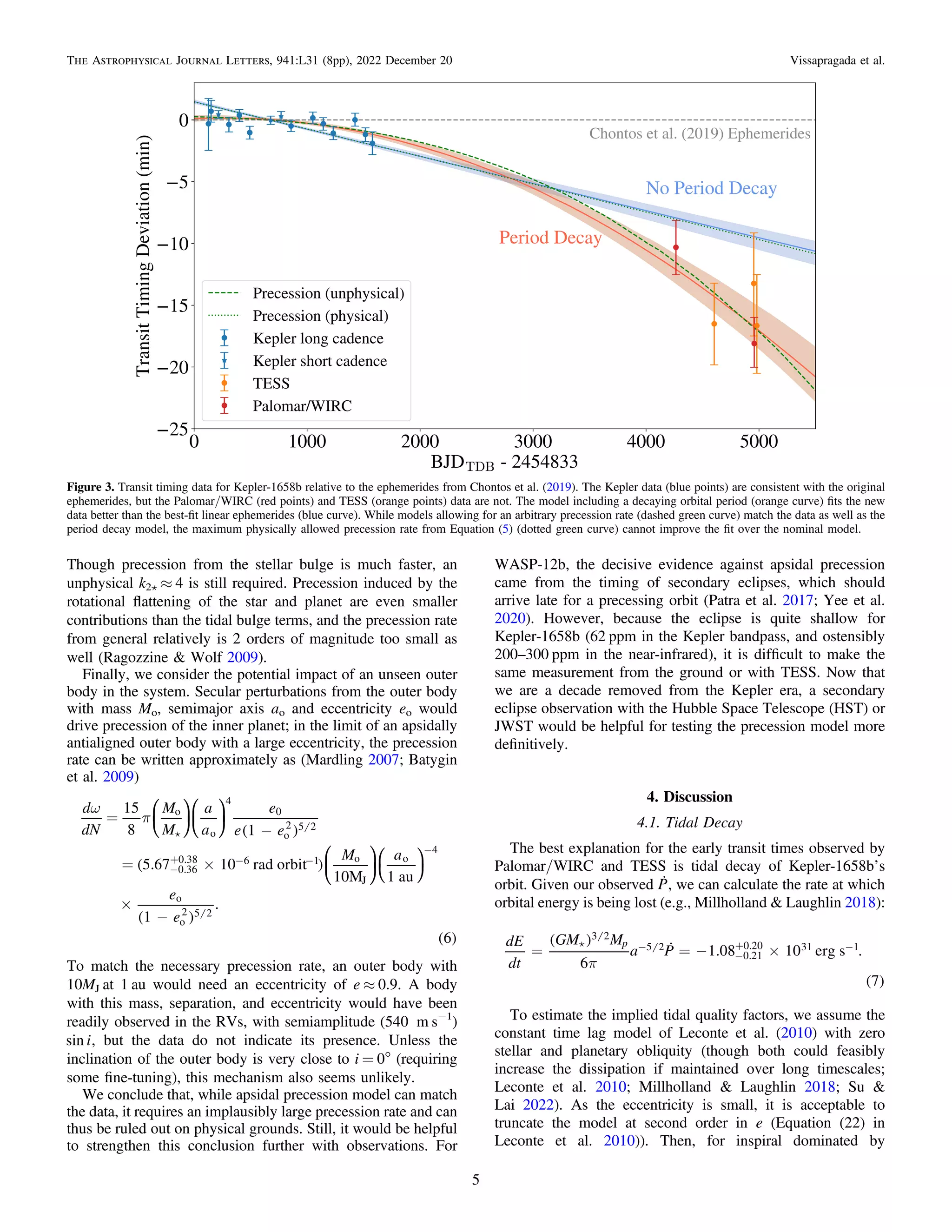

The document presents evidence for tidal-inspired orbital decay in the kepler-1658 system, which includes a giant planet orbiting an evolved star. Measurements show a decreasing orbital period consistent with tidal quality factor predictions, suggesting kepler-1658b exemplifies the effects of tidal interactions before ultimate planetary demise. This finding marks kepler-1658 as a crucial reference for studying tidal physics in exoplanet systems.


