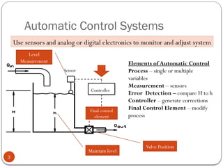
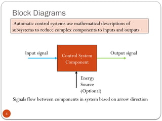
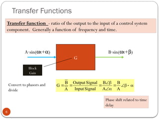
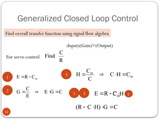
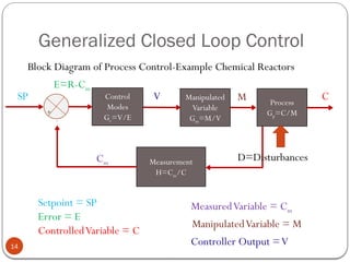
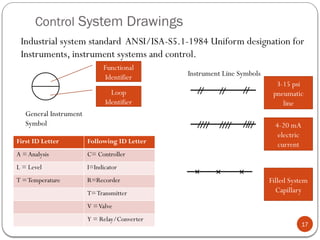
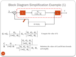
The Control Problem
1
Fundamental Control Concepts
h
Maintain a variable of process at a desired value
while rejecting the effects of outside
disturbances by manipulating another system
variable.
Examples:
Heating and Cooling homes and offices
Automobile cruise control
Hold the position of a mechanical linkage
Maintain level in a tank
Qout depends on h
If Qout = Qin, h constant
Qout > Qin, tank empties
Qout < Qin, tank overflows
Basic Subsystems of Control
2
Feedback Control Subsystems
Measurement
Control decision
System modification
Process-
Maintain tank
level
Measurement-
sight glass
Final Control
Element
Valve
Control Decision
Human adjusts Qout to
maintain h =H
Reference
(setpoint)
h = control
variable
Automatic Control Systems
3
Sensor
Controller
Final control
element
Use sensors and analog or digital electronics to monitor and adjust system
Elements of Automatic Control
Process – single or multiple
variables
Measurement – sensors
Error Detection – compare H to h
Controller – generate corrections
Final Control Element – modify
process
Maintain level
Level
Measurement
Valve Position
Block Diagrams
4
Automatic control systems use mathematical descriptions of
subsystems to reduce complex components to inputs and outputs
Control System
Component
Input signal Output signal
Signals flow between components in system based on arrow direction
Energy
Source
(Optional)
Typical Component Block Diagrams
5
Temperature
Sensor
T (°C)
Vout (mV)
Amplifier
Vin (V)
Vout (V)
Dc Motor
ArmatureV
Va (V)
n (rpm)
Control
Valve
Valve Position
(% Open)
Liquid Flow
(m3
/s)
Level
Transmitter
L (ft)
Current
(mA)
Controller
Error
E (V)
Correction
V (V)
Transfer Functions
6
Transfer function - ratio of the output to the input of a control system
component. Generally a function of frequency and time.
G
A∙sin(wt+a) B∙sin(wt+b)
Convert to phasors and
divide












A
B
A
B
Signal
Input
Signal
Output
A
B
G
Block
Gain
Phase shift related to time
delay
7
Transfer Functions
Examples
Temperature
Sensor
T (°C)
Vout (mV)

mV/C
T
V
Signal
Input
Signal
Output
G out


Example 1-1: Find transfer function of temperature sensor in block diagram
Example 1-2: a current-to-voltage converter takes an input of 17.530° mA and produces
an output of 8.3537° V Determine the transfer function gain and sketch the block diagram.
A
m
V/
7
477
.
0
G
A
m
V/
mA
30
5
.
17
V
37
35
.
8
I
V
Signal
Input
Signal
Output
G
V
37
35
.
8
V
mA
30
5
.
17
I
in
o
o
in

















I-to-V
Converter
G
Iin (mA)
Vout (V)
Open-Loop Control
8
Open loop control modifies output based on predetermined control
values. There is no actual measurement of controlled quantity.
Controller
Final control
element
Control
Valve
Controller
Valve
setting
Output
flow
Tank
Tank
Level
Disturbances
Tank level may vary
with outside
disturbances and
system changes
Closed Loop Control
9
Closed loop control modifies output based on measured values of the
control variable. Measured value compared to desired value and used
to maintain desired value when disturbances occur. Closed loop
control uses feedback of output to input.
Controller
Control
Valve
Tank
Level
Measurement
+
-
Desired
Value
Valve
setting
Output
flow
Measured
level
Tank
Level
Closed Loop Control
10
Example:Auto Cruise Control
Set Speed
Error
Fuel
flow
Controller
Fuel
Injectors
Auto
Speed Sensor
+
-
Engine
Actual
Speed
Mechanical
Power
Disturbances: Up hill/ down hill
Head wind/ tail wind
Disturbances
Generalized Closed Loop Control
11
Block Diagram of Servo Control-Example Positioning Systems
Reference = R
Error = E
ControlledVariable = C
+
-
Controller
G=C/E
Measurement
H=Cm/C
R
Cm
C
E=R-Cm
MeasuredVariable = Cm
Generalized Closed Loop Control
12
Find overall transfer function using signal flow algebra
(Input)(Gain)=(Output)
For servo control
m
C
R
E 

C
G
E
E
C
G 



m
m
C
H
C
C
C
H 



1
2
3
R
C
Find
1 3 m
C
R
E 
 H
C E
C
G
H)
C
R
( 



Overall Transfer Function-Servo Control
13
C
G
H
C
-
G
R
C
G
H)
C
R
(
R
C
Find








R
C
)
H
G
1
(
G
C
)
H
G
1
(
G
R
)
H
G
1
(
C
G
R
G
H
C
C
G
R

















1 2 3
Multiply through by G
Add CHG to both sides
Factor C out of right hand side
Divide both sides by (1+GH)
Divide both sides by R
Generalized Closed Loop Control
14
Block Diagram of Process Control-Example Chemical Reactors
Measurement
H=Cm/C
Manipulated
Variable
Gm=M/V
+
-
Control
Modes
Gc=V/E
Process
Gp=C/M
Setpoint = SP
Error = E
ControlledVariable = C
SP
Cm
C
E=R-Cm
MeasuredVariable = Cm
M
ManipulatedVariable = M
Controller Output =V
V
D=Disturbances
Overall Transfer Function- Process Control
15
Find overall transfer function of process control using signal flow algebra
Series blocks multiple
M
C
G
V
M
G
E
V
G p
m
c 


























M
C
V
M
E
V
G
G
G
G p
m
c







E
C
G
Find overall transfer function Cm/SP C not directly measurable in
process control
16
Overall Transfer Function- Process Control
As before m
C
SP
E 
 C
H
C
C
H
C m
m 



m
m
m
m
m
m
m
m
m
C
H
G
C
SP
H
G
C
C
H
G
SP
H
G
C
)
C
SP
(
H
G
H
C
)
C
SP
(
G
C
)
C
SP
(
G
C
E
G
























SP
C
H
G
1
H
G
C
H
G
1
SP
H
G
)
H
G
1
(
C
SP
H
G
m
m
m















Substitute in for E
Substitute in for C eliminate it
Multiple both sides by H
Multiple L.H. side by GH
Add GHCm to both sides
Factor Cm from right side
Divide both sides by (1+GH)
Divide both sides by SP
Control System Drawings
17
Industrial system standard ANSI/ISA-S5.1-1984 Uniform designation for
Instruments, instrument systems and control.
Functional
Identifier
General Instrument
Symbol
Loop
Identifier
Instrument Line Symbols
3-15 psi
pneumatic
line
4-20 mA
electric
current
Filled System
Capillary
First ID Letter Following ID Letter
A = Analysis C= Controller
L = Level I=Indicator
T =Temperature R=Recorder
T=Transmitter
V =Valve
Y = Relay/Converter
Control System Drawings
18
Heated Product
Heating Fluid
Return
Heating Fluid
Supply
Water
Supply
Syrup
Supply
TIC
102 102
TT
102
TV
LT
LIC
101 101
LY
101
101
LV
103
AT
103
ARC
103
AV
Syrup
Concentration
Current to
Pneumatic
Converter
I/P
Loop 101
Loop 102
Loop 103
101 =level control
102 = temperature control
103 = concentration control
TemperatureTransmitter
Concentration
Valve
Temperature Indicator/Control
Concentration
Recorder/Control
4-20 mA
current
Concentration
Transmitter
Linear and Non-linear Response
19
1 0.5 0 0.5 1
2
0
2
Linear Response
Input
Output
15 10 5 0 5 10 15
2
0
2
Input
Output
Time
Output
Linear transfer functions give proportional
outputs. In this case the factor is 2
Non-linear Response
20
3 2 1 0 1 2 3
10
0
10
Saturation Non-Linearity
Input
Output
15 10 5 0 5 10 15
1
0
1
Input Signal
Saturation Non-Linearity
Time
Input
Signal
15 10 5 0 5 10 15
1
0
1
Output Signal
Saturation Non-Linearity
Time
Output
Signal
Saturation non-linearity typical of practical systems
that have physical limits. Amplifiers, control valves
Other Non-Linearities
21
4 2 0 2 4
2
1
0
1
2
Hystersis Non-Linearity
Input
Output
3 2 1 0 1 2 3
40
20
0
20
40
General Non-Linearity
Input
Output
Typical in magnetic circuit and in
instrumentation transducers
Non-linearities cause distortion in sine waves
response that is not proportional to inputs value
for all signal values.
Block Diagram Simplifications
22
G
H
-
+
R C R C
H
G
1
G
R
C



Block diagram at left simplifies to the above.
Can use this to reduce multiple loops into one
Block.
Also remember that blocks in series multiply
G1 G2 G3 G1G2G3
3
2
1 G
G
G
G 


Equivalent Block
Block Diagram Simplification Example
23
G2
H1
-
+
+
R
-
G1 G3
H3 H2
C
R1
C1
1
2
2
1
1
H
G
1
G
R
C



H
3
2 H
H
H 

Reduce the inner loop
Combine outer feedback block
Combine reduced inner loop with remaining forward gain blocks
Block Diagram Simplification Example (1)
24
+
R
-
G1 G3
H=H2H3
C
1
2
2
H
G
1
G
























1
2
3
2
1
3
1
2
2
1
H
G
1
G
G
G
G
H
G
1
G
G
G Compute the value of G
3
2
1
2
3
2
1
1
2
3
2
1
H
H
H
G
1
G
G
G
1
H
G
1
G
G
G
H
G
1
G
R
C



























Substitute the values of G and H into formula
and simplify
Block Diagram Simplification Example (2)
25
3
2
1
2
3
2
1
1
2
3
2
1
H
H
H
G
1
G
G
G
1
H
G
1
G
G
G
H
G
1
G
R
C



























 
      


























































1
2
3
2
3
2
1
1
2
1
2
3
2
1
1
2
3
2
1
2
3
2
1
1
2
1
2
3
2
1
H
G
1
H
H
G
G
G
H
G
1
H
G
1
G
G
G
H
G
1
H
H
H
G
1
G
G
G
1
H
G
1
H
G
1
G
G
G
R
C
3
2
3
2
1
1
2
3
2
1
H
H
G
G
G
H
G
1
G
G
G
R
C









 Answer
Multiply top and bottom of ratio by (1+G2H1) and simplify
3
2
3
2
1
1
2
3
2
1
H
H
G
G
G
H
G
1
G
G
G









R C
Reduced
block

The Control System engineering designing.pptx

  • 1.
    The Control Problem 1 FundamentalControl Concepts h Maintain a variable of process at a desired value while rejecting the effects of outside disturbances by manipulating another system variable. Examples: Heating and Cooling homes and offices Automobile cruise control Hold the position of a mechanical linkage Maintain level in a tank Qout depends on h If Qout = Qin, h constant Qout > Qin, tank empties Qout < Qin, tank overflows
  • 2.
    Basic Subsystems ofControl 2 Feedback Control Subsystems Measurement Control decision System modification Process- Maintain tank level Measurement- sight glass Final Control Element Valve Control Decision Human adjusts Qout to maintain h =H Reference (setpoint) h = control variable
  • 3.
    Automatic Control Systems 3 Sensor Controller Finalcontrol element Use sensors and analog or digital electronics to monitor and adjust system Elements of Automatic Control Process – single or multiple variables Measurement – sensors Error Detection – compare H to h Controller – generate corrections Final Control Element – modify process Maintain level Level Measurement Valve Position
  • 4.
    Block Diagrams 4 Automatic controlsystems use mathematical descriptions of subsystems to reduce complex components to inputs and outputs Control System Component Input signal Output signal Signals flow between components in system based on arrow direction Energy Source (Optional)
  • 5.
    Typical Component BlockDiagrams 5 Temperature Sensor T (°C) Vout (mV) Amplifier Vin (V) Vout (V) Dc Motor ArmatureV Va (V) n (rpm) Control Valve Valve Position (% Open) Liquid Flow (m3 /s) Level Transmitter L (ft) Current (mA) Controller Error E (V) Correction V (V)
  • 6.
    Transfer Functions 6 Transfer function- ratio of the output to the input of a control system component. Generally a function of frequency and time. G A∙sin(wt+a) B∙sin(wt+b) Convert to phasors and divide             A B A B Signal Input Signal Output A B G Block Gain Phase shift related to time delay
  • 7.
    7 Transfer Functions Examples Temperature Sensor T (°C) Vout(mV)  mV/C T V Signal Input Signal Output G out   Example 1-1: Find transfer function of temperature sensor in block diagram Example 1-2: a current-to-voltage converter takes an input of 17.530° mA and produces an output of 8.3537° V Determine the transfer function gain and sketch the block diagram. A m V/ 7 477 . 0 G A m V/ mA 30 5 . 17 V 37 35 . 8 I V Signal Input Signal Output G V 37 35 . 8 V mA 30 5 . 17 I in o o in                  I-to-V Converter G Iin (mA) Vout (V)
  • 8.
    Open-Loop Control 8 Open loopcontrol modifies output based on predetermined control values. There is no actual measurement of controlled quantity. Controller Final control element Control Valve Controller Valve setting Output flow Tank Tank Level Disturbances Tank level may vary with outside disturbances and system changes
  • 9.
    Closed Loop Control 9 Closedloop control modifies output based on measured values of the control variable. Measured value compared to desired value and used to maintain desired value when disturbances occur. Closed loop control uses feedback of output to input. Controller Control Valve Tank Level Measurement + - Desired Value Valve setting Output flow Measured level Tank Level
  • 10.
    Closed Loop Control 10 Example:AutoCruise Control Set Speed Error Fuel flow Controller Fuel Injectors Auto Speed Sensor + - Engine Actual Speed Mechanical Power Disturbances: Up hill/ down hill Head wind/ tail wind Disturbances
  • 11.
    Generalized Closed LoopControl 11 Block Diagram of Servo Control-Example Positioning Systems Reference = R Error = E ControlledVariable = C + - Controller G=C/E Measurement H=Cm/C R Cm C E=R-Cm MeasuredVariable = Cm
  • 12.
    Generalized Closed LoopControl 12 Find overall transfer function using signal flow algebra (Input)(Gain)=(Output) For servo control m C R E   C G E E C G     m m C H C C C H     1 2 3 R C Find 1 3 m C R E   H C E C G H) C R (    
  • 13.
    Overall Transfer Function-ServoControl 13 C G H C - G R C G H) C R ( R C Find         R C ) H G 1 ( G C ) H G 1 ( G R ) H G 1 ( C G R G H C C G R                  1 2 3 Multiply through by G Add CHG to both sides Factor C out of right hand side Divide both sides by (1+GH) Divide both sides by R
  • 14.
    Generalized Closed LoopControl 14 Block Diagram of Process Control-Example Chemical Reactors Measurement H=Cm/C Manipulated Variable Gm=M/V + - Control Modes Gc=V/E Process Gp=C/M Setpoint = SP Error = E ControlledVariable = C SP Cm C E=R-Cm MeasuredVariable = Cm M ManipulatedVariable = M Controller Output =V V D=Disturbances
  • 15.
    Overall Transfer Function-Process Control 15 Find overall transfer function of process control using signal flow algebra Series blocks multiple M C G V M G E V G p m c                            M C V M E V G G G G p m c        E C G Find overall transfer function Cm/SP C not directly measurable in process control
  • 16.
    16 Overall Transfer Function-Process Control As before m C SP E   C H C C H C m m     m m m m m m m m m C H G C SP H G C C H G SP H G C ) C SP ( H G H C ) C SP ( G C ) C SP ( G C E G                         SP C H G 1 H G C H G 1 SP H G ) H G 1 ( C SP H G m m m                Substitute in for E Substitute in for C eliminate it Multiple both sides by H Multiple L.H. side by GH Add GHCm to both sides Factor Cm from right side Divide both sides by (1+GH) Divide both sides by SP
  • 17.
    Control System Drawings 17 Industrialsystem standard ANSI/ISA-S5.1-1984 Uniform designation for Instruments, instrument systems and control. Functional Identifier General Instrument Symbol Loop Identifier Instrument Line Symbols 3-15 psi pneumatic line 4-20 mA electric current Filled System Capillary First ID Letter Following ID Letter A = Analysis C= Controller L = Level I=Indicator T =Temperature R=Recorder T=Transmitter V =Valve Y = Relay/Converter
  • 18.
    Control System Drawings 18 HeatedProduct Heating Fluid Return Heating Fluid Supply Water Supply Syrup Supply TIC 102 102 TT 102 TV LT LIC 101 101 LY 101 101 LV 103 AT 103 ARC 103 AV Syrup Concentration Current to Pneumatic Converter I/P Loop 101 Loop 102 Loop 103 101 =level control 102 = temperature control 103 = concentration control TemperatureTransmitter Concentration Valve Temperature Indicator/Control Concentration Recorder/Control 4-20 mA current Concentration Transmitter
  • 19.
    Linear and Non-linearResponse 19 1 0.5 0 0.5 1 2 0 2 Linear Response Input Output 15 10 5 0 5 10 15 2 0 2 Input Output Time Output Linear transfer functions give proportional outputs. In this case the factor is 2
  • 20.
    Non-linear Response 20 3 21 0 1 2 3 10 0 10 Saturation Non-Linearity Input Output 15 10 5 0 5 10 15 1 0 1 Input Signal Saturation Non-Linearity Time Input Signal 15 10 5 0 5 10 15 1 0 1 Output Signal Saturation Non-Linearity Time Output Signal Saturation non-linearity typical of practical systems that have physical limits. Amplifiers, control valves
  • 21.
    Other Non-Linearities 21 4 20 2 4 2 1 0 1 2 Hystersis Non-Linearity Input Output 3 2 1 0 1 2 3 40 20 0 20 40 General Non-Linearity Input Output Typical in magnetic circuit and in instrumentation transducers Non-linearities cause distortion in sine waves response that is not proportional to inputs value for all signal values.
  • 22.
    Block Diagram Simplifications 22 G H - + RC R C H G 1 G R C    Block diagram at left simplifies to the above. Can use this to reduce multiple loops into one Block. Also remember that blocks in series multiply G1 G2 G3 G1G2G3 3 2 1 G G G G    Equivalent Block
  • 23.
    Block Diagram SimplificationExample 23 G2 H1 - + + R - G1 G3 H3 H2 C R1 C1 1 2 2 1 1 H G 1 G R C    H 3 2 H H H   Reduce the inner loop Combine outer feedback block Combine reduced inner loop with remaining forward gain blocks
  • 24.
    Block Diagram SimplificationExample (1) 24 + R - G1 G3 H=H2H3 C 1 2 2 H G 1 G                         1 2 3 2 1 3 1 2 2 1 H G 1 G G G G H G 1 G G G Compute the value of G 3 2 1 2 3 2 1 1 2 3 2 1 H H H G 1 G G G 1 H G 1 G G G H G 1 G R C                            Substitute the values of G and H into formula and simplify
  • 25.
    Block Diagram SimplificationExample (2) 25 3 2 1 2 3 2 1 1 2 3 2 1 H H H G 1 G G G 1 H G 1 G G G H G 1 G R C                                                                                               1 2 3 2 3 2 1 1 2 1 2 3 2 1 1 2 3 2 1 2 3 2 1 1 2 1 2 3 2 1 H G 1 H H G G G H G 1 H G 1 G G G H G 1 H H H G 1 G G G 1 H G 1 H G 1 G G G R C 3 2 3 2 1 1 2 3 2 1 H H G G G H G 1 G G G R C           Answer Multiply top and bottom of ratio by (1+G2H1) and simplify 3 2 3 2 1 1 2 3 2 1 H H G G G H G 1 G G G          R C Reduced block