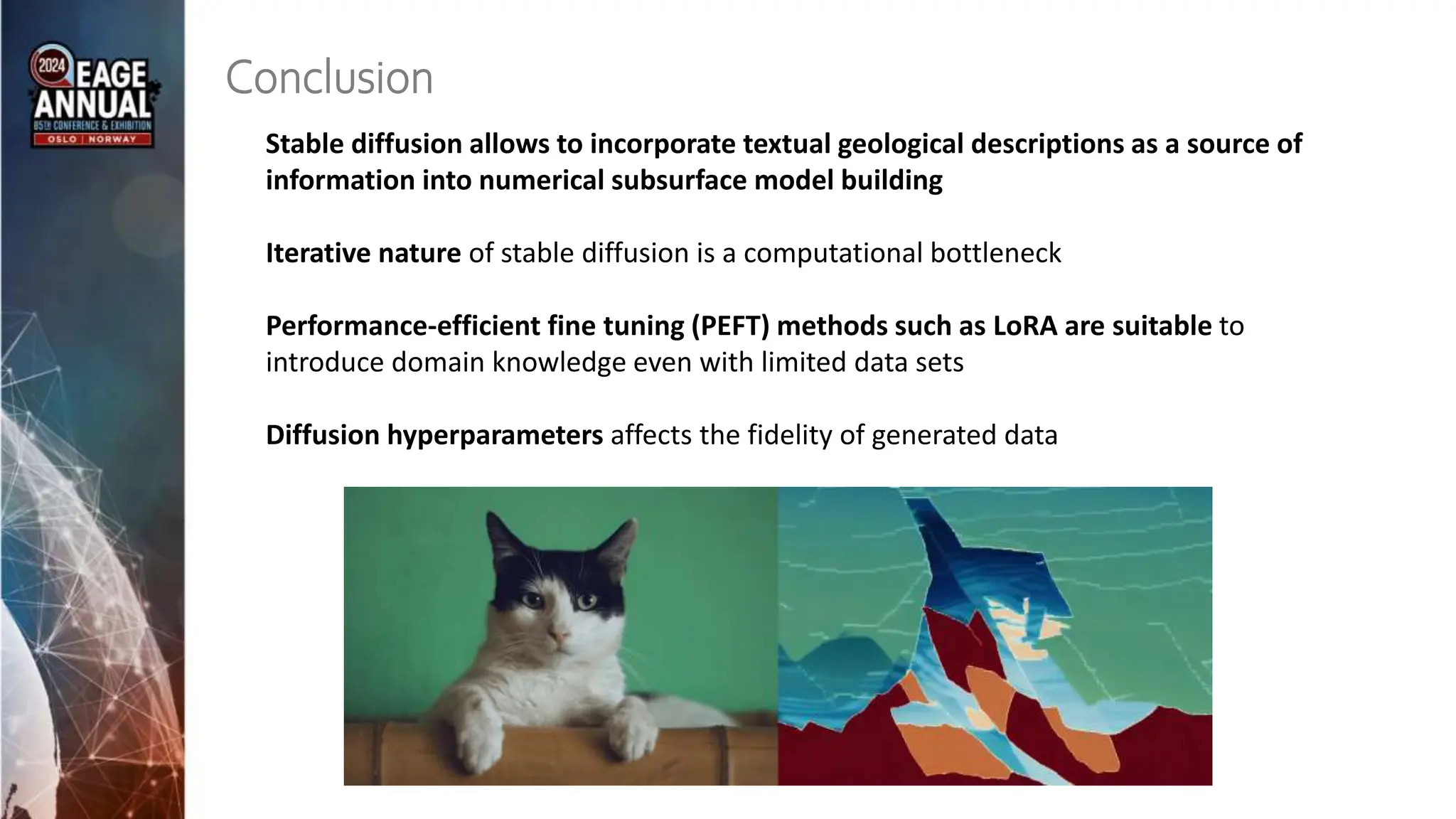
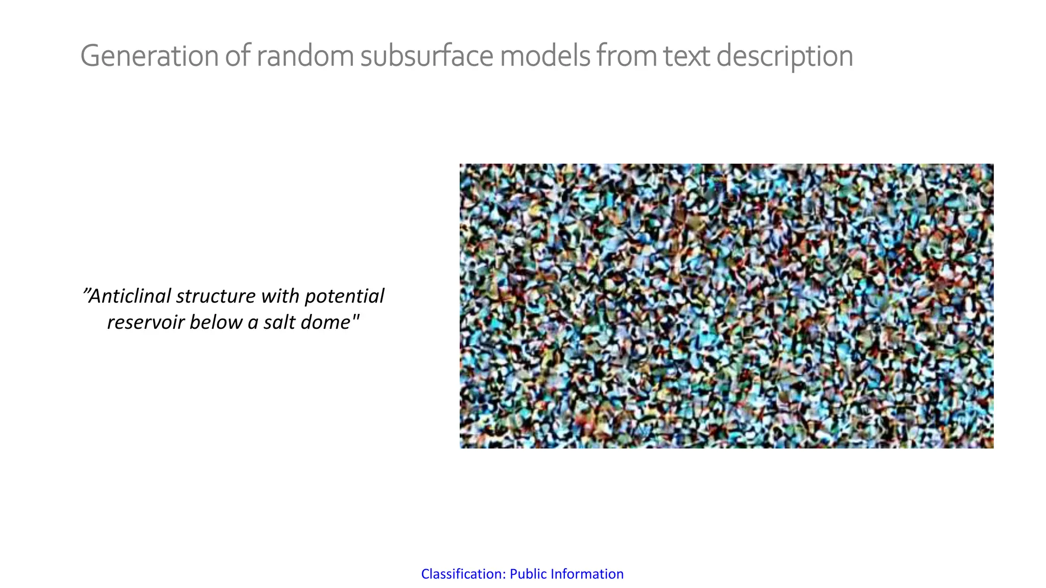
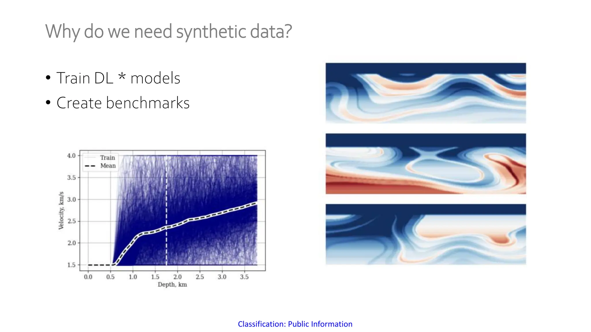
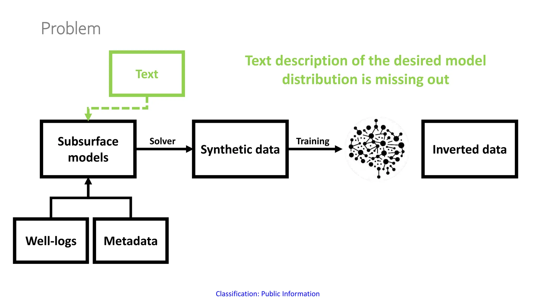
The document discusses a method for generating high-fidelity subsurface models from text descriptions using stable diffusion and low-rank adaptation techniques. It highlights the importance of synthetic data for deep learning model training and the process of merging different modalities to enhance model accuracy. The results suggest that stable diffusion can effectively integrate textual geological information into subsurface model construction, although iterative processes may require performance-efficient tuning methods.


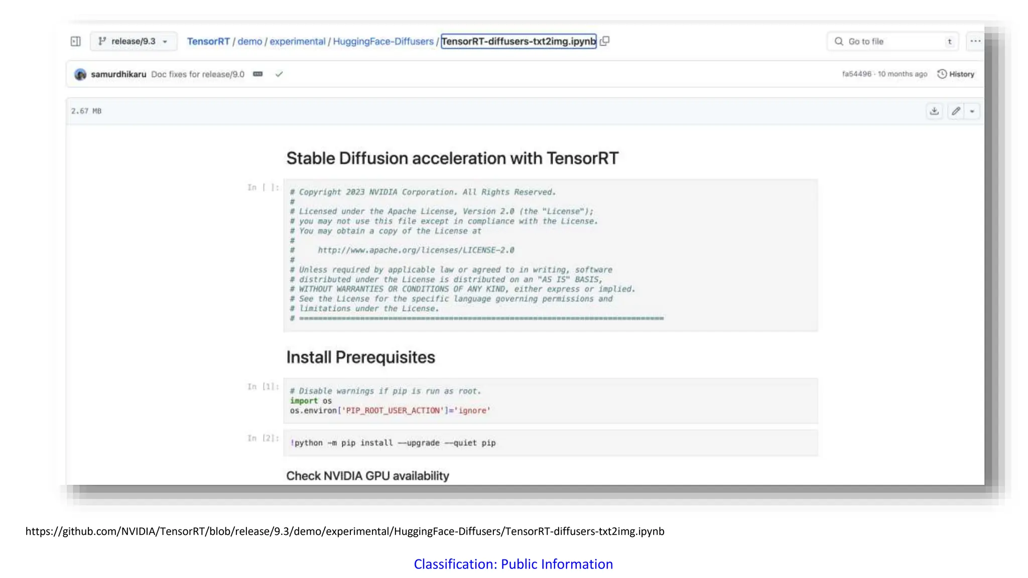
![Classification: Public Information
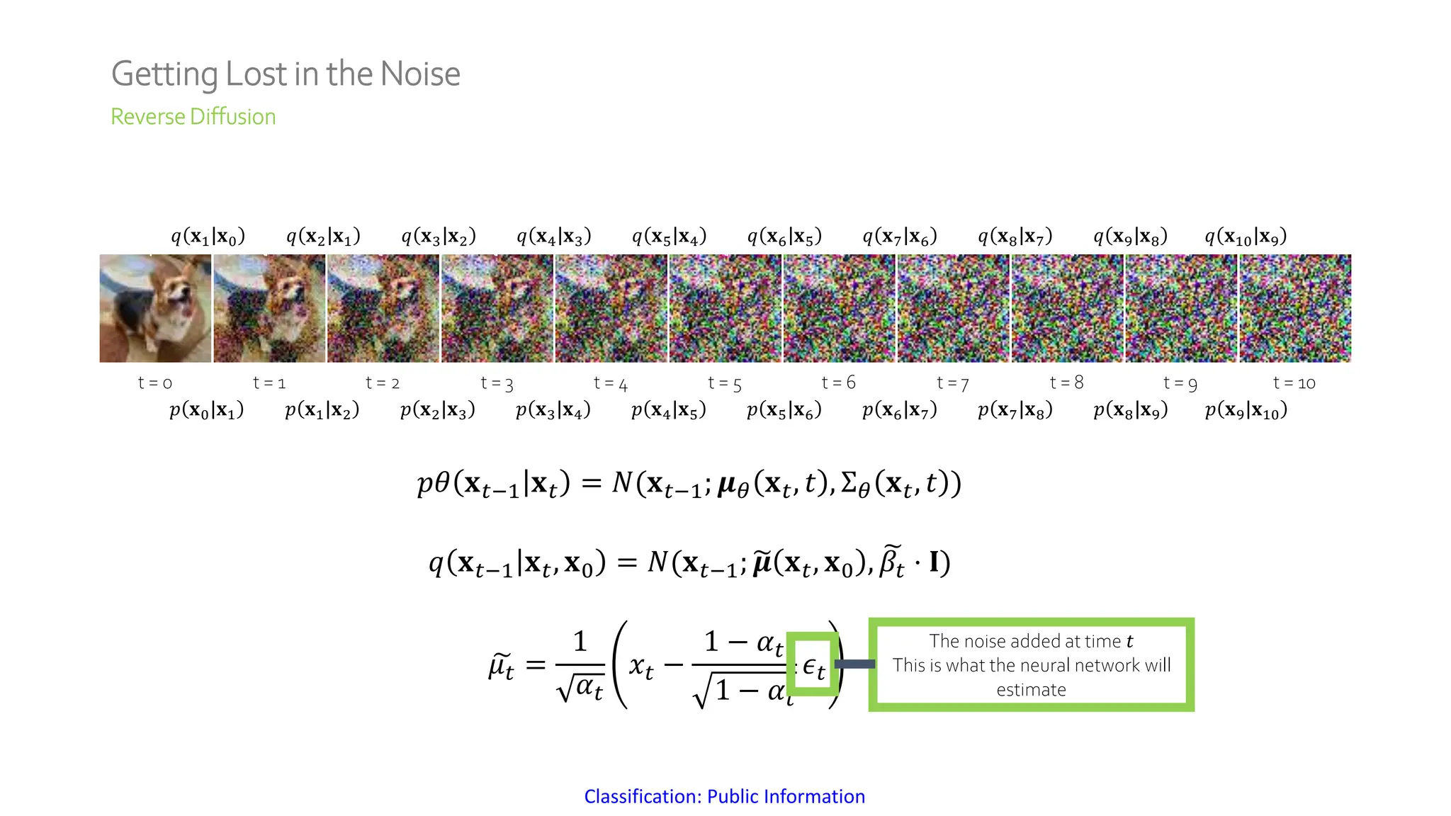
Getting Lost in the Noise
Forward Diffusion
t = 0 t = 1 t = 2 t = 3 t = 4 t = 5 t = 6 t = 7 t = 8 t = 9 t = 10
𝑞 𝐱𝑡 𝐱𝑡−1 = 𝑁(𝐱𝑡; 1 − 𝛽𝑡 ⋅ 𝐱𝑡−1, 𝛽𝑡 ⋅ 𝐈)
• Generate noise from a standard
normal distribution
• Multiply result by 𝛽𝑡
Step1:
• Multiply image at previous step by
1 − 𝛽𝑡
• Add it to the result from step 1
Step2:
noise = torch.randn_like(x_t)
x_t = torch.sqrt(1 - B[t]) * x_t +
torch.sqrt(B[t]) * noise
Code:](https://image.slidesharecdn.com/eage24diffusionudapcompressed-240731063004-8a1deb7e/75/Text-Guided-Well-Log-Constrained-Realistic-Subsurface-Model-Generation-via-Stable-Diffusion-7-2048.jpg)