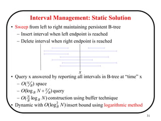
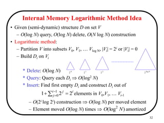
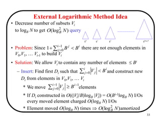
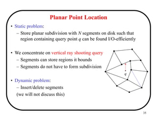
This document discusses temporal databases, which manage both historical and current data, emphasizing the challenges of querying time-varying data in SQL and the benefits of using temporal databases for various applications. It details the concept of intervals and operators on them, as well as introduces persistent B-trees for efficiently managing versions of data. The document concludes with an analysis of persistent B-tree performance for updates and queries while maintaining existence intervals.
![Temporal Databases
S. Srinivasa Rao
April 12, 2007
[Part 1 based on Ch23 of C.J. Date (slides by Prof. Ghafoor, EE 562)]
[Part 2 based on slides by Prof. Arge, I/O-algorithms]](https://image.slidesharecdn.com/temporal-240528223700-f5d4d8d5/85/Temporal-PPT-details-about-the-platform-and-its-uses-1-320.jpg)
![Temporal Databases
S. Srinivasa Rao
April 12, 2007
[Part 1 based on Ch23 of C.J. Date (slides by Prof. Ghafoor, EE 562)]
[Part 2 based on slides by Prof. Arge, I/O-algorithms]](https://image.slidesharecdn.com/temporal-240528223700-f5d4d8d5/75/Temporal-PPT-details-about-the-platform-and-its-uses-1-2048.jpg)
![8
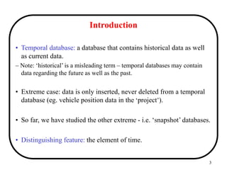
Intervals
• An interval [s,e] is a set of times from time s to time e.
– Does interval [s,e] represent an infinite set?
– Assumption: Timeline is a finite sequence of discrete, indivisible
time quanta.
• Time Quanta: smallest unit of time system can represent.
• Timepoints/point: time unit considered indivisible for our purpose.
• An interval is treated as a single type, not as pair of separate values.
• Interval can be open/closed w.r.t. start point/end point.
– eg. [d04,d10],[d04,d11),(d03,d10],(d03,d11)
all represent the sequence of days from day4 to day10 inclusive.](https://image.slidesharecdn.com/temporal-240528223700-f5d4d8d5/85/Temporal-PPT-details-about-the-platform-and-its-uses-8-320.jpg)
![9
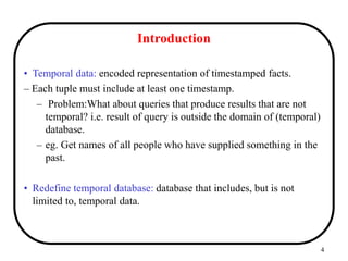
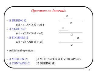
Operators on Intervals
• Temporal predicate operators:
i1 = [s1,e1]; i2 = [s2,e2]
– i1 BEFORE i2
(e1<s2)
– i1 MEETS i2
(s2 = e1)
– i1 EQUALS i2
(s1 = s2 AND e1 = e2)
– i1 OVERLAPS i2
(s2 < s1 < e2 OR s1 < s2 < e1)
i1
i1
i1
i1
i2
i2
i2
i2](https://image.slidesharecdn.com/temporal-240528223700-f5d4d8d5/85/Temporal-PPT-details-about-the-platform-and-its-uses-9-320.jpg)
![11
Scalar and Relational Operators
• DURATION(i) - returns the number of time points in i
– eg. DURATION ([d03,d07]) returns 5
• i1 UNION i2
– returns [MIN(s1,s2),MAX(e1,e2) ]
if (i1 MERGES i2)
otherwise undefined
• i1 INTERSECT i2
– returns [MAX(s1,s2),MIN(e1,e2)]
if (i1 OVERLAPS i2)
otherwise undefined](https://image.slidesharecdn.com/temporal-240528223700-f5d4d8d5/85/Temporal-PPT-details-about-the-platform-and-its-uses-11-320.jpg)
![12
Aggregate Operators
• EXPAND(X):
Where X is a set. The output is also a set.
Used to generate time quantum intervals.
– The expanded form of X is the set of all intervals of the form [p,p]
where p is a time point in some interval in X.
• e.g.:
– X1 = { [d01,d01],[d03,d05],[d04,d06] }
– X2 = { [d01,dp1],[d03,d04],[d05,d05],[d05,d06] }
– X3 = { [d01,d01],[d03,d03],[d04,d04],[d05,d05],[d06,d06] }
– Then EXPAND(X1) = EXPAND(X2) = X3](https://image.slidesharecdn.com/temporal-240528223700-f5d4d8d5/85/Temporal-PPT-details-about-the-platform-and-its-uses-12-320.jpg)
![13
Aggregate Operators
• COLLAPSE(X):
The collapsed form of X is the set Y of intervals of the same type
such that
– (a) X & Y have the same unfolded form.
– (b) no two distinct members i1 and i2 of Y are such that (i1
MERGES i2) is true.
• e.g.:
– X1 = { [d01,d01],[d03,d05],[d04,d06] }
– X2 = { [d01,d01],[d03,d04],[d05,d05],[d05,d06] }
– X3 = { [d01,d01],[d03,d06] }
– Then COLLAPSE (X1) = COLLAPSE (X2) = X3](https://image.slidesharecdn.com/temporal-240528223700-f5d4d8d5/85/Temporal-PPT-details-about-the-platform-and-its-uses-13-320.jpg)
![15
Example
S# P# During
S1 P1 [d04,d10]
S1 P7 [d05,d10]
S1 P3 [d09,d10]
S1 P5 [d06,d10]
S2 P1 [d02,d04]
S2 P9 [d03,d03]
S2 P1 [d08,d10]
S2 P5 [d09,d10]
S3 P1 [d08,d10]
S4 P2 [d06,d09]
S4 P5 [d04,d08]
S4 P7 [d05,d10]
SP
S# During
S1 [d04,d10]
S2 [d02,d04]
S2 [d07,d10]
S3 [d03,d10]
S4 [d04,d10]
S5 [d02,d10]
S
Given two temporal relations:
S: Supplier S# was under contract
during the interval During
SP: Supplier S# was able to supply
part P# during the interval During](https://image.slidesharecdn.com/temporal-240528223700-f5d4d8d5/85/Temporal-PPT-details-about-the-platform-and-its-uses-15-320.jpg)
![16
Example 1
• Active supplier intervals: Get S#-DURING pairs for
suppliers who have been able to supply at least one
part during at least one interval of time, where
DURING designates such an interval.
• PACK SP {S#,DURING} ON DURING
S# P# During
S1 P1 [d04,d10]
S1 P7 [d05,d10]
S1 P3 [d09,d10]
S1 P5 [d06,d10]
S2 P1 [d02,d04]
S2 P9 [d03,d03]
S2 P1 [d08,d10]
S2 P5 [d09,d10]
S3 P1 [d08,d10]
S4 P2 [d06,d09]
S4 P5 [d04,d08]
S4 P7 [d05,d10]
SP
S# During
S1 [d04,d10]
S2 [d02,d04]
S2 [d08,d10]
S3 [d08,d10]
S4 [d04,d10]
RESULT](https://image.slidesharecdn.com/temporal-240528223700-f5d4d8d5/85/Temporal-PPT-details-about-the-platform-and-its-uses-16-320.jpg)
![17
Example 2
• Inactive (passive) supplier intervals: Get S#-DURING pairs for
suppliers who have been unable to supply any parts at all during at
least one interval of time, where DURING designates such an
interval.
• PACK
( ( UNPACK S {S#,DURING} ON DURING )
MINUS
( UNPACK SP {S#,DURING} ON DURING ) )
ON DURING
• Shorthand: U_MINUS
S# During
S2 [d07,d07]
S3 [d03,d07]
S5 [d02,d10]
RESULT](https://image.slidesharecdn.com/temporal-240528223700-f5d4d8d5/85/Temporal-PPT-details-about-the-platform-and-its-uses-17-320.jpg)