Downloaded 16 times
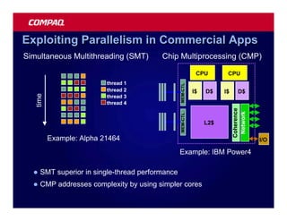
![The End of Moore’s law
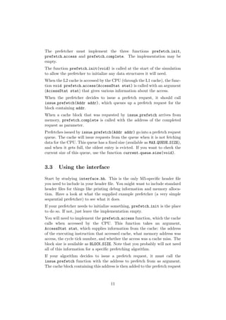
Motivational background
for single-core microprocessors
• Why multicores
– in all market segments from mobile phones to supercomputers
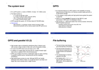
• The ”end” of Moores law
• The power wall
• The memory wall
• The bandwith problem
• ILP limitations
• The complexity wall
But Moore’s law still holds for
FPGA, memory and
multicore processors
13 Lasse Natvig 14 Lasse Natvig
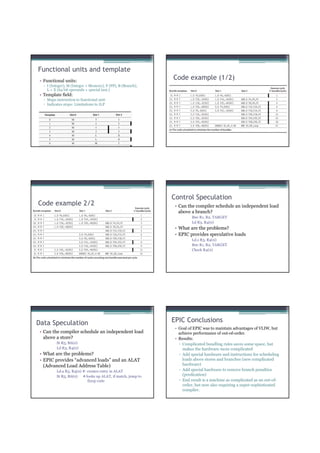
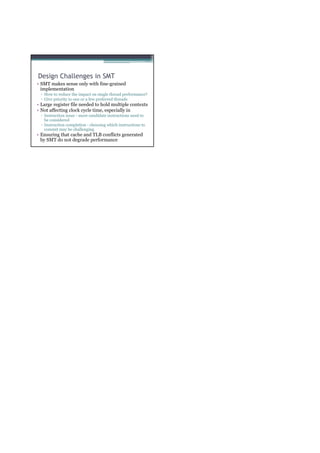
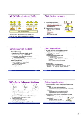
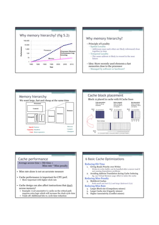
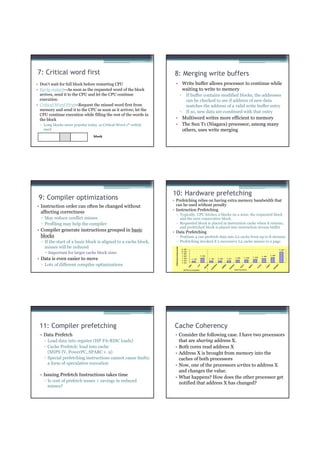
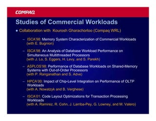
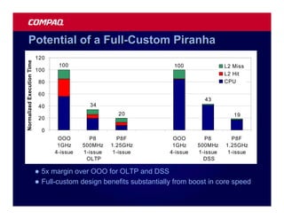
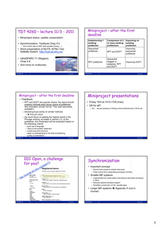
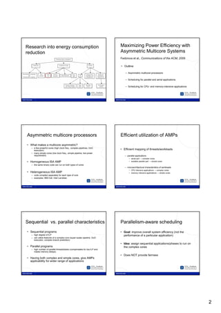
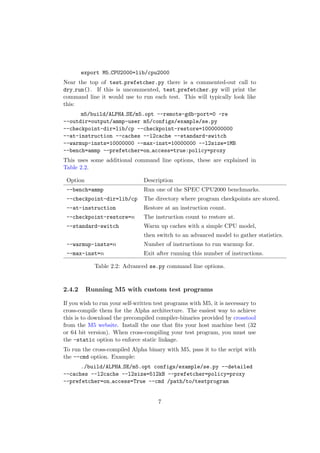
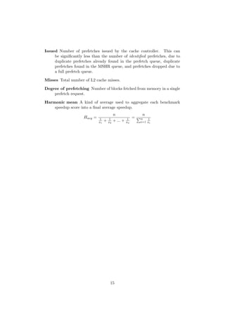
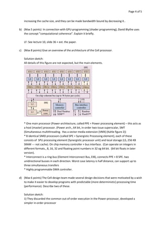
Energy & Heat Problems The Memory Wall
1000
• Large power “Moore’s Law”
consumption 100 CPU
60%/year
– Costly
Performance
P-M gap grows 50% / year
– Heat problems 10
– Restricted battery
DRAM
operation time 9%/year
9%/
1
• Google ”Open
House Trondheim 1980 1990 2000
2006” • The Processor Memory Gap
– ”Performance/Watt
is the only flat
• Consequence: deeper memory hierachies
trend line” – P – Registers – L1 cache – L2 cache – L3 cache – Memory - - -
– Complicates understanding of performance
• cache usage has an increasing influence on performance
15 Lasse Natvig 16 Lasse Natvig
The I/O pin or Bandwidth problem The limitations of ILP
(Instruction Level Parallelism)
• # I/O signaling pins in Applications
– limited by physical
tecnology 30 3
– speeds have not 2.5
25
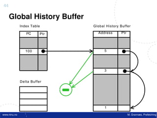
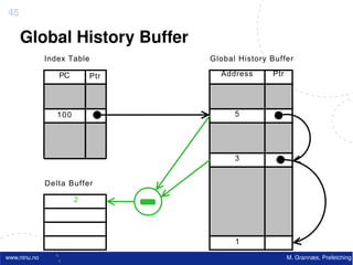
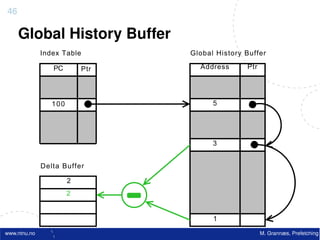
increased at the same
Fraction of total cycles (%)
rate as processor clock 20 2
rates
dup
Speed
1.5
• Projections 15
– from ITRS (International 10 1
Technology Roadmap
for Semiconductors) 5 0.5
0 0
[Huh, Burger and Keckler 2001] 0 1 2 3 4 5 6+ 0 5 10 15
Number of instructions issued Instructions issued per cycle
17 Lasse Natvig 18 Lasse Natvig
3](https://image.slidesharecdn.com/tdt4260-110828142109-phpapp02/85/tdt4260-3-320.jpg)
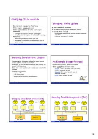
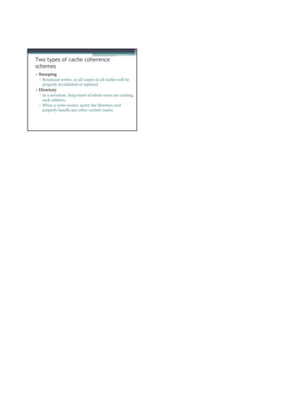
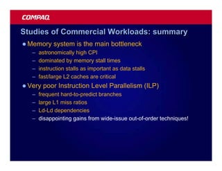
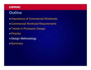
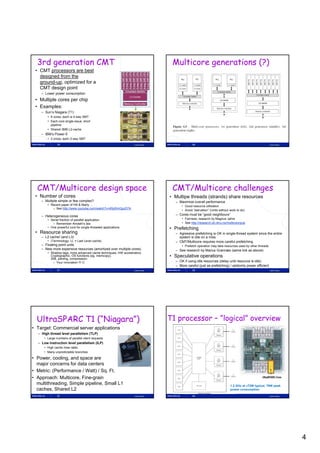
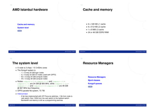
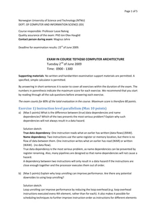
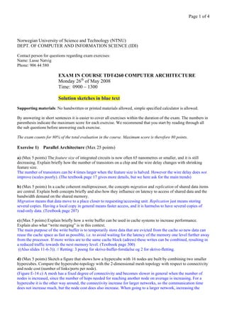
![Reduced Increase in Clock Frequency Solution: Multicore architectures
(also called Chip Multi-processors - CMP)
• More power-efficient
– Two cores with clock frequency f/2
can potentially achieve the same
speed as one at frequency f with 50%
reduction in total energy consumption
[Olukotun & Hammond 2005]
• Exploits Thread Level
Parallelism (TLP)
– in addition to ILP
– requires multiprogramming or
parallel programming
• Opens new possibilities for
architectural innovations
19 Lasse Natvig 20 Lasse Natvig
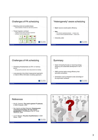
Why heterogeneous multicores? CPU – GPU – convergence
• Specialized HW is (Performance – Programmability)
Cell BE processor
faster than general
HW Processors: Larrabee,
Fermi, …
– Math co-processor Languages: CUDA,
OpenCL, …
– GPU, DSP, etc…
• Benefits of
customization
– Similar to ASIC vs. general
purpose programmable
HW
• Amdahl’s law
– Parallel speedup limited by
serial fraction
• 1 super-core
21 Lasse Natvig 22 Lasse Natvig
Parallel processing – conflicting Multicore programming challenges
goals • Instability, diversity, conflicting goals … what to do?
Performance • What kind of parallel programming?
The P6-model: Parallel Processing – Homogeneous vs. heterogeneous
challenges: Performance, Portability, – DSL vs. general languages
Programmability and Power efficiency – Memory locality
Portability • What to teach?
– Teaching should be founded on
active research
Programmability Powerefficiency • Two layers of programmers
y p g
– The Landscape of Parallel Computing Research: A View from
• Examples; Berkeley [Asan+06]
– Performance tuning may reduce portability • Krste Asanovic presentation at ACACES Summerschool 2007
• Eg. Datastructures adapted to cache block size – 1) Programmability layer (Productivity layer) (80 - 90%)
• ”Joe the programmer”
– New languages for higher programmability may reduce performance
and increase power consumption – 2) Performance layer (Efficiency layer) (10 - 20%)
• Both layers involved in HPC
• Programmability an issue also at the performance-layer
23 Lasse Natvig 24 Lasse Natvig
4](https://image.slidesharecdn.com/tdt4260-110828142109-phpapp02/85/tdt4260-4-320.jpg)
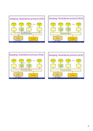
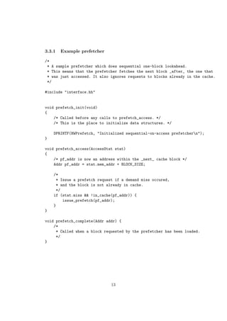
![COST and COTS Speedup Superlinear speedup ?
• Cost • General definition:
Performance (p processors)
– to produce one unit Speedup (p processors) = Performance (1 processor)
– include (development cost / # sold units)
– benefit of large volume
• COTS • For a fixed problem size (input data set),
– commodity off the shelf
dit ff th h lf performance = 1/time
– Speedup
Time (1 processor)
fixed problem (p processors) =
Time (p processors)
• Note: use best sequential algorithm in the uni-processor
solution, not the parallel algorithm with p = 1
37 Lasse Natvig 38 Lasse Natvig
Amdahl’s Law (1967) (fixed problem size) Gustafson’s “law” (1987)
(scaled problem size, fixed execution time)
• “If a fraction s of a
(uniprocessor) • Total execution time on
computation is inherently parallel computer with n
serial, the speedup is at processors is fixed
most 1/s” – serial fraction s’
• Total work in computation – parallel fraction p’
– serial fraction s – s’ + p’ = 1 (100%)
– parallel fraction p
p • S (n) Time’(1)/Time’(n)
S’(n) = Time (1)/Time (n)
– s + p = 1 (100%)
= (s’ + p’n)/(s’ + p’)
• S(n) = Time(1) / Time(n) = s’ + p’n = s’ + (1-s’)n
= (s + p) / [s +(p/n)] = n +(1-n)s’
• Reevaluating Amdahl's law,
= 1 / [s + (1-s) / n] John L. Gustafson, CACM May
1988, pp 532-533. ”Not a new
= n / [1 + (n - 1)s] law, but Amdahl’s law with
changed assumptions”
• ”pessimistic and famous”
39 Lasse Natvig 40 Lasse Natvig
How the serial fraction limits speedup
• Amdahl’s law
• Work hard to
reduce the
serial part of
the application
– remember IO
– think different
(than traditionally = serial fraction
or sequentially)
41 Lasse Natvig
7](https://image.slidesharecdn.com/tdt4260-110828142109-phpapp02/85/tdt4260-7-320.jpg)


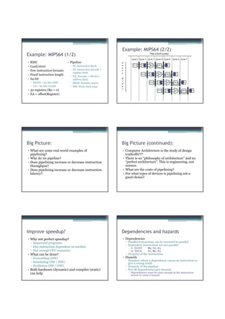
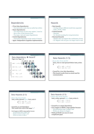
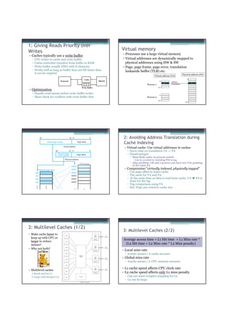
![Example
• Assume branch conditionals are evaluated in the EX
Dynamic scheduling
stage, and determine the fetch address for the following
cycle. • So far: Static scheduling
• If we always stall, how many cycles are bubbled? ▫ Instructions executed in program order
• Assume branch not taken, how many bubbles for an ▫ Any reordering is done by the compiler
incorrect assumption?
• Is stalling on every branch ok? • Dynamic scheduling
• What optimizations could be done to improve stall ▫ CPU reorders to get a more optimal order
penalty? Fewer hazards, fewer stalls, ...
▫ Must preserve order of operations where
reordering could change the result
▫ Covered by TDT 4255 Hardware design
Example
Compiler techniques for ILP Source code: Notice:
for (i = 1000; i >0; i=i-1) • Lots of dependencies
• For a given pipeline and superscalarity • No dependencies between iterations
x[i] = x[i] + s;
▫ How can these be best utilized? • High loop overhead
▫ As few stalls from hazards as possible Loop unrolling
• Dynamic scheduling MIPS:
▫ Tomasulo’s algorithm etc. (TDT4255) Loop: L.D F0,0(R1) ; F0 = x[i]
▫ Makes the CPU much more complicated ADD.D F4,F0,F2 ; F2 = s
• What can be done by the compiler? S.D F4,0(R1) ; Store x[i] + s
▫ Has ”ages” to spend, but less knowledge DADDUI R1,R1,#-8 ; x[i] is 8 bytes
▫ Static scheduling, but what else? BNE R1,R2,Loop ; R1 = R2?
Loop: L.D F0,0(R1)
Static scheduling Loop unrolling ADD.D F4,F0,F2
S.D F4,0(R1)
Loop: L.D F0,0(R1) Loop: L.D F0,0(R1) Loop: L.D F0,0(R1) L.D F6,-8(R1)
stopp DADDUI R1,R1,#-8 ADD.D F4,F0,F2 ADD.D F8,F6,F2
ADD.D F4,F0,F2 ADD.D F4,F0,F2 S.D F4,0(R1) S.D F8,-8(R1)
stopp stopp DADDUI R1,R1,#-8 L.D F10,-16(R1)
stopp stopp BNE R1,R2,Loop ADD.D F12,F10,F2
S.D F4,0(R1) S.D F4,8(R1) S.D F12,-16(R1)
DADDUI R1,R1,#-8 BNE R1,R2,Loop
L.D F14,-24(R1)
stopp • Reduced loop overhead
ADD.D F16,F14,F2
BNE R1,R2,Loop • Requires number of iterations S.D F16,-24(R1)
divisible by n (here n=4)
DADDUI R1,R1,#-32
• Register renaming BNE R1,R2,Loop
• Offsets have changed
Result: From 9 cycles per iteration to 7 • Stalls not shown
(Delays from table in figure 2.2)](https://image.slidesharecdn.com/tdt4260-110828142109-phpapp02/85/tdt4260-19-320.jpg)
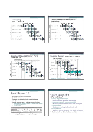
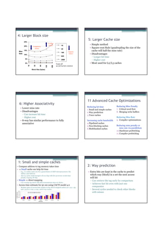
![Loop: L.D F0,0(R1)
Recall: L.D F6,-8(R1)
Loop Unrolling in VLIW
Unrolled Loop L.D
L.D
F10,-16(R1)
F14,-24(R1)
Memory Memory FP FP Int. op/ Clock
reference 1 reference 2 operation 1 op. 2 branch
that minimizes ADD.D F4,F0,F2 L.D F0,0(R1) L.D F6,-8(R1) 1
ADD.D F8,F6,F2 L.D F10,-16(R1) L.D F14,-24(R1) 2
stalls for Scalar ADD.D F12,F10,F2 L.D F18,-32(R1) L.D F22,-40(R1) ADD.D F4,F0,F2 ADD.D F8,F6,F2 3
L.D F26,-48(R1) ADD.D F12,F10,F2 ADD.D F16,F14,F2 4
ADD.D F16,F14,F2
Source code: ADD.D F20,F18,F2 ADD.D F24,F22,F2 5
S.D F4,0(R1) S.D 0(R1),F4 S.D -8(R1),F8 ADD.D F28,F26,F2 6
for (i = 1000; i >0; i=i-1) S.D -16(R1),F12 S.D -24(R1),F16 7
S.D F8,-8(R1)
x[i] = x[i] + s; S.D -32(R1),F20 S.D -40(R1),F24 DSUBUI R1,R1,#48 8
DADDUI R1,R1,#-32
S.D -0(R1),F28 BNEZ R1,LOOP 9
S.D F12,-16(R1)
Register mapping: Unrolled 7 iterations to avoid delays
S.D F16,-24(R1)
7 results in 9 clocks, or 1.3 clocks per iteration (1.8X)
s F2 BNE R1,R2,Loop
Average: 2.5 ops per clock, 50% efficiency
i R1 Note: Need more registers in VLIW (15 vs. 6 in SS)
Problems with 1st Generation VLIW VLIW Tradeoffs
• Increase in code size • Advantages
▫ Loop unrolling ▫ “Simpler” hardware because the HW does not have to
▫ Partially empty VLIW identify independent instructions.
• Operated in lock-step; no hazard detection HW • Disadvantages
▫ A stall in any functional unit pipeline causes entire processor to ▫ Relies on smart compiler
stall, since all functional units must be kept synchronized
▫ Code incompatibility between generations
▫ Compiler might predict function units, but caches hard to predict
▫ There are limits to what the compiler can do (can’t move
▫ Moder VLIWs are “interlocked” (identify dependences between
loads above branches, can’t move loads above stores)
bundles and stall).
• Binary code compatibility
• Common uses
▫ Strict VLIW => different numbers of functional units and unit ▫ Embedded market where hardware simplicity is
latencies require different versions of the code important, applications exhibit plenty of ILP, and binary
compatibility is a non-issue.
IA-64 and EPIC Instruction bundle (VLIW)
• 64 bit instruction set architecture
▫ Not a CPU, but an architecture
▫ Itanium and Itanium 2 are CPUs
based on IA-64
• Made by Intel and Hewlett-Packard (itanium 2 and 3
designed in Colorado)
• Uses EPIC: Explicitly Parallel Instruction Computing
• Departure from the x86 architecture
• Meant to achieve out-of-order performance with in-
order HW + compiler-smarts
▫ Stop bits to help with code density
▫ Support for control speculation (moving loads above
branches)
▫ Support for data speculation (moving loads above stores)
Details in Appendix G.6](https://image.slidesharecdn.com/tdt4260-110828142109-phpapp02/85/tdt4260-22-320.jpg)
![Amdahl’s Law (1967) (fixed problem size) Gustafson’s “law” (1987)
(scaled problem size, fixed execution time)
• “If a fraction s of a
(uniprocessor) • Total execution time on
computation is inherently parallel computer with n
serial, the speedup is at processors is fixed
most 1/s” – serial fraction s’
• Total work in computation – parallel fraction p’
– serial fraction s – s’ + p’ = 1 (100%)
– parallel fraction p
p • S (n) Time’(1)/Time’(n)
S’(n) = Time (1)/Time (n)
– s + p = 1 (100%)
= (s’ + p’n)/(s’ + p’)
• S(n) = Time(1) / Time(n) = s’ + p’n = s’ + (1-s’)n
= (s + p) / [s +(p/n)] = n +(1-n)s’
• Reevaluating Amdahl's law,
= 1 / [s + (1-s) / n] John L. Gustafson, CACM May
1988, pp 532-533. ”Not a new
= n / [1 + (n - 1)s] law, but Amdahl’s law with
changed assumptions”
• ”pessimistic and famous”
13 Lasse Natvig 14 Lasse Natvig
How the serial fraction limits speedup
Single/ILP Multi/TLP
• Uniprocessor trends
• Amdahl’s law – Getting too complex
– Speed of light
– Diminishing returns from ILP
• Work hard to • Multiprocessor
reduce the – Focus in the textbook: 4-32 CPUs
serial part of – Increased performance through parallelism
– Multichip
the application
– Multicore ((Single) Chip Multiprocessors – CMP)
– remember IO
– Cost effective
– think different
(than traditionally = serial fraction • Right balance of ILP and TLP is unclear today
or sequentially) – Desktop vs. server?
15 Lasse Natvig 16 Lasse Natvig
Other Factors Multiprocessor – Taxonomy
Multiprocessors • Flynn’s taxonomy (1966, 1972)
• Growth in data-intensive applications – Taxonomy = classification
– Databases, file servers, multimedia, … – Widely used, but perhaps a bit coarse
• Growing interest in servers, server performance • Single Instruction Single Data (SISD)
• Increasing desktop performance less important – Common uniprocessor
– Outside of graphics
• Si l I t ti M lti l Data (SIMD)
Single Instruction Multiple D t
• Improved understanding in how to use – “ = Data Level Parallelism (DLP)”
multiprocessors effectively
– Especially in servers where significant natural TLP
• Multiple Instruction Single Data (MISD)
– Not implemented?
• Advantage of leveraging design investment by
replication – Pipeline / Stream processing / GPU ?
– Rather than unique design • Multiple Instruction Multiple Data (MIMD)
• Power/cooling issues multicore – Used today
– “ = Thread Level Parallelism (TLP)”
17 Lasse Natvig 18 Lasse Natvig
3](https://image.slidesharecdn.com/tdt4260-110828142109-phpapp02/85/tdt4260-30-320.jpg)


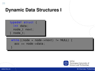
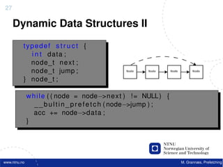
![22
Software Prefetching
f o r ( i =0; i < 10000; i ++) {
acc += data [ i ] ;
}
www.ntnu.no M. Grannæs, Prefetching](https://image.slidesharecdn.com/tdt4260-110828142109-phpapp02/85/tdt4260-70-320.jpg)
![22
Software Prefetching
f o r ( i =0; i < 10000; i ++) {
acc += data [ i ] ;
}
MOV r1, 0 ; Acc
MOV rO, #0 ; i
Label: LOAD r2, r0(#data) ; Cache miss! (400 cycles!)
ADD r1, r2 ; acc += date[i]
INC r0 ; i++
CMP r0, #100000 ; i < 100000
BL Label ; branch if less
www.ntnu.no M. Grannæs, Prefetching](https://image.slidesharecdn.com/tdt4260-110828142109-phpapp02/85/tdt4260-71-320.jpg)
![23
Software Prefetching II
f o r ( i =0; i < 10000; i ++) {
acc += data [ i ] ;
}
Simple optimization using __builtin_prefetch()
f o r ( i =0; i < 10000; i ++) {
_ _ b u i l t i n _ p r e f e t c h (& data [ i + 1 0 ] ) ;
acc += data [ i ] ;
}
www.ntnu.no M. Grannæs, Prefetching](https://image.slidesharecdn.com/tdt4260-110828142109-phpapp02/85/tdt4260-72-320.jpg)
![23
Software Prefetching II
f o r ( i =0; i < 10000; i ++) {
acc += data [ i ] ;
}
Simple optimization using __builtin_prefetch()
f o r ( i =0; i < 10000; i ++) {
_ _ b u i l t i n _ p r e f e t c h (& data [ i + 1 0 ] ) ;
acc += data [ i ] ;
}
Why add 10 (and not 1?)
Prefetch Distance - Memory latency >> Computation latency.
www.ntnu.no M. Grannæs, Prefetching](https://image.slidesharecdn.com/tdt4260-110828142109-phpapp02/85/tdt4260-73-320.jpg)
![24
Software Prefetching III
f o r ( i =0; i < 10000; i ++) {
_ _ b u i l t i n _ p r e f e t c h (& data [ i + 1 0 ] ) ;
acc += data [ i ] ;
}
Note:
• data[0] → data[9] will not be prefetched.
• data[10000] → data[10009] will be prefetched, but not used.
www.ntnu.no M. Grannæs, Prefetching](https://image.slidesharecdn.com/tdt4260-110828142109-phpapp02/85/tdt4260-74-320.jpg)
![24
Software Prefetching III
f o r ( i =0; i < 10000; i ++) {
_ _ b u i l t i n _ p r e f e t c h (& data [ i + 1 0 ] ) ;
acc += data [ i ] ;
}
Note:
• data[0] → data[9] will not be prefetched.
• data[10000] → data[10009] will be prefetched, but not used.
G 9990
Accuracy = = = 0.999 = 99, 9%
G+B 10000
G 9990
Coverage = = = 0.999 = 99, 9%
M 10000
www.ntnu.no M. Grannæs, Prefetching](https://image.slidesharecdn.com/tdt4260-110828142109-phpapp02/85/tdt4260-75-320.jpg)
![25
Complex Software
f o r ( i =0; i < 10000; i ++) {
_ _ b u i l t i n _ p r e f e t c h (& data [ i + 1 0 ] ) ;
i f ( someFunction ( i ) == True )
{
acc += data [ i ] ;
}
}
Does prefetching pay off in this case?
www.ntnu.no M. Grannæs, Prefetching](https://image.slidesharecdn.com/tdt4260-110828142109-phpapp02/85/tdt4260-76-320.jpg)
![25
Complex Software
f o r ( i =0; i < 10000; i ++) {
_ _ b u i l t i n _ p r e f e t c h (& data [ i + 1 0 ] ) ;
i f ( someFunction ( i ) == True )
{
acc += data [ i ] ;
}
}
Does prefetching pay off in this case?
• How many times is someFunction(i) true?
• How much memory bus access is perfomed in
someFunction(i)?
• Does power matter?
We have to profile the program to know!
www.ntnu.no M. Grannæs, Prefetching](https://image.slidesharecdn.com/tdt4260-110828142109-phpapp02/85/tdt4260-77-320.jpg)


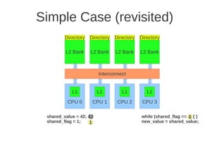
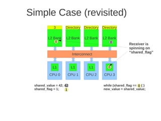
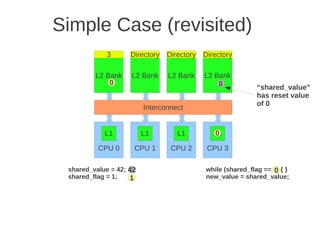
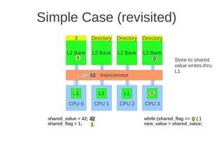
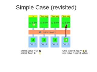
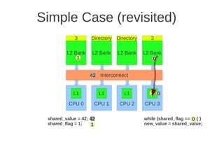
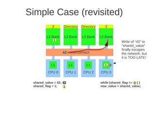
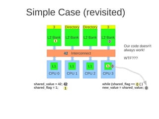
![Atomic exchange (swap) Implementing atomic exchange (1/2)
• Swaps value in register for value in memory • One alternative: Load Linked (LL) and
– Mem = 0 means not locked, Mem = 1 means locked Store Conditional (SC)
– How does this work – Used in sequence
• Register <= 1 ; Processor want to lock • If memory location accessed by LL changes, SC fails
• Exchange(Register, Mem)
• If context switch between LL and SC SC fails
SC,
– If Register = 0 Success
• Mem was = 0 Was unlocked
– Implemented using a special link register
• Mem is now = 1 Now locked • Contains address used in LL
– If Register = 1 Fail • Reset if matching cache block is invalidated or if we get
• Mem was = 1 Was locked an interrupt
• Mem is now = 1 Still locked • SC checks if link register contains the same address. If
• Exchange must be atomic! so, we have atomic execution of LL & SC
7 Lasse Natvig 8 Lasse Natvig
Barrier sync. in BSP
Implementing atomic exchange (2/2) • The BSP-model
• Example code EXCH (R4, 0(R1)): – Leslie G. Valiant, A
bridging model for
try: MOV R3, R4 ; mov exchange value
parallel computation,
LL R2, 0(R1) ; load linked [CACM 1990]
SC R3, 0(R1) ; store conditional – Computations
BEQZ R3, try ; branch if SC failed organised in
MOV R4, R2 ; put load value in R4 supersteps
– Algorithms adapt to
compute platform
• This can now be used to implement e.g. spin locks represented through 4
DADDUI R2, R0, #1 ; R0 always = 0 parameters
lockit: EXCH R2, 0(R1) ; atomic exchange – Helps the combination
BNEZ R2, lockit ; already locked? of portability &
performance
http://www.seas.harvard.edu/news-events/press-releases/valiant_turing
9 Lasse Natvig 10 Lasse Natvig
Multicore Why multicores?
• Important and early example: UltraSPARC T1
• Motivation (See lecture 1)
– In all market segments from mobile phones to supercomputers
– End of Moores law for single-core
– The power wall
– The
Th memory wall ll
– The bandwith problem
– ILP limitations
– The complexity wall
11 Lasse Natvig 12 Lasse Natvig
2](https://image.slidesharecdn.com/tdt4260-110828142109-phpapp02/85/tdt4260-216-320.jpg)
![Chip Multithreading
Opportunities and challenges
• Paper by Spracklen & Abraham, HPCA-11 (2005)
[SA05]
• CMT processors = Chip Multi-Threaded processors
• A spectrum of processor architectures
– Uni-processors with SMT (one core)
– (pure) Chip Multiprocessors (CMP) (one thread pr. core)
– Combination of SMT and CMP (They call it CMT)
• Best suited to server workloads (with high TLP)
13 Lasse Natvig 14 Lasse Natvig
Offchip Bandwidth Sharing processor resources
• SMT
• A bottleneck – Hardware strand
• ”HW for storing the state of a thread of execution”
• Bandwidth increasing, but also latency [Patt04] • Several strands can share resources within the core, such as execution
resources
• Need more than 100 in-flight requests to fully utilize – This improves utilization of processor resources
the available bandwidth – Reduces applications sensitivity to off-chip misses
• Switch between threads can be very efficient
• (pure) CMP
– Multiple cores can share chip resources such as memory controller,
off-chip bandwidth and L2 cache
– No sharing of HW resources between strands within core
• Combination (CMT)
15 Lasse Natvig 16 Lasse Natvig
1st generation CMT 2nd generation CMT
• 2 cores per chip • 2 or more cores per chip
• Cores derived from • Cores still derived from earlier
earlier uniprocessor uniprocessor designs
designs
• Cores now share the L2 cache
• Cores do not share any – Speeds inter-core co
te co e communication
u cat o
resources, except off-
t ff – Advantageous as most commercial
chip data paths applications have significant instruction
• Examples: Sun’s Gemini, footprints
Sun’s UltraSPARC IV (Jaguar), • Examples: Sun’s UltraSPARC
AMD dual core Opteron, Intel
dual-core Itanium (Montecito), IV+, IBM’s Power 4/5
Intel dual-core Xeon (Paxville,
server)
17 Lasse Natvig 18 Lasse Natvig
3](https://image.slidesharecdn.com/tdt4260-110828142109-phpapp02/85/tdt4260-217-320.jpg)


![1 2
Introduction to Green Computing
• What do we mean by Green Computing?
• Why Green Computing?
TDT4260
• Measuring “greenness”
Introduction to Green Computing
• Research into energy consumption reduction
Asymmetric multicore processors
Alexandru Iordan
3 4
What do we mean by Green What do we mean by Green
Computing? Computing?
The green computing movement is a multifaceted global
effort to reduce energy consumption and to promote
sustainable development in the IT world.
[Patrick Kurp, Green computing in Communications of
the ACM, 2008]
5 6
Why Green Computing? Measuring “greenness”
• Heat dissipation • Non-standard metrics
problems – Energy (Joules)
– Power (Watts)
– Energy-per-instructions ( Joules / No. instructions )
• High energy bills – Energy-delayN-product ( Joules * secondsN )
– PerformanceN / Watt ( (No. instructions / second)N / Watt )
• Growing environmental
• Standard metrics
impact – Data centers: Power Usage Effectiveness metric (The Green Grid
consortium)
– Servers: ssj_ops / Watt metric (SPEC consortium)
1](https://image.slidesharecdn.com/tdt4260-110828142109-phpapp02/85/tdt4260-315-320.jpg)
![17 18
Resource Managers Njord job class overview
• Need efficient (and fair) utilization of the large pool of resources
• This is the domain of queueing (batch) systems or resource class min-max max nodes max
description
nodes / job runtime
managers
forecast top priority class dedicated
• Administers the execution of (computational) jobs and provides 1-180 180 unlimited
to forecast jobs
resource accounting across usersand accounts high priority 115GB memory
bigmem 1-6 4 7 days
• Includes distribution of parallel (OpenMP/MPI) threads/processes class
across physical cores and gang scheduling of parallel execution large 4-180 128 21 days
high priority class for jobs of
64 processors or more
• Jobs are Unix shell scripts with batch system keywords embedded
normal 1-52 42 21 days default class
within structured comments
• Both Njord and Kongull employs a series of queues (classes) express high priority class for debug-
1-186 4 1 hour
ging and test runs
administering various sets of possibly overlapping nodes with
small low priority class for serial or
possibly different priorities 1/2 1/2 14 days
small SMP jobs
• IBM LoadLeveler on Njord, Torque (development from OpenPBS) on optimist 1-186 48 unlimited checkpoint-restart jobs
Kongull
www.ntnu.no Jørn Amundsen, NTNU IT www.ntnu.no Jørn Amundsen, NTNU IT
19 20
Njord job class overview (2) LoadLeveler sample jobscript
# @ job_name = hybrid_job
# @ account_no = ntnuXXX
• Forecast is the highest priority queue, suspends everything else # @ job_type = parallel
# @ node = 3
# @ tasks_per_node = 8
• Beware: node memory (except bigmem) is split in 2, to guarantee # @ class = normal
# @ ConsumableCpus(2) ConsumableMemory(1664mb)
available memory for forecast jobs # @ error = $(job_name).$(jobid).err
# @ output = $(job_name).$(jobid).out
• A C-R job runs at the very lowest priority, any other job will terminate # @ queue
and requeue an optimist queue job if not enough available nodes export OMP_NUM_THREADS=2
# Create (if necessary) and move to my working directory
• Optimist class jobs need an internal checkpoint-restart mechanism w=$WORKDIR/$USER/test
if [ ! -d $w ]; then mkdir -p $w; fi
• AIX LoadLeveler impose node job memory limits, e.g. jobs cd $w
oversubscribing available node memory are aborted with an email $HOME/a.out
llq -w $LOADL_STEP_ID
exit 0
www.ntnu.no Jørn Amundsen, NTNU IT www.ntnu.no Jørn Amundsen, NTNU IT](https://image.slidesharecdn.com/tdt4260-110828142109-phpapp02/85/tdt4260-322-320.jpg)
![Chapter 5
Debugging the prefetcher
5.1 m5.debug and trace flags
When debugging M5 it is best to use binaries built with debugging support
(m5.debug), instead of the standard build (m5.opt). So let us start by
recompiling M5 to be better suited to debugging:
scons -j2 ./build/ALPHA SE/m5.debug.
To see in detail what’s going on inside M5, one can specify enable trace
flags, which selectively enables output from specific parts of M5. The most
useful flag when debugging a prefetcher is HWPrefetch. Pass the option
--trace-flags=HWPrefetch to M5:
./build/ALPHA SE/m5.debug --trace-flags=HWPrefetch [...]
Warning: this can produce a lot of output! It might be better to redirect
stdout to file when running with --trace-flags enabled.
5.2 GDB
The GNU Project Debugger gdb can be used to inspect the state of the
simulator while running, and to investigate the cause of a crash. Pass GDB
the executable you want to debug when starting it.
gdb --args m5/build/ALPHA SE/m5.debug --remote-gdb-port=0
-re --outdir=output/ammp-user m5/configs/example/se.py
--checkpoint-dir=lib/cp --checkpoint-restore=1000000000
--at-instruction --caches --l2cache --standard-switch
--warmup-insts=10000000 --max-inst=10000000 --l2size=1MB
--bench=ammp --prefetcher=on access=true:policy=proxy
You can then use the run command to start the executable.
16](https://image.slidesharecdn.com/tdt4260-110828142109-phpapp02/85/tdt4260-342-320.jpg)
![Some useful GDB commands:
run <args> Restart the executable with the given command line arguments.
run Restart the executable with the same arguments as last time.
where Show stack trace.
up Move up stack trace.
down Move down stack frame.
print <expr> Print the value of an expression.
help Get help for commands.
quit Exit GDB.
GDB has many other useful features, for more information you can consult
the GDB User Manual at http://sourceware.org/gdb/current/onlinedocs/
gdb/.
5.3 Valgrind
Valgrind is a very useful tool for memory debugging and memory leak detec-
tion. If your prefetcher causes M5 to crash or behave strangely, it is useful
to run it under Valgrind and see if it reports any potential problems.
By default, M5 uses a custom memory allocator instead of malloc. This will
not work with Valgrind, since it replaces malloc with its own custom mem-
ory allocator. Fortunately, M5 can be recompiled with NO FAST ALLOC=True
to use normal malloc:
scons NO FAST ALLOC=True ./m5/build/ALPHA SE/m5.debug
To avoid spurious warnings by Valgrind, it can be fed a file with warning
suppressions. To run M5 under Valgrind, use
valgrind --suppressions=lib/valgrind.suppressions
./m5/build/ALPHA SE/m5.debug [...]
Note that everything runs much slower under Valgrind.
17](https://image.slidesharecdn.com/tdt4260-110828142109-phpapp02/85/tdt4260-343-320.jpg)

![Page 2 of 4
dimension, every node must be extended with a new port, and this is a drawback when it comes to building
computers using such networks.
e) (Max 5 points) When messages are sent between nodes in a multiprocessor two possible strategies are source
routing and distributed routing. Explain the difference between these two.
For source routing, the entire routing path is precomputed by the source (possibly by table lookup—and placed in
the packet header). This usually consists of the output port or ports supplied for each switch along the
predetermined path from the source to the destination, (which can be stripped off by the routing control
mechanism at each switch. An additional bit field can be included in the header to signify whether adaptive
routing is allowed (i.e., that any one of the supplied output ports can be used).
For distributed routing, the routing information usually consists of the destination address. This is used by the
routing control mechanism in each switch along the path to determine the next output port, either by computing it
using a finite-state machine or by looking it up in a local routing table (i.e., forwarding table). (Textbook page E-
48)
Exercise 2) Parallel processing (Max 15 points)
a) (Max 5 points) Explain briefly the main difference between a VLIW processor and a dynamically scheduled
superscalar processor. Include the role of the compiler in your explanation.
Parallel execution of several operations is scheduled (analysed and planned) at compile time and assembled into
very long/broad instructions for VLIW. (Such work done at compile time is often called static). In a dynamically
scheduled superscalar processor dependency and resource analysis are done at run time (dynamically) to find
opportunities to do operations in parallell. (Textbook page 114 -> and VLIW paper)
b) (Max 5 points) What function has the vector mask register in a vector processor?
If you want to update just some subset of the elements in a vector register, i.e. to implement
IF A[i] != 0 THEN A[i] = A[i] – B[i] for (i=0..n) in a simple way, this can be done by setting the vector mask
register to 1 only for the elements with A[i] != 0. In this way, the vectorinstruction A = A - B can be performed
without testing every element explicitly.
c) (Max 5 points) Explain briefly the principle of vector chaining in vector processors.
The execution of instructions using several/different functional and memory pipelines can be chained together
directly or by using vector registers. The chaining forms one longer pipeline. (This is the technique of forwarding
(used in processor, as in Tomasulos algorithm) extended to vector registers (Textbook F-23)
((Slides forel-9, slide 20)) – bør sjekkes
Exercise 3) Multicore processors (Max 20 points)
a) (Max 5 points) In the paper Chip Multithreading: Opportunities and Challenges, by Spracklen & Abraham is
the concept Chip Multithreaded processor (CMT) described. The authors describe three generations of CMT
processors. Describe each of these briefly. Make simple drawings if you like.
a) 1. generation: typically 2 cores pr. chip, every core is a traditional processor-core, no shared resources except
the off-chip bandwidth. 2.generation: Shared L2 cache, but still traditional processor cores. 3. generation: as 2.
gen., but the cores are now custom-made for being used in a CMP, and might also use simultaneous
multithreading (SMT). (This description is a bit ”biased” and colored by the backgorund of the authors (in Sun
Microsystems) that was involved in the design of Niagara 1 og 2 (T1))
// fig. 1 i artikkel, og slides // Var deloppgave mai 2007,
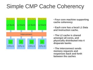
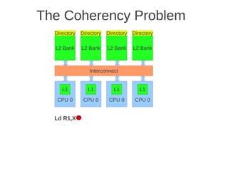
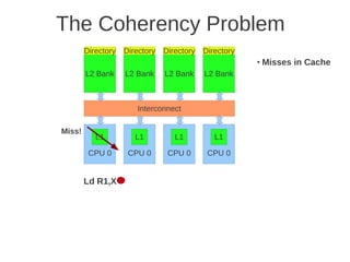
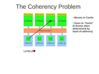
b) (Max 5 points) Outline the main architecture in SUN’s T1 (Niagara) multicore processor. Describe the
placement of L1 and L2 cache, as well as how the L1 caches are kept coherent.
Fig 4.24 at page 250 in the textbook, that shows 8 cores, each with its own L1-cache (described in the text), 4 x
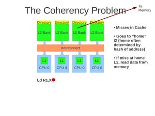
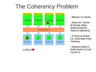
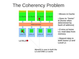
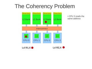
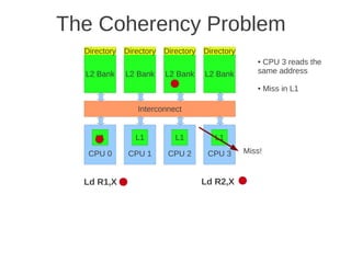
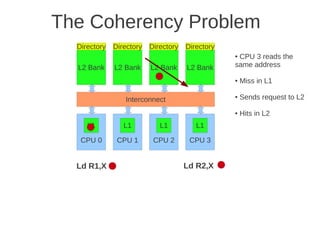
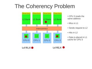
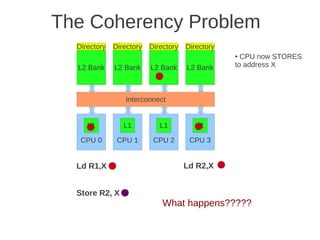
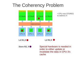
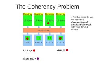
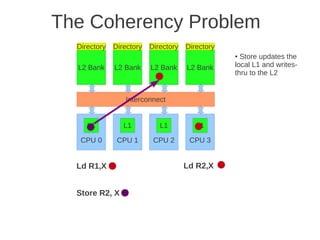
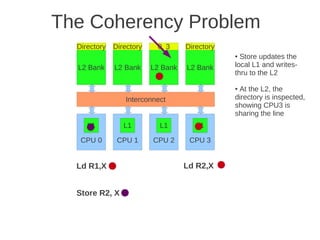
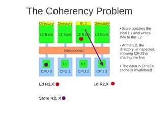
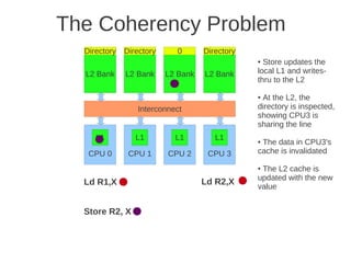
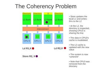
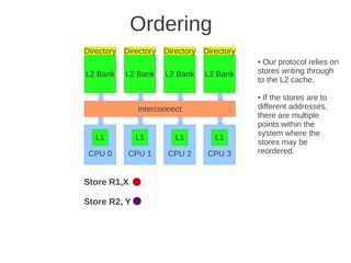
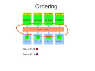
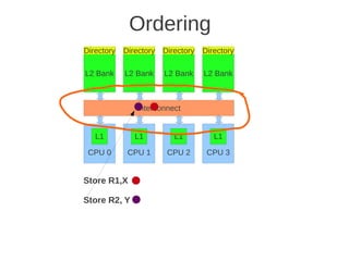
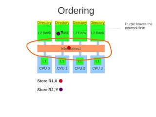
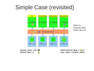
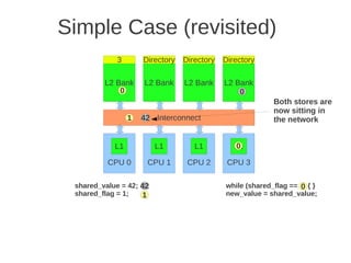
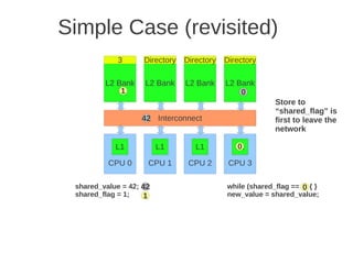
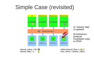
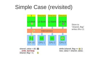
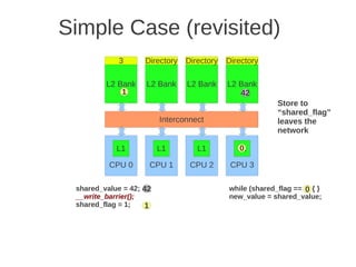
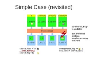
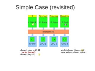
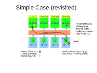
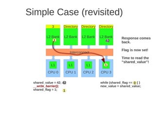
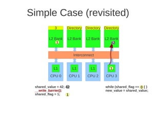
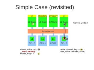
L2 cache banks, each having a channel to external memory, 1x FPU unit, crossbar as interconnection. Coherence](https://image.slidesharecdn.com/tdt4260-110828142109-phpapp02/85/tdt4260-350-320.jpg)

The course aims to provide a deep understanding of modern computer organization and architectures, with a focus on hardware and low-level software interactions, parallelism, and principles rather than details. It covers topics like instruction-level parallelism, memory hierarchies, multiprocessors, and interconnection networks. Evaluation is based on an obligatory exercise worth 20% and a final written exam worth 80%. The course infrastructure includes the Stallo compute cluster for simulating new multicore architectures.


![[ppt]](https://cdn.slidesharecdn.com/ss_thumbnails/ppt990-thumbnail.jpg?width=640&height=640&fit=bounds)


![[Harvard CS264] 02 - Parallel Thinking, Architecture, Theory & Patterns](https://cdn.slidesharecdn.com/ss_thumbnails/cs264201102-archtheorypatternshare-110206154047-phpapp02-thumbnail.jpg?width=640&height=640&fit=bounds)


![Unitplan eit[1]](https://cdn.slidesharecdn.com/ss_thumbnails/unitplaneit1-110920034359-phpapp01-thumbnail.jpg?width=640&height=640&fit=bounds)


