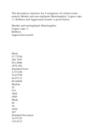
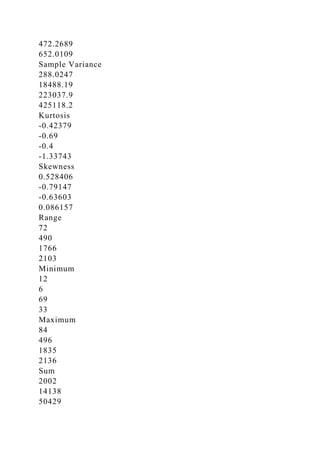
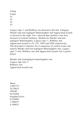
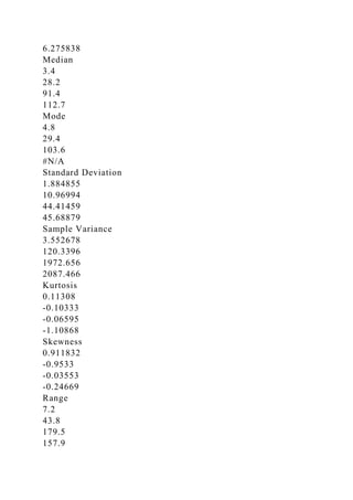
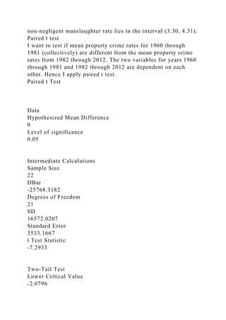
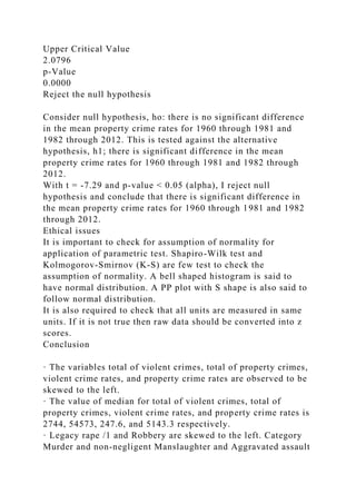
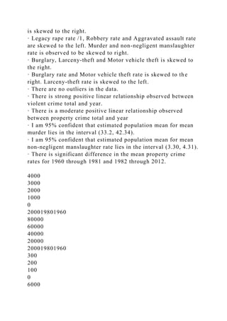
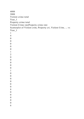
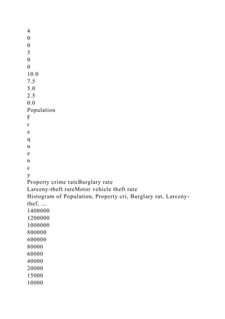
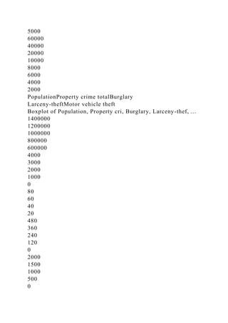
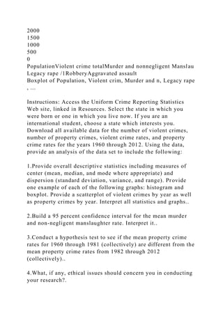
Table of Contents
Introduction 2
Descriptive statistics 3
Violent and property crimes 3
Categories of Violent and property crimes 5
Graphical Representation 9
Histogram 9
Boxplot 11
Scatterplot 12
Confidence interval 13
Murder 13
Non-negligent manslaughter rate 14
Paired t test 15
Ethical issues 17
Conclusion 18
Introduction
I consider data sets namely number of violent crimes, number of
property crimes, violent crime rates, and property crime rates
for the years 1960 through 2012 for my analysis. Violent crime
have has 4 categories Murder and non-negligent Manslaughter,
Legacy rape /1, Robbery and Aggravated assault. Property
crimes has 3 categories Burglary, Larceny-theft and Motor
vehicle theft.
Descriptive statisticsViolent and property crimes
The table of descriptive statistics for total of violent crimes,
total of property crimes, violent crime rates, and property crime
rates along with population is given below.
Population
Violent crime total
Property crime total
Violent Crime rate
Property crime rate
Mean
1027647.396
2332.321
51414.22642
213.0736
4940.675
Standard Error
30163.37005
152.2037
2356.550621
11.26415
179.483
Median
1062000
2744
54573
247.6
5143.3
Mode
1187000
#N/A
#N/A
231.9
#N/A
Standard Deviation
219592.6486
1108.06
17155.94748
82.00426
1306.656
Sample Variance
48220931312
1227797
294326533.9
6724.699
1707349
Kurtosis
-1.241236819
-0.76307
-0.34898103
0.141618
-0.73214
Skewness
-0.208033283
-0.78788
-0.684862884
-1.25813
-0.43517
Range
757318
3470
67533
277.7
4906.3
Minimum
632772
138
14405
21.8
2276.5
Maximum
1390090
3608
81938
299.5
7182.8
Sum
54465312
123613
2724954
11292.9
261855.8
Count
53
53
53
53
53
There are 53 observation for each year from 1960 to 2012. All
the variables total of violent crimes, total of property crimes,
violent crime rates, and property crime rates are observed to be
skewed to the left. For a skewed data, median is considered as
the best measure of central tendency. Median is the middle
observation in a series of data when arranged in ascending
order. The value of median for total of violent crimes, total of
property crimes, violent crime rates, and property crime rates is
2744, 54573, 247.6, and 5143.3 respectively.
Mean is defined as the sum of all observation divided by
total number of observations. The mean value for total of
violent crimes, total of property crimes, violent crime rates, and
property crime rates is 2332.321, 51414.22, 213.07 and 4940.67
respectively. The value of standard deviation and variance is a
measure of dispersion around mean. The value of standard
deviation for total of violent crimes, total of property crimes,
violent crime rates, and property crime rates is 1108.06,
17155.94, 82 and 1306.65. The low value of standard deviation
of Violent Crime rate and Property crime rate implies that its
mean is reliable. But high value of standard deviation of total of
violent crimes and total of property crimes implies that mean is
not reliable.
Categories of Violent and property crimes
The descriptive statistics for 4 categories of violent crime
namely Murder and non-negligent Manslaughter, Legacy rape
/1, Robbery and Aggravated assault is given below.
Murder and nonnegligent Manslaughter
Legacy rape /1
Robbery
Aggravated assault
Mean
37.77358
266.7547
951.4906
1076.302
Standard Error
2.331186
18.67709
64.87113
89.56058
Median
35
333
1065
1095
Mode
44
18
1030
387
Standard Deviation
16.97129
135.9713
472.2689
652.0109
Sample Variance
288.0247
18488.19
223037.9
425118.2
Kurtosis
-0.42379
-0.69
-0.4
-1.33743
Skewness
0.528406
-0.79147
-0.63603
0.086157
Range
72
490
1766
2103
Minimum
12
6
69
33
Maximum
84
496
1835
2136
Sum
2002
14138
50429
57044
Count
53
53
53
53
Legacy rape /1 and Robbery are skewed to the left. Category
Murder and non-negligent Manslaughter and Aggravated assault
is skewed to the right. For a skewed data median is the best
measure of central tendency. Median for Murder and non-
negligent Manslaughter, Legacy rape /1, Robbery and
Aggravated assault is 35, 333, 1065 and 1095 respectively.
The descriptive statistics for 4 categories of violent crime rate
namely Murder and non-negligent Manslaughter rate, Legacy
rape /1 rate, Robbery rate and Aggravated assault rate is given
below.
Murder and nonnegligent manslaughter rate
Legacy rape rate /1
Robbery rate
Aggravated assault rate
Mean
3.803774
24.29623
#NUM!
95.91698
Standard Error
0.258905
1.506837
6.100813
6.275838
Median
3.4
28.2
91.4
112.7
Mode
4.8
29.4
103.6
#N/A
Standard Deviation
1.884855
10.96994
44.41459
45.68879
Sample Variance
3.552678
120.3396
1972.656
2087.466
Kurtosis
0.11308
-0.10333
-0.06595
-1.10868
Skewness
0.911832
-0.9533
-0.03553
-0.24669
Range
7.2
43.8
179.5
157.9
Minimum
1.5
0.8
10.7
5.2
Maximum
8.7
44.6
190.2
163.1
Sum
201.6
1287.7
4719.8
5083.6
Count
53
53
53
53
Legacy rape rate /1, Robbery rate and Aggravated assault rate
are skewed to the left. Murder and non-negligent manslaughter
rate is observed to be skewed to right. Median for Murder and
non-negligent Manslaughter rate, Legacy rape /1 rate, Robbery
rate and Aggravated assault rate is 3.4, 28.2, 91.4 and 112.7
respectively.
The descriptive statistics for 3 categories of Property crime
namely Burglary, Larceny-theft and Motor vehicle theft is given
below.
Burglary
Larceny-theft
Motor vehicle theft
Mean
11550.71698
35022.71698
4840.792453
Standard Error
491.1478169
1817.827423
270.3117473
Median
11409
38329
4469
Mode
#N/A
#N/A
3635
Standard Deviation
3575.610079
13233.9834
1967.899225
Sample Variance
12784987.44
175138316.6
3872627.36
Kurtosis
-0.299426563
-0.645813313
0.43830898
Skewness
-0.344400434
-0.478107721
0.754527051
Range
14494
50538
8236
Minimum
3328
9369
1674
Maximum
17822
59907
9910
Sum
612188
1856204
256562
Count
53
53
53
Burglary, Larceny-theft and Motor vehicle theft is skewed to
the right. For a skewed data, median is the best measure of
central tendency. Median for Burglary, Larceny-theft and Motor
vehicle theft is11409, 38329 and 4469.
The descriptive statistics for Burglary rate, Larceny-theft rate
and Motor vehicle theft rate is given below.
Burglary rate
Larceny-theft rate
Motor vehicle theft rate
Mean
1152.815
3324.311
463.5264
Standard Error
54.71263
132.7419
19.0792
Median
1152.4
3544.3
430.1
Mode
#N/A
#N/A
#N/A
Standard Deviation
398.314
966.3753
138.8987
Sample Variance
158654
933881.2
19292.84
Kurtosis
-0.72562
-0.86604
-0.38551
Skewness
0.374369
-0.39523
0.553889
Range
1411.8
3566.3
557.6
Minimum
525.9
1480.6
241.2
Maximum
1937.7
5046.9
798.8
Sum
61099.2
176188.5
24566.9
Count
53
53
53
Burglary rate and Motor vehicle theft rate is skewed to the
right. Larceny-theft rate is skewed to the left. For a skewed
data, median is the best measure of central tendency. Median
for Burglary rate, Larceny-theft rate and Motor vehicle theft
rate is 1152.4, 3544.3 and 430.1 respectively.
Graphical Representation
Histogram
The histogram violent crime rates (as well as its categories) for
the years 1960 through 2012 is given below.
Legacy rape rate /1, Robbery rate and Aggravated assault rate
are skewed to the left. Murder and non-negligent manslaughter
rate is observed to be skewed to right. This implies there are
very few years with low Legacy rape rate /1, Robbery rate and
Aggravated assault rate. Also, there are very few years with
high Murder and non-negligent manslaughter rate.
The histogram property crime rates (as well as its categories)
for the years 1960 through 2012 is given below.
Burglary rate and Motor vehicle theft rate is skewed to the
right. Larceny-theft rate is skewed to the left. This implies there
are very few years with high Burglary rate and Motor vehicle
theft rate. Also, there are very few years with low Larceny-theft
rate.
Boxplot
The boxplot for total property crimes (as well as its categories)
for the years 1960 through 2012 is given below. I observe that
there are no outliers in the data.
The boxplot for total violent crimes (as well as its categories)
for the years 1960 through 2012 is given below. I observe that
there are no outliers in the data.
Scatterplot
The scatterplot for namely number of violent crimes, number of
property crimes, violent crime rates, and property crime rates
for the years 1960 through 2012 is given below.
There is strong positive linear relationship observed between
violent crime total and year as well as violent crime rate and
year. That with every year, the value of total violent crime
increases. With increase in every year, the value of violent
crime rate also increases.
There is a moderate positive linear relationship observed
between property crime total and year as well as property crime
rate and year. That with every year, the value of total property
crime increases. With increase in every year, the value of
property crime rate also increases.
Confidence interval
The 95% confidence interval for the mean murder and non-
negligent manslaughter rate is calculated with the help of
following formula.
Murder
The 95% confidence interval for the mean murder is (33.2,
42.34). Calculations are shown below.
Confidence Interval Estimate for the Mean
Data
Population Standard Deviation
16.971
Sample Mean
37.77358491
Sample Size
53
Confidence Level
95%
Intermediate Calculations
Standard Error of the Mean
2.3311
Z Value
-1.9600
Interval Half Width
4.5690
Confidence Interval
Interval Lower Limit
33.20
Interval Upper Limit
42.34
I am 95% confident that estimated population mean for mean
murder lies in the interval (33.2, 42.34).
Non-negligent manslaughter rate
The 95% confidence interval for the mean non-negligent
manslaughter rate is (3.30, 4.31). Calculations are shown below.
Confidence Interval Estimate for the Mean
Data
Population Standard Deviation
1.884
Sample Mean
3.803773585
Sample Size
53
Confidence Level
95%
Intermediate Calculations
Standard Error of the Mean
0.2588
Z Value
-1.9600
Interval Half Width
0.5072
Confidence Interval
Interval Lower Limit
3.30
Interval Upper Limit
4.31
I am 95% confident that estimated population mean for mean
non-negligent manslaughter rate lies in the interval (3.30, 4.31).
Paired t test
I want to test if mean property crime rates for 1960 through
1981 (collectively) are different from the mean property crime
rates from 1982 through 2012. The two variables for years 1960
through 1981 and 1982 through 2012 are dependent on each
other. Hence I apply paired t test.
Paired t Test
Data
Hypothesized Mean Difference
0
Level of significance
0.05
Intermediate Calculations
Sample Size
22
DBar
-25768.3182
Degrees of Freedom
21
SD
16572.0207
Standard Error
3533.1667
t Test Statistic
-7.2933
Two-Tail Test
Lower Critical Value
-2.0796
Upper Critical Value
2.0796
p-Value
0.0000
Reject the null hypothesis
Consider null hypothesis, ho: there is no significant difference
in the mean property crime rates for 1960 through 1981 and
1982 through 2012. This is tested against the alternative
hypothesis, h1; there is significant difference in the mean
property crime rates for 1960 through 1981 and 1982 through
2012.
With t = -7.29 and p-value < 0.05 (alpha), I reject null
hypothesis and conclude that there is significant difference in
the mean property crime rates for 1960 through 1981 and 1982
through 2012.
Ethical issues
It is important to check for assumption of normality for
application of parametric test. Shapiro-Wilk test and
Kolmogorov-Smirnov (K-S) are few test to check the
assumption of normality. A bell shaped histogram is said to
have normal distribution. A PP plot with S shape is also said to
follow normal distribution.
It is also required to check that all units are measured in same
units. If it is not true then raw data should be converted into z
scores.
Conclusion
· The variables total of violent crimes, total of property crimes,
violent crime rates, and property crime rates are observed to be
skewed to the left.
· The value of median for total of violent crimes, total of
property crimes, violent crime rates, and property crime rates is
2744, 54573, 247.6, and 5143.3 respectively.
· Legacy rape /1 and Robbery are skewed to the left. Category
Murder and non-negligent Manslaughter and Aggravated assault
is skewed to the right.
· Legacy rape rate /1, Robbery rate and Aggravated assault rate
are skewed to the left. Murder and non-negligent manslaughter
rate is observed to be skewed to right.
· Burglary, Larceny-theft and Motor vehicle theft is skewed to
the right.
· Burglary rate and Motor vehicle theft rate is skewed to the
right. Larceny-theft rate is skewed to the left.
· There are no outliers in the data.
· There is strong positive linear relationship observed between
violent crime total and year.
· There is a moderate positive linear relationship observed
between property crime total and year
· I am 95% confident that estimated population mean for mean
murder lies in the interval (33.2, 42.34).
· I am 95% confident that estimated population mean for mean
non-negligent manslaughter rate lies in the interval (3.30, 4.31).
· There is significant difference in the mean property crime
rates for 1960 through 1981 and 1982 through 2012.
4000
3000
2000
1000
0
200019801960
80000
60000
40000
20000
200019801960
300
200
100
0
6000
4000
2000
Violent crime total
Year_1
Property crime total
Violent Crime rateProperty crime rate
Scatterplot of Violent crim, Property cri, Violent Crim, ... vs
Year_1
1
4
0
0
0
0
0
1
2
0
0
0
0
0
1
0
0
0
0
0
0
8
0
0
0
0
0
6
0
0
0
0
0
12
9
6
3
0
3
0
0
2
4
0
1
8
0
1
2
0
6
0
20
15
10
5
0
8
.
0
6
.
4
4
.
8
3
.
2
1
.
6
10.0
7.5
5.0
2.5
0.0
4
0
3
0
2
0
1
00
20
15
10
5
0
2
0
0
1
6
0
1
2
0
8
0
4
0
16
12
8
4
0
1
6
0
1
2
0
8
0
4
00
12
9
6
3
0
Population
F
r
e
q
u
e
n
c
y
Violent Crime rateMurder and nonnegligent manslau
Legacy rape rate /1Robbery rateAggravated assault rate
Histogram of Population, Violent Crim, Murder and n, Legacy
rape , ...
1
4
0
0
0
0
0
1
2
0
0
0
0
0
1
0
0
0
0
0
0
8
0
0
0
0
0
6
0
0
0
0
0
12
9
6
3
0
7
0
0
0
6
0
0
0
5
0
0
0
4
0
0
0
3
0
0
0
8
6
4
2
0
1
8
0
0
1
6
0
0
1
4
0
0
1
2
0
0
1
0
0
0
8
0
0
6
0
0
8
6
4
2
0
5
0
0
0
4
5
0
0
4
0
0
0
3
5
0
0
3
0
0
0
2
5
0
0
2
0
0
0
1
5
0
0
12
9
6
3
0
8
0
0
7
0
0
6
0
0
5
0
0
4
0
0
3
0
0
10.0
7.5
5.0
2.5
0.0
Population
F
r
e
q
u
e
n
c
y
Property crime rateBurglary rate
Larceny-theft rateMotor vehicle theft rate
Histogram of Population, Property cri, Burglary rat, Larceny-
thef, ...
1400000
1200000
1000000
800000
600000
80000
60000
40000
20000
15000
10000
5000
60000
40000
20000
10000
8000
6000
4000
2000
PopulationProperty crime totalBurglary
Larceny-theftMotor vehicle theft
Boxplot of Population, Property cri, Burglary, Larceny-thef, ...
1400000
1200000
1000000
800000
600000
4000
3000
2000
1000
0
80
60
40
20
480
360
240
120
0
2000
1500
1000
500
0
2000
1500
1000
500
0
PopulationViolent crime totalMurder and nonnegligent Manslau
Legacy rape /1RobberyAggravated assault
Boxplot of Population, Violent crim, Murder and n, Legacy rape
, ...
Instructions: Access the Uniform Crime Reporting Statistics
Web site, linked in Resources. Select the state in which you
were born or one in which you live now. If you are an
international student, choose a state which interests you.
Download all available data for the number of violent crimes,
number of property crimes, violent crime rates, and property
crime rates for the years 1960 through 2012. Using the data,
provide an analysis of the data set to include the following:
1.Provide overall descriptive statistics including measures of
center (mean, median, and mode where appropriate) and
dispersion (standard deviation, variance, and range). Provide
one example of each of the following graphs: histogram and
boxplot. Provide a scatterplot of violent crimes by year as well
as property crimes by year. Interpret all statistics and graphs..
2.Build a 95 percent confidence interval for the mean murder
and non-negligent manslaughter rate. Interpret it..
3.Conduct a hypothesis test to see if the mean property crime
rates for 1960 through 1981 (collectively) are different from the
mean property crime rates from 1982 through 2012
(collectively)..
4.What, if any, ethical issues should concern you in conducting
your research?.
Complete your report in a Word document (submitted as a .docx
file), including relevant tables and graphics you need to support
your findings. Place your tables and graphics within the text and
be sure to clearly title them. Your tables and graphics must be
legible and suitable for inclusion in a management report.
Before you submit your assignment to your instructor for
grading, submit a final version of your paper to Turnitin.
Assignments must be submitted to the assignments area for
grading. Work e-mailed or otherwise presented cannot be
graded in accordance with Capella grading standards. Refer to
the scoring guide to ensure that you meet the grading criteria
for this assessment.
The link to Access the Uniform Crime Reporting Statistics Web
site
https://www.ucrdatatool.gov/Search/Crime/State/StatebyState.cf
m

Table of ContentsIntroduction2Descriptive statistics3Viole.docx

  • 1.
    Table of Contents Introduction2 Descriptive statistics 3 Violent and property crimes 3 Categories of Violent and property crimes 5 Graphical Representation 9 Histogram 9 Boxplot 11 Scatterplot 12 Confidence interval 13 Murder 13 Non-negligent manslaughter rate 14 Paired t test 15 Ethical issues 17 Conclusion 18 Introduction I consider data sets namely number of violent crimes, number of property crimes, violent crime rates, and property crime rates for the years 1960 through 2012 for my analysis. Violent crime have has 4 categories Murder and non-negligent Manslaughter, Legacy rape /1, Robbery and Aggravated assault. Property crimes has 3 categories Burglary, Larceny-theft and Motor vehicle theft. Descriptive statisticsViolent and property crimes The table of descriptive statistics for total of violent crimes, total of property crimes, violent crime rates, and property crime rates along with population is given below. Population Violent crime total Property crime total Violent Crime rate Property crime rate
  • 2.
  • 3.
  • 4.
    Sum 54465312 123613 2724954 11292.9 261855.8 Count 53 53 53 53 53 There are 53observation for each year from 1960 to 2012. All the variables total of violent crimes, total of property crimes, violent crime rates, and property crime rates are observed to be skewed to the left. For a skewed data, median is considered as the best measure of central tendency. Median is the middle observation in a series of data when arranged in ascending order. The value of median for total of violent crimes, total of property crimes, violent crime rates, and property crime rates is 2744, 54573, 247.6, and 5143.3 respectively. Mean is defined as the sum of all observation divided by total number of observations. The mean value for total of violent crimes, total of property crimes, violent crime rates, and property crime rates is 2332.321, 51414.22, 213.07 and 4940.67 respectively. The value of standard deviation and variance is a measure of dispersion around mean. The value of standard deviation for total of violent crimes, total of property crimes, violent crime rates, and property crime rates is 1108.06, 17155.94, 82 and 1306.65. The low value of standard deviation of Violent Crime rate and Property crime rate implies that its mean is reliable. But high value of standard deviation of total of violent crimes and total of property crimes implies that mean is not reliable. Categories of Violent and property crimes
  • 5.
    The descriptive statisticsfor 4 categories of violent crime namely Murder and non-negligent Manslaughter, Legacy rape /1, Robbery and Aggravated assault is given below. Murder and nonnegligent Manslaughter Legacy rape /1 Robbery Aggravated assault Mean 37.77358 266.7547 951.4906 1076.302 Standard Error 2.331186 18.67709 64.87113 89.56058 Median 35 333 1065 1095 Mode 44 18 1030 387 Standard Deviation 16.97129 135.9713
  • 6.
  • 7.
    57044 Count 53 53 53 53 Legacy rape /1and Robbery are skewed to the left. Category Murder and non-negligent Manslaughter and Aggravated assault is skewed to the right. For a skewed data median is the best measure of central tendency. Median for Murder and non- negligent Manslaughter, Legacy rape /1, Robbery and Aggravated assault is 35, 333, 1065 and 1095 respectively. The descriptive statistics for 4 categories of violent crime rate namely Murder and non-negligent Manslaughter rate, Legacy rape /1 rate, Robbery rate and Aggravated assault rate is given below. Murder and nonnegligent manslaughter rate Legacy rape rate /1 Robbery rate Aggravated assault rate Mean 3.803774 24.29623 #NUM! 95.91698 Standard Error 0.258905 1.506837 6.100813
  • 8.
  • 9.
    Minimum 1.5 0.8 10.7 5.2 Maximum 8.7 44.6 190.2 163.1 Sum 201.6 1287.7 4719.8 5083.6 Count 53 53 53 53 Legacy rape rate/1, Robbery rate and Aggravated assault rate are skewed to the left. Murder and non-negligent manslaughter rate is observed to be skewed to right. Median for Murder and non-negligent Manslaughter rate, Legacy rape /1 rate, Robbery rate and Aggravated assault rate is 3.4, 28.2, 91.4 and 112.7 respectively. The descriptive statistics for 3 categories of Property crime namely Burglary, Larceny-theft and Motor vehicle theft is given below. Burglary Larceny-theft Motor vehicle theft
  • 10.
    Mean 11550.71698 35022.71698 4840.792453 Standard Error 491.1478169 1817.827423 270.3117473 Median 11409 38329 4469 Mode #N/A #N/A 3635 Standard Deviation 3575.610079 13233.9834 1967.899225 SampleVariance 12784987.44 175138316.6 3872627.36 Kurtosis -0.299426563 -0.645813313 0.43830898 Skewness -0.344400434 -0.478107721 0.754527051 Range 14494
  • 11.
    50538 8236 Minimum 3328 9369 1674 Maximum 17822 59907 9910 Sum 612188 1856204 256562 Count 53 53 53 Burglary, Larceny-theft andMotor vehicle theft is skewed to the right. For a skewed data, median is the best measure of central tendency. Median for Burglary, Larceny-theft and Motor vehicle theft is11409, 38329 and 4469. The descriptive statistics for Burglary rate, Larceny-theft rate and Motor vehicle theft rate is given below. Burglary rate Larceny-theft rate Motor vehicle theft rate Mean 1152.815 3324.311
  • 12.
    463.5264 Standard Error 54.71263 132.7419 19.0792 Median 1152.4 3544.3 430.1 Mode #N/A #N/A #N/A Standard Deviation 398.314 966.3753 138.8987 SampleVariance 158654 933881.2 19292.84 Kurtosis -0.72562 -0.86604 -0.38551 Skewness 0.374369 -0.39523 0.553889 Range 1411.8 3566.3 557.6 Minimum 525.9 1480.6
  • 13.
    241.2 Maximum 1937.7 5046.9 798.8 Sum 61099.2 176188.5 24566.9 Count 53 53 53 Burglary rate andMotor vehicle theft rate is skewed to the right. Larceny-theft rate is skewed to the left. For a skewed data, median is the best measure of central tendency. Median for Burglary rate, Larceny-theft rate and Motor vehicle theft rate is 1152.4, 3544.3 and 430.1 respectively. Graphical Representation Histogram The histogram violent crime rates (as well as its categories) for the years 1960 through 2012 is given below. Legacy rape rate /1, Robbery rate and Aggravated assault rate are skewed to the left. Murder and non-negligent manslaughter rate is observed to be skewed to right. This implies there are very few years with low Legacy rape rate /1, Robbery rate and Aggravated assault rate. Also, there are very few years with high Murder and non-negligent manslaughter rate. The histogram property crime rates (as well as its categories) for the years 1960 through 2012 is given below. Burglary rate and Motor vehicle theft rate is skewed to the
  • 14.
    right. Larceny-theft rateis skewed to the left. This implies there are very few years with high Burglary rate and Motor vehicle theft rate. Also, there are very few years with low Larceny-theft rate. Boxplot The boxplot for total property crimes (as well as its categories) for the years 1960 through 2012 is given below. I observe that there are no outliers in the data. The boxplot for total violent crimes (as well as its categories) for the years 1960 through 2012 is given below. I observe that there are no outliers in the data. Scatterplot The scatterplot for namely number of violent crimes, number of property crimes, violent crime rates, and property crime rates for the years 1960 through 2012 is given below. There is strong positive linear relationship observed between violent crime total and year as well as violent crime rate and year. That with every year, the value of total violent crime increases. With increase in every year, the value of violent crime rate also increases. There is a moderate positive linear relationship observed between property crime total and year as well as property crime rate and year. That with every year, the value of total property crime increases. With increase in every year, the value of property crime rate also increases. Confidence interval The 95% confidence interval for the mean murder and non- negligent manslaughter rate is calculated with the help of
  • 15.
    following formula. Murder The 95%confidence interval for the mean murder is (33.2, 42.34). Calculations are shown below. Confidence Interval Estimate for the Mean Data Population Standard Deviation 16.971 Sample Mean 37.77358491 Sample Size 53 Confidence Level 95% Intermediate Calculations Standard Error of the Mean 2.3311 Z Value -1.9600 Interval Half Width 4.5690 Confidence Interval Interval Lower Limit 33.20 Interval Upper Limit 42.34 I am 95% confident that estimated population mean for mean
  • 16.
    murder lies inthe interval (33.2, 42.34). Non-negligent manslaughter rate The 95% confidence interval for the mean non-negligent manslaughter rate is (3.30, 4.31). Calculations are shown below. Confidence Interval Estimate for the Mean Data Population Standard Deviation 1.884 Sample Mean 3.803773585 Sample Size 53 Confidence Level 95% Intermediate Calculations Standard Error of the Mean 0.2588 Z Value -1.9600 Interval Half Width 0.5072 Confidence Interval Interval Lower Limit 3.30 Interval Upper Limit 4.31 I am 95% confident that estimated population mean for mean
  • 17.
    non-negligent manslaughter ratelies in the interval (3.30, 4.31). Paired t test I want to test if mean property crime rates for 1960 through 1981 (collectively) are different from the mean property crime rates from 1982 through 2012. The two variables for years 1960 through 1981 and 1982 through 2012 are dependent on each other. Hence I apply paired t test. Paired t Test Data Hypothesized Mean Difference 0 Level of significance 0.05 Intermediate Calculations Sample Size 22 DBar -25768.3182 Degrees of Freedom 21 SD 16572.0207 Standard Error 3533.1667 t Test Statistic -7.2933 Two-Tail Test Lower Critical Value -2.0796
  • 18.
    Upper Critical Value 2.0796 p-Value 0.0000 Rejectthe null hypothesis Consider null hypothesis, ho: there is no significant difference in the mean property crime rates for 1960 through 1981 and 1982 through 2012. This is tested against the alternative hypothesis, h1; there is significant difference in the mean property crime rates for 1960 through 1981 and 1982 through 2012. With t = -7.29 and p-value < 0.05 (alpha), I reject null hypothesis and conclude that there is significant difference in the mean property crime rates for 1960 through 1981 and 1982 through 2012. Ethical issues It is important to check for assumption of normality for application of parametric test. Shapiro-Wilk test and Kolmogorov-Smirnov (K-S) are few test to check the assumption of normality. A bell shaped histogram is said to have normal distribution. A PP plot with S shape is also said to follow normal distribution. It is also required to check that all units are measured in same units. If it is not true then raw data should be converted into z scores. Conclusion · The variables total of violent crimes, total of property crimes, violent crime rates, and property crime rates are observed to be skewed to the left. · The value of median for total of violent crimes, total of property crimes, violent crime rates, and property crime rates is 2744, 54573, 247.6, and 5143.3 respectively. · Legacy rape /1 and Robbery are skewed to the left. Category Murder and non-negligent Manslaughter and Aggravated assault
  • 19.
    is skewed tothe right. · Legacy rape rate /1, Robbery rate and Aggravated assault rate are skewed to the left. Murder and non-negligent manslaughter rate is observed to be skewed to right. · Burglary, Larceny-theft and Motor vehicle theft is skewed to the right. · Burglary rate and Motor vehicle theft rate is skewed to the right. Larceny-theft rate is skewed to the left. · There are no outliers in the data. · There is strong positive linear relationship observed between violent crime total and year. · There is a moderate positive linear relationship observed between property crime total and year · I am 95% confident that estimated population mean for mean murder lies in the interval (33.2, 42.34). · I am 95% confident that estimated population mean for mean non-negligent manslaughter rate lies in the interval (3.30, 4.31). · There is significant difference in the mean property crime rates for 1960 through 1981 and 1982 through 2012. 4000 3000 2000 1000 0 200019801960 80000 60000 40000 20000 200019801960 300 200 100 0 6000
  • 20.
    4000 2000 Violent crime total Year_1 Propertycrime total Violent Crime rateProperty crime rate Scatterplot of Violent crim, Property cri, Violent Crim, ... vs Year_1 1 4 0 0 0 0 0 1 2 0 0 0 0 0 1 0 0 0 0 0 0 8 0 0 0 0 0 6
  • 21.
  • 22.
  • 23.
    0 4 0 16 12 8 4 0 1 6 0 1 2 0 8 0 4 00 12 9 6 3 0 Population F r e q u e n c y Violent Crime rateMurderand nonnegligent manslau Legacy rape rate /1Robbery rateAggravated assault rate Histogram of Population, Violent Crim, Murder and n, Legacy
  • 24.
  • 25.
  • 26.
  • 27.
  • 28.
    4 0 0 3 0 0 10.0 7.5 5.0 2.5 0.0 Population F r e q u e n c y Property crime rateBurglaryrate Larceny-theft rateMotor vehicle theft rate Histogram of Population, Property cri, Burglary rat, Larceny- thef, ... 1400000 1200000 1000000 800000 600000 80000 60000 40000 20000 15000 10000
  • 29.
    5000 60000 40000 20000 10000 8000 6000 4000 2000 PopulationProperty crime totalBurglary Larceny-theftMotorvehicle theft Boxplot of Population, Property cri, Burglary, Larceny-thef, ... 1400000 1200000 1000000 800000 600000 4000 3000 2000 1000 0 80 60 40 20 480 360 240 120 0 2000 1500 1000 500 0
  • 30.
    2000 1500 1000 500 0 PopulationViolent crime totalMurderand nonnegligent Manslau Legacy rape /1RobberyAggravated assault Boxplot of Population, Violent crim, Murder and n, Legacy rape , ... Instructions: Access the Uniform Crime Reporting Statistics Web site, linked in Resources. Select the state in which you were born or one in which you live now. If you are an international student, choose a state which interests you. Download all available data for the number of violent crimes, number of property crimes, violent crime rates, and property crime rates for the years 1960 through 2012. Using the data, provide an analysis of the data set to include the following: 1.Provide overall descriptive statistics including measures of center (mean, median, and mode where appropriate) and dispersion (standard deviation, variance, and range). Provide one example of each of the following graphs: histogram and boxplot. Provide a scatterplot of violent crimes by year as well as property crimes by year. Interpret all statistics and graphs.. 2.Build a 95 percent confidence interval for the mean murder and non-negligent manslaughter rate. Interpret it.. 3.Conduct a hypothesis test to see if the mean property crime rates for 1960 through 1981 (collectively) are different from the mean property crime rates from 1982 through 2012 (collectively).. 4.What, if any, ethical issues should concern you in conducting your research?.
  • 31.
    Complete your reportin a Word document (submitted as a .docx file), including relevant tables and graphics you need to support your findings. Place your tables and graphics within the text and be sure to clearly title them. Your tables and graphics must be legible and suitable for inclusion in a management report. Before you submit your assignment to your instructor for grading, submit a final version of your paper to Turnitin. Assignments must be submitted to the assignments area for grading. Work e-mailed or otherwise presented cannot be graded in accordance with Capella grading standards. Refer to the scoring guide to ensure that you meet the grading criteria for this assessment. The link to Access the Uniform Crime Reporting Statistics Web site https://www.ucrdatatool.gov/Search/Crime/State/StatebyState.cf m