Structural Equation Modeling concepts and applications.ppt
1.
v2.3 Petri Nokelainen,University of Tampere, Finland
Structural Equation Modeling
Petri Nokelainen
School of Education
University of Tampere, Finland
petri.nokelainen@uta.fi
http://www.uta.fi/~petri.nokelainen
2.
Petri Nokelainen, Universityof Tampere, Finland 2 / 145
Contents
Introduction
Path Analysis
Basic Concepts of Factor Analysis
Model Constructing
Model hypotheses
Model specification
Model identification
Model estimation
An Example of SEM: Commitment to Work and
Organization
Conclusions
References
v2.3
3.
Petri Nokelainen, Universityof Tampere, Finland 3 / 145
Introduction
Development of Western science is based on two
great achievements: the invention of the formal
logical system (in Euclidean geometry) by the
Greek philosophers, and the possibility to find out
causal relationships by systematic experiment
(during the Renaissance).
Albert Einstein
(in Pearl, 2000)
v2.3
4.
Petri Nokelainen, Universityof Tampere, Finland 4 / 145
Introduction
Structural equation modeling (SEM), as a
concept, is a combination of statistical
techniques such as exploratory factor
analysis and multiple regression.
The purpose of SEM is to examine a set of
relationships between one or more
Independent Variables (IV) and one or
more Dependent Variables (DV).
v2.3
5.
Petri Nokelainen, Universityof Tampere, Finland 5 / 145
Introduction
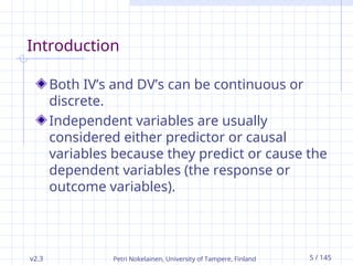
Both IV’s and DV’s can be continuous or
discrete.
Independent variables are usually
considered either predictor or causal
variables because they predict or cause the
dependent variables (the response or
outcome variables).
v2.3
6.
Petri Nokelainen, Universityof Tampere, Finland 6 / 145
Introduction
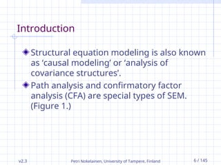
Structural equation modeling is also known
as ‘causal modeling’ or ‘analysis of
covariance structures’.
Path analysis and confirmatory factor
analysis (CFA) are special types of SEM.
(Figure 1.)
v2.3
7.
Petri Nokelainen, Universityof Tampere, Finland 7 / 145
Introduction
Genetics S. Wright (1921): “Prior knowledge of
the causal relations is assumed as prerequisite
… [in linear structural modeling]”.
y = x +
“In an ideal experiment where we control X to x
and any other set Z of variables (not containing
X or Y) to z, the value of Y is given by x + ,
where is not a function of the settings x and z.”
(Pearl, 2000)
v2.3
8.
Petri Nokelainen, Universityof Tampere, Finland 8 / 145
Introduction
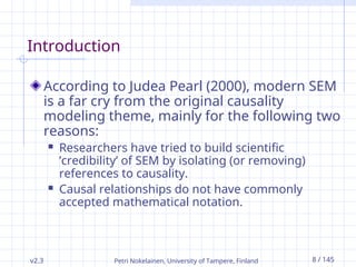
According to Judea Pearl (2000), modern SEM
is a far cry from the original causality
modeling theme, mainly for the following two
reasons:
Researchers have tried to build scientific
’credibility’ of SEM by isolating (or removing)
references to causality.
Causal relationships do not have commonly
accepted mathematical notation.
v2.3
9.
v2.3 Petri Nokelainen,University of Tampere, Finland 9 / 145
Introduction
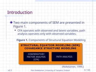
Figure 1. Components of Structural Equation Modeling
(Nokelainen, 1999.)
Two main components of SEM are presented in
Figure 1.
CFA operates with observed and latent variables, path
analysis operates only with observed variables.
10.
v2.3 Petri Nokelainen,University of Tampere, Finland 10 / 145
Contents
Introduction
Path Analysis
Basic Concepts of Factor Analysis
Model Constructing
Model hypotheses
Model specification
Model identification
Model estimation
An Example of SEM: Commitment to Work and
Organization
Conclusions
References
11.
v2.3 Petri Nokelainen,University of Tampere, Finland 11 / 145
Path Analysis
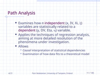
Examines how n independent (x, IV, Xi, )
variables are statistically related to a
dependent (y, DV, Eta, ) variable.
Applies the techniques of regression analysis,
aiming at more detailed resolution of the
phenomena under investigation.
Allows
Causal interpretation of statistical dependencies
Examination of how data fits to a theoretical model
12.
v2.3 Petri Nokelainen,University of Tampere, Finland 12 / 145
Path Analysis
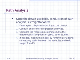
Once the data is available, conduction of path
analysis is straightforward:
1. Draw a path diagram according to the theory.
2. Conduct one or more regression analyses.
3. Compare the regression estimates (B) to the
theoretical assumptions or (Beta) other studies.
4. If needed, modify the model by removing or adding
connecting paths between the variables and redo
stages 2 and 3.
13.
v2.3 Petri Nokelainen,University of Tampere, Finland 13 / 145
Path Analysis
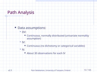
Data assumptions:
DV:
Continuous, normally distributed (univariate normality
assumption)
IV:
Continuous (no dichotomy or categorical variables)
N:
About 30 observations for each IV
14.
v2.3 Petri Nokelainen,University of Tampere, Finland 14 / 145
Path Analysis
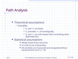
Theoretical assumptions
Causality:
X1 and Y1 correlate.
X1 precedes Y1 chronologically.
X1 and Y1 are still related after controlling other
dependencies.
Statistical assumptions
Model needs to be recursive.
It is OK to use ordinal data.
All variables are measured (and analyzed) without
measurement error ( = 0).
15.
v2.3 Petri Nokelainen,University of Tampere, Finland 15 / 145
Path Analysis
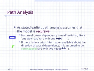
As stated earlier, path analysis assumes that
the model is recursive.
Nature of causal dependency is unidirectional, like a
’one way road’ (arc with one head ).
If there is no a priori information available about the
direction of causal dependency, it is assumed to be
correlational (arc with two heads ).
r
16.
v2.3 Petri Nokelainen,University of Tampere, Finland 16 / 145
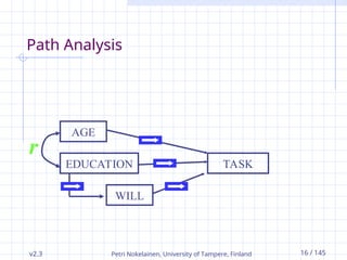
Path Analysis
r
AGE
EDUCATION
WILL
TASK
17.
v2.3 Petri Nokelainen,University of Tampere, Finland 17 / 145
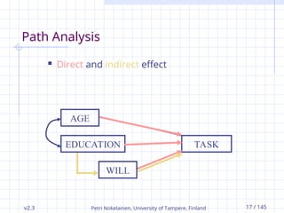
Path Analysis
Direct and indirect effect
AGE
EDUCATION
WILL
TASK
18.
v2.3 Petri Nokelainen,University of Tampere, Finland 18 / 145
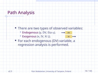
Path Analysis
There are two types of observed variables:
Endogenous (y, DV, Eta ).
Exogenous (x, IV, Xi ).
For each endogenous (DV) variable, a
regression analysis is performed.
DV
IV
19.
v2.3 Petri Nokelainen,University of Tampere, Finland 19 / 145
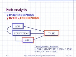
Path Analysis
AGE
EDUCATION
WILL
TASK
x IV Xi EXOGENIOUS
y DV Eta ENDOGENIOUS
Two regression analyses:
1) AGE + EDUCATION + WILL -> TASK
2) EDUCATION –> WILL
20.
v2.3 Petri Nokelainen,University of Tampere, Finland 20 / 145
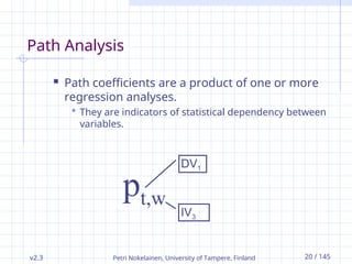
Path Analysis
Path coefficients are a product of one or more
regression analyses.
They are indicators of statistical dependency between
variables.
pt,w
DV1
IV3
21.
v2.3 Petri Nokelainen,University of Tampere, Finland 21 / 145
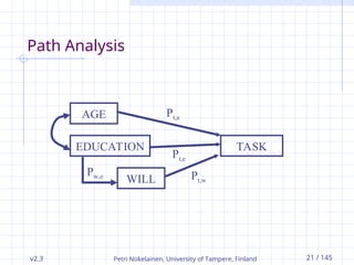
Path Analysis
AGE
EDUCATION
WILL
TASK
Pt,w
Pt,e
Pt,a
Pw,e
22.
v2.3 Petri Nokelainen,University of Tampere, Finland 22 / 145
Path Analysis
Path coefficients are standardized (´Beta´) or
unstandardized (´B´ or (´´) regression
coefficients.
Strength of inter-variable dependencies are
comparable to other studies when standardized
values (z, where M = 0 and SD = 1) are used.
Unstandardized values allow the original
measurement scale examination of inter-variable
dependencies.
1
)
( 2
N
x
x
SD
SD
x
x
z
)
(
23.
v2.3 Petri Nokelainen,University of Tampere, Finland 23 / 145
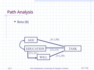
Path Analysis
AGE
EDUCATION
WILL
TASK
,31 (,39)
,12 (,13)
,41 (,50)
,23 (,31)
Beta (B)
24.
v2.3 Petri Nokelainen,University of Tampere, Finland 24 / 145
Path Analysis
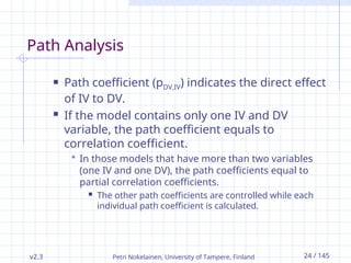
Path coefficient (pDV,IV) indicates the direct effect
of IV to DV.
If the model contains only one IV and DV
variable, the path coefficient equals to
correlation coefficient.
In those models that have more than two variables
(one IV and one DV), the path coefficients equal to
partial correlation coefficients.
The other path coefficients are controlled while each
individual path coefficient is calculated.
25.
v2.3 Petri Nokelainen,University of Tampere, Finland 25 / 145
Path Analysis
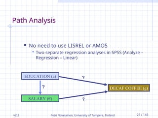
No need to use LISREL or AMOS
Two separate regression analyses in SPSS (Analyze –
Regression – Linear)
?
EDUCATION (a)
SALARY (€)
DECAF COFFEE (g)
?
?
26.
v2.3 Petri Nokelainen,University of Tampere, Finland 26 / 145
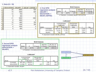
1. Data (N = 10)
2. First SPSS
regression analysis
(SALARY +
EDUCATION ->
DECAF_COFFEE)
3. Second SPSS
regression analysis
(EDUCATION ->
SALARY)
27.
v2.3 Petri Nokelainen,University of Tampere, Finland 27 / 145
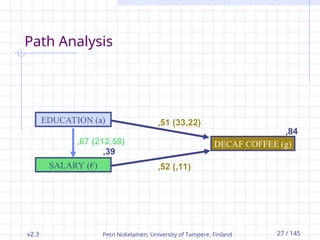
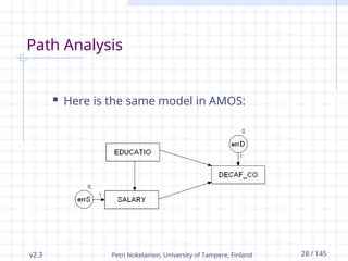
Path Analysis
,51 (33,22)
EDUCATION (a)
SALARY (€)
DECAF COFFEE (g)
,52 (,11)
,67 (212,58)
,84
,39
28.
v2.3 Petri Nokelainen,University of Tampere, Finland 28 / 145
Path Analysis
Here is the same model in AMOS:
29.
v2.3 Petri Nokelainen,University of Tampere, Finland 29 / 145
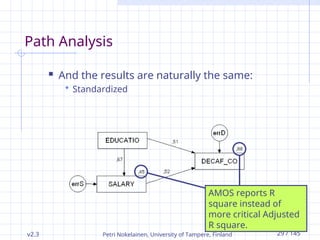
Path Analysis
And the results are naturally the same:
Standardized
AMOS reports R
square instead of
more critical Adjusted
R square.
30.
v2.3 Petri Nokelainen,University of Tampere, Finland 30 / 145
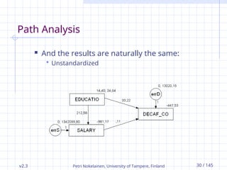
Path Analysis
And the results are naturally the same:
Unstandardized
31.
v2.3 Petri Nokelainen,University of Tampere, Finland 31 / 145
Contents
Introduction
Path Analysis
Basic Concepts of Factor Analysis
Model Constructing
Model hypotheses
Model specification
Model identification
Model estimation
An Example of SEM: Commitment to Work and
Organization
Conclusions
References
32.
v2.3 Petri Nokelainen,University of Tampere, Finland 32 / 145
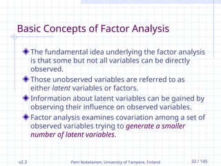
Basic Concepts of Factor Analysis
The fundamental idea underlying the factor analysis
is that some but not all variables can be directly
observed.
Those unobserved variables are referred to as
either latent variables or factors.
Information about latent variables can be gained by
observing their influence on observed variables.
Factor analysis examines covariation among a set of
observed variables trying to generate a smaller
number of latent variables.
33.
v2.3 Petri Nokelainen,University of Tampere, Finland 33 / 145
Basic Concepts of Factor Analysis
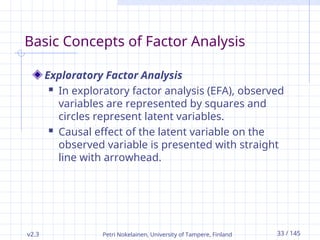
Exploratory Factor Analysis
In exploratory factor analysis (EFA), observed
variables are represented by squares and
circles represent latent variables.
Causal effect of the latent variable on the
observed variable is presented with straight
line with arrowhead.
34.
v2.3 Petri Nokelainen,University of Tampere, Finland 34 / 145
Basic Concepts of Factor Analysis
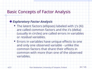
Exploratory Factor Analysis
The latent factors (ellipses) labeled with ’s (Xi)
are called common factors and the ’s (delta)
(usually in circles) are called errors in variables
or residual variables.
Errors in variables have unique effects to one
and only one observed variable - unlike the
common factors that share their effects in
common with more than one of the observed
variables.
35.
v2.3 Petri Nokelainen,University of Tampere, Finland 35 / 145
Basic Concepts of Factor Analysis
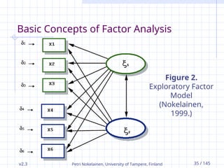
Figure 2.
Exploratory Factor
Model
(Nokelainen,
1999.)
36.
v2.3 Petri Nokelainen,University of Tampere, Finland 36 / 145
Basic Concepts of Factor Analysis
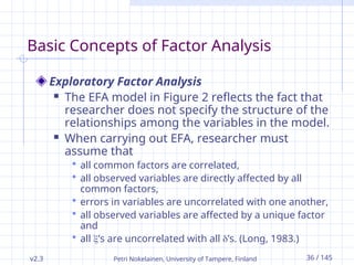
Exploratory Factor Analysis
The EFA model in Figure 2 reflects the fact that
researcher does not specify the structure of the
relationships among the variables in the model.
When carrying out EFA, researcher must
assume that
all common factors are correlated,
all observed variables are directly affected by all
common factors,
errors in variables are uncorrelated with one another,
all observed variables are affected by a unique factor
and
all ’s are uncorrelated with all ’s. (Long, 1983.)
37.
v2.3 Petri Nokelainen,University of Tampere, Finland 37 / 145
Basic Concepts of Factor Analysis
Confirmatory Factor Analysis
One of the biggest problems in EFA is its inability to
incorporate substantively meaningful constraints.
That is due to fact that algebraic mathematical solution
to solve estimates is not trivial, instead one has to seek
for other solutions.
That problem was partly solved by the development of
the confirmatory factor model, which was based on an
iterative algorithm (Jöreskog, 1969).
38.
v2.3 Petri Nokelainen,University of Tampere, Finland 38 / 145
Basic Concepts of Factor Analysis
Confirmatory Factor Analysis
In confirmatory factor analysis (CFA), which is a
special case of SEM, the correlations between
the factors are an explicit part of the analysis
because they are collected in a matrix of factor
correlations.
With CFA, researcher is able to decide a priori
whether the factors would correlate or not.
(Tacq, 1997.)
39.
v2.3 Petri Nokelainen,University of Tampere, Finland 39 / 145
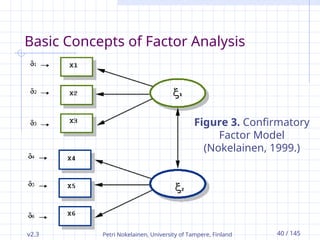
Basic Concepts of Factor Analysis
Confirmatory Factor Analysis
Moreover, researcher is able to impose
substantively motivated constraints,
which common factor pairs that are correlated,
which observed variables are affected by which
common factors,
which observed variables are affected by a unique
factor and
which pairs of unique factors are correlated.
(Long, 1983.)
40.
v2.3 Petri Nokelainen,University of Tampere, Finland 40 / 145
Basic Concepts of Factor Analysis
Figure 3. Confirmatory
Factor Model
(Nokelainen, 1999.)
41.
v2.3 Petri Nokelainen,University of Tampere, Finland 41 / 145
Contents
Introduction
Path Analysis
Basic Concepts of Factor Analysis
Model Constructing
Model hypotheses
Model specification
Model identification
Model estimation
An Example of SEM: Commitment to Work and
Organization
Conclusions
References
42.
v2.3 Petri Nokelainen,University of Tampere, Finland 42 / 145
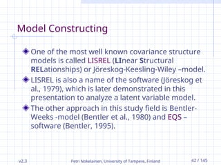
Model Constructing
One of the most well known covariance structure
models is called LISREL (LInear Structural
RELationships) or Jöreskog-Keesling-Wiley –model.
LISREL is also a name of the software (Jöreskog et
al., 1979), which is later demonstrated in this
presentation to analyze a latent variable model.
The other approach in this study field is Bentler-
Weeks -model (Bentler et al., 1980) and EQS –
software (Bentler, 1995).
43.
v2.3 Petri Nokelainen,University of Tampere, Finland 43 / 145
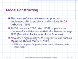
Model Constructing
The latest software release attempting to
implement SEM is graphical and intuitive AMOS
(Arbuckle, 1997).
AMOS has since 2000 taken LISREL’s place as a
module of a well-known statistical software package
SPSS (Statistical Package for Social Sciences).
Also other high quality SEM programs exist, such as
Mplus (Muthén & Muthén, 2000).
MPlus is targeted for professional users, it has only text
input mode.
44.
v2.3 Petri Nokelainen,University of Tampere, Finland 44 / 145
Model Constructing
In this presentation, I will use both the LISREL 8 –
software and AMOS 5 for SEM analysis and
PRELIS 2 –software (Jöreskog et al., 1985) for
preliminary data analysis.
All the previously mentioned approaches to SEM
use the same pattern for constructing the model:
1. model hypotheses,
2. model specification,
3. model identification and
4. model estimation.
45.
v2.3 Petri Nokelainen,University of Tampere, Finland 45 / 145
1. Model Hypotheses
Next, we will perform a CFA model
constructing process for a part of a
“Commitment to Work and Organization”
model.
This is quite technical approach but
unavoidable in order to understand the
underlying concepts and a way of
statistical thinking.
46.
v2.3 Petri Nokelainen,University of Tampere, Finland 46 / 145
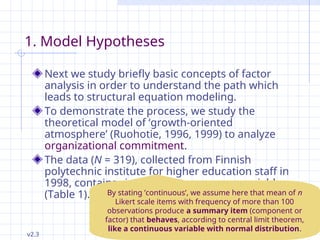
1. Model Hypotheses
Next we study briefly basic concepts of factor
analysis in order to understand the path which
leads to structural equation modeling.
To demonstrate the process, we study the
theoretical model of ‘growth-oriented
atmosphere’ (Ruohotie, 1996, 1999) to analyze
organizational commitment.
The data (N = 319), collected from Finnish
polytechnic institute for higher education staff in
1998, contains six continuous summary variables
(Table 1). By stating ’continuous’, we assume here that mean of n
Likert scale items with frequency of more than 100
observations produce a summary item (component or
factor) that behaves, according to central limit theorem,
like a continuous variable with normal distribution.
47.
v2.3 Petri Nokelainen,University of Tampere, Finland 47 / 145
F G
U R
N O
C U
T P
I
O
N
A
L
S M
U A
P N
P A
O G
R E
T M
I E
V N
E T
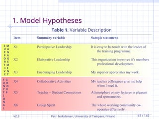
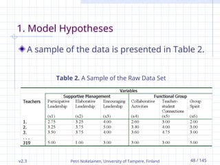
1. Model Hypotheses
Item Summary variable Sample statement
X1 Participative Leadership It is easy to be touch with the leader of
the training programme.
X2 Elaborative Leadership This organization improves it’s members
professional development.
X3 Encouraging Leadership My superior appreciates my work.
X4 Collaborative Activities My teacher colleagues give me help
when I need it.
X5 Teacher – Student Connections Athmosphere on my lectures is pleasant
and spontaneous.
X6 Group Spirit The whole working community co-
operates effectively.
Table 1. Variable Description
48.
v2.3 Petri Nokelainen,University of Tampere, Finland 48 / 145
1. Model Hypotheses
A sample of the data is presented in Table 2.
Table 2. A Sample of the Raw Data Set
49.
v2.3 Petri Nokelainen,University of Tampere, Finland 49 / 145
1. Model Hypotheses
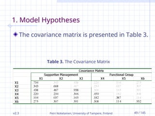
The covariance matrix is presented in Table 3.
Table 3. The Covariance Matrix
50.
v2.3 Petri Nokelainen,University of Tampere, Finland 50 / 145
1. Model Hypotheses
What is covariance matrix?
Scatter, covariance, and correlation matrix form the basis of a multivariate method.
The correlation and the covariance matrix are also often used for a first inspection of relationships among the variables of a multivariate data set.
All of these matrices are calculated using the matrix multiplication (A · B).
The only difference between them is how the data is scaled before the matrix multiplication is executed:
scatter: no scaling
covariance: mean of each variable is subtracted before multiplication
correlation: each variable is standardized (mean subtracted, then divided by standard deviation)
51.
v2.3 Petri Nokelainen,University of Tampere, Finland 51 / 145
1. Model Hypotheses
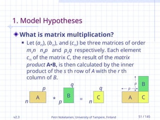
What is matrix multiplication?
Let (ars), (brs), and (crs) be three matrices of order
mxn nxp and pxq respectively. Each element
crs of the matrix C, the result of the matrix
product A•B, is then calculated by the inner
product of the s th row of A with the r th
column of B.
A B
*
n
p
p
q
= n
q
C C
A
B
p
p
52.
v2.3 Petri Nokelainen,University of Tampere, Finland 52 / 145
1. Model Hypotheses
The basic components of the confirmatory
factor model are illustrated in Figure 4.
Hypothesized model is sometimes called a
structural model.
53.
v2.3 Petri Nokelainen,University of Tampere, Finland 53 / 145
1. Model Hypotheses
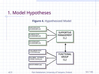
Figure 4. Hypothesized Model
54.
v2.3 Petri Nokelainen,University of Tampere, Finland 54 / 145
1. Model Hypotheses
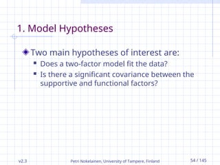
Two main hypotheses of interest are:
Does a two-factor model fit the data?
Is there a significant covariance between the
supportive and functional factors?
55.
v2.3 Petri Nokelainen,University of Tampere, Finland 55 / 145
2. Model Specification
Because of confirmatory nature of SEM, we
continue our model constructing with the
model specification to the stage, which is
referred as measurement model (Figure 5).
56.
v2.3 Petri Nokelainen,University of Tampere, Finland 56 / 145
2. Model Specification
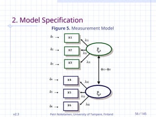
Figure 5. Measurement Model
57.
v2.3 Petri Nokelainen,University of Tampere, Finland 57 / 145
2. Model Specification
One can specify a model with different
methods, e.g., Bentler-Weeks or LISREL.
In Bentler-Weeks method every variable in the
model is either an IV or a DV.
The parameters to be estimated are
the regression coefficients and
the variances and the covariances of the independent
variables in the model. (Bentler, 1995.)
58.
v2.3 Petri Nokelainen,University of Tampere, Finland 58 / 145
2. Model Specification
Specification of the confirmatory factor model
requires making formal and explicit statements
about
the number of common factors,
the number of observed variables,
the variances and covariances among the common factors,
the relationships among observed variables and latent
factors,
the relationships among residual variables and
the variances and covariances among the residual
variables. (Jöreskog et al., 1989.)
59.
v2.3 Petri Nokelainen,University of Tampere, Finland 59 / 145
2. Model Specification
We start model specification by describing
factor equations in a two-factor model: a
Supportive Management factor (x1 – x3)
and a Functional Group factor (x4 – x6), see
Figure 5.
Note that the observed variables do not have
direct links to all latent factors.
60.
v2.3 Petri Nokelainen,University of Tampere, Finland 60 / 145
2. Model Specification
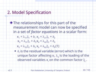
The relationships for this part of the
measurement model can now be specified
in a set of factor equations in a scalar form:
x1 = 111 + 1 x2 = 211 + 2
x3 = 311 + 3 x4 = 422 + 4
x5 = 522 + 5 x6 = 622 + 6 (1)
i is the residual variable (error) which is the
unique factor affecting xi. ij is the loading of the
observed variables xi on the common factor j .
61.
v2.3 Petri Nokelainen,University of Tampere, Finland 61 / 145
2. Model Specification
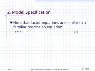
Note that factor equations are similar to a
familiar regression equation:
Y = X + (2)
62.
v2.3 Petri Nokelainen,University of Tampere, Finland 62 / 145
2. Model Specification
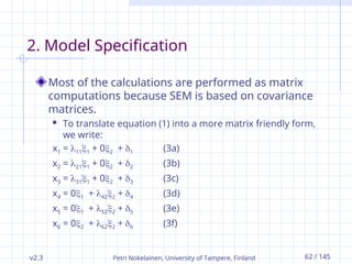
Most of the calculations are performed as matrix
computations because SEM is based on covariance
matrices.
To translate equation (1) into a more matrix friendly form,
we write:
x1 = 111 + 02 + 1 (3a)
x2 = 211 + 02 + 2 (3b)
x3 = 311 + 02 + 3 (3c)
x4 = 01 + 422 + 4 (3d)
x5 = 01 + 522 + 5 (3e)
x6 = 02 + 622 + 6 (3f)
63.
v2.3 Petri Nokelainen,University of Tampere, Finland 63 / 145
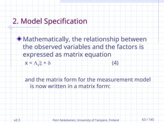
2. Model Specification
Mathematically, the relationship between
the observed variables and the factors is
expressed as matrix equation
x = x + (4)
and the matrix form for the measurement model
is now written in a matrix form:
64.
v2.3 Petri Nokelainen,University of Tampere, Finland 64 / 145
2. Model Specification
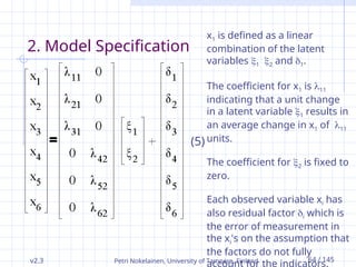
(5)
x1 is defined as a linear
combination of the latent
variables 1 2 and 1.
The coefficient for x1 is 11
indicating that a unit change
in a latent variable 1 results in
an average change in x1 of 11
units.
The coefficient for 2 is fixed to
zero.
Each observed variable xi has
also residual factor i which is
the error of measurement in
the xi's on the assumption that
the factors do not fully
account for the indicators.
65.
v2.3 Petri Nokelainen,University of Tampere, Finland 65 / 145
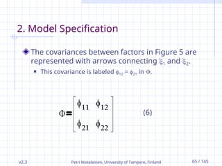
2. Model Specification
The covariances between factors in Figure 5 are
represented with arrows connecting 1 and 2.
This covariance is labeled 12 = 21 in .
(6)
66.
v2.3 Petri Nokelainen,University of Tampere, Finland 66 / 145
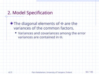
2. Model Specification
The diagonal elements of are the
variances of the common factors.
Variances and covariances among the error
variances are contained in .
67.
v2.3 Petri Nokelainen,University of Tampere, Finland 67 / 145
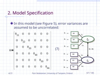
2. Model Specification
In this model (see Figure 5), error variances are
assumed to be uncorrelated:
(7)
68.
v2.3 Petri Nokelainen,University of Tampere, Finland 68 / 145
2. Model Specification
Because the factor equation (4) cannot be
directly estimated, the covariance structure
of the model is examined.
Matrix contains the structure of
covariances among the observed variables
after multiplying equation (4) by its
transpose
= E(xx') (8)
and taking expectations
= E[(+) (+)'] (9)
69.
v2.3 Petri Nokelainen,University of Tampere, Finland 69 / 145
2. Model Specification
Next we apply the matrix algebral
information that the transpose of a sum
matrices is equal to the sum of the
transpose of the matrices, and the
transpose of a product of matrices is the
product of the transposes in reverse order
(see Backhouse et al., 1989):
= E[(+) (''+')] (10)
70.
v2.3 Petri Nokelainen,University of Tampere, Finland 70 / 145
2. Model Specification
Applying the distributive property for matrices
we get
= E['' + ' + '' + '] (11)
Next we take expectations
= E[''] + E['] + E[''] + E['](12)
71.
v2.3 Petri Nokelainen,University of Tampere, Finland 71 / 145
2. Model Specification
Since the values of the parameters in matrix
are constant, we can write
= E['] ' + E['] + E['] ' + E['] (13)
72.
v2.3 Petri Nokelainen,University of Tampere, Finland 72 / 145
2. Model Specification
Since E['] = , ['] = , and and are
uncorrelated, previous equation can be simplified to
covariance equation:
= ' + (14)
The left side of the equation contains the number of
unique elements q(q+1)/2 in matrix .
The right side contains qs + s(s+1)/2 + q(q+1)/2
unknown parameters from the matrices , , and
.
Unknown parameters have been tied to the
population variances and covariances among the
observed variables which can be directly estimated
with sample data.
73.
v2.3 Petri Nokelainen,University of Tampere, Finland 73 / 145
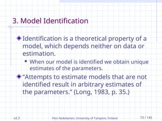
3. Model Identification
Identification is a theoretical property of a
model, which depends neither on data or
estimation.
When our model is identified we obtain unique
estimates of the parameters.
“Attempts to estimate models that are not
identified result in arbitrary estimates of
the parameters.” (Long, 1983, p. 35.)
74.
v2.3 Petri Nokelainen,University of Tampere, Finland 74 / 145
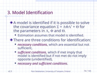
3. Model Identification
A model is identified if it is possible to solve
the covariance equation = ' + for
the parameters in , and .
Estimation assumes that model is identified.
There are three conditions for identification:
necessary conditions, which are essential but not
sufficient,
sufficient conditions, which if met imply that
model is identified but if not met do not imply
opposite (unidentified),
necessary and sufficient conditions.
75.
v2.3 Petri Nokelainen,University of Tampere, Finland 75 / 145
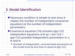
3. Model Identification
Necessary condition is simple to test since it
relates the number of independent covariance
equations to the number of independent
parameters.
Covariance equation (14) contains q(q+1)/2
independent equations and qs + s(s+1)/2 +
q(q+1)/2 possible independent parameters in ,
and .
Number of independent, unconstrained parameters of
the model must be less than or equal to q(q+1)/2.
76.
v2.3 Petri Nokelainen,University of Tampere, Finland 76 / 145
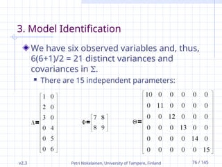
3. Model Identification
We have six observed variables and, thus,
6(6+1)/2 = 21 distinct variances and
covariances in .
There are 15 independent parameters:
77.
v2.3 Petri Nokelainen,University of Tampere, Finland 77 / 145
3. Model Identification
Since the number of independent
parameters is smaller than the independent
covariance equations (15<21), the necessary
condition for identification is satisfied.
78.
v2.3 Petri Nokelainen,University of Tampere, Finland 78 / 145
3. Model Identification
The most effective way to demonstrate that a
model is identified is to show that each of the
parameters can be solved in terms of the
population variances and covariances of the
observed variables.
Solving covariance equations is time-consuming
and there are other 'recipe-like' solutions.
79.
v2.3 Petri Nokelainen,University of Tampere, Finland 79 / 145
3. Model Identification
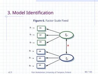
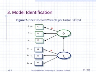
We gain constantly an identified model if
each observed variable in the model measures
only one latent factor and
factor scale is fixed (Figure 6) or one observed
variable per factor is fixed (Figure 7). (Jöreskog et
al., 1979, pp. 196-197; 1984.)
80.
v2.3 Petri Nokelainen,University of Tampere, Finland 80 / 145
3. Model Identification
Figure 6. Factor Scale Fixed
81.
v2.3 Petri Nokelainen,University of Tampere, Finland 81 / 145
3. Model Identification
Figure 7. One Observed Variable per Factor is Fixed
82.
v2.3 Petri Nokelainen,University of Tampere, Finland 82 / 145
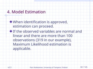
4. Model Estimation
When identification is approved,
estimation can proceed.
If the observed variables are normal and
linear and there are more than 100
observations (319 in our example),
Maximum Likelihood estimation is
applicable.
83.
v2.3 Petri Nokelainen,University of Tampere, Finland 83 / 145
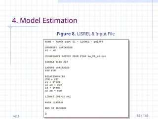
4. Model Estimation
Figure 8. LISREL 8 Input File
84.
v2.3 Petri Nokelainen,University of Tampere, Finland 84 / 145
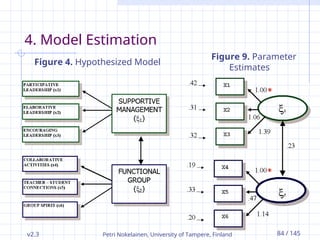
4. Model Estimation
Figure 9. Parameter
Estimates
Figure 4. Hypothesized Model
85.
v2.3 Petri Nokelainen,University of Tampere, Finland 85 / 145
Contents
Introduction
Path Analysis
Basic Concepts of Factor Analysis
Model Constructing
Model hypotheses
Model specification
Model identification
Model estimation
An Example of SEM: Commitment to Work and
Organization
Conclusions
References
86.
v2.3 Petri Nokelainen,University of Tampere, Finland 86 / 145
An Example of SEM: Commitment to
Work and Organization
Background
In 1998 RCVE undertook a growth-oriented
atmosphere study in a Finnish polytechnic
institute for higher education (later referred as
'organization').
The organization is a training and development
centre in the field of vocational education.
87.
v2.3 Petri Nokelainen,University of Tampere, Finland 87 / 145
An Example of SEM: Commitment to
Work and Organization
Background
In addition to teacher education, this organization
promotes vocational education in Finland through
developing vocational institutions and by offering
their personnel a variety of training programmes
which are tailored to their individual needs.
The objective of the study was to obtain
information regarding the current attitudes of
teachers of the organization to their commitment
to working environment (e.g., O'Neill et al., 1998).
88.
v2.3 Petri Nokelainen,University of Tampere, Finland 88 / 145
An Example of SEM: Commitment to
Work and Organization
DV (Eta1
1
) Commitment to
Work and Organization
COM Commitment to work
and organization
CO
IV1
(Xi1
1
) Supportive
Management
SUP Participative
Leadership
PAR
Elaborative Leadership ELA
Encouraging
Leadership
ENC
IV2
(Xi2
2
) Functional Group FUN Collaborative
Activities
COL
Teacher – Student
Connections
CON
Group Spirit SPI
IV3
(Xi3
3
) Stimulating Job STI Inciting Values INC
Job Value VAL
Influence on Job INF
Table 6. Dimensions of the Commitment to Work and Organization Model
89.
v2.3 Petri Nokelainen,University of Tampere, Finland 89 / 145
An Example of SEM: Commitment to
Work and Organization
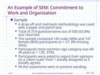
Sample
A drop-off and mail-back methodology was used
with a paper and pencil test.
Total of 319 questionnaires out of 500 (63.8%)
was returned.
The sample contained 145 male (46%) and 147
female (46%) participants (n = 27, 8% missing
data).
Participants most common age category was 40-
49 years (n = 120, 37%).
Participants were asked to report their opinions
on a ‘Likert scale’ from 1 (totally disagree) to 5
(totally agree).
All the statements were in positive wording.
90.
v2.3 Petri Nokelainen,University of Tampere, Finland 90 / 145
An Example of SEM: Commitment to
Work and Organization
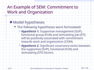
Model hypotheses
The following hypotheses were formulated:
Hypothesis 1. Supportive management (SUP),
functional group (FUN) and stimulating job (STI)
will be positively associated with commitment
towards work and organization (COM).
Hypothesis 2. Significant covariance exists between
the supportive (SUP), functional (FUN) and
stimulating (STI) factors.
91.
v2.3 Petri Nokelainen,University of Tampere, Finland 91 / 145
An Example of SEM: Commitment to
Work and Organization
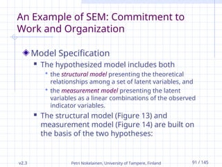
Model Specification
The hypothesized model includes both
the structural model presenting the theoretical
relationships among a set of latent variables, and
the measurement model presenting the latent
variables as a linear combinations of the observed
indicator variables.
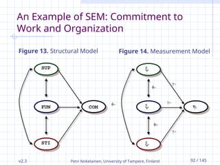
The structural model (Figure 13) and
measurement model (Figure 14) are built on
the basis of the two hypotheses:
92.
v2.3 Petri Nokelainen,University of Tampere, Finland 92 / 145
An Example of SEM: Commitment to
Work and Organization
Figure 13. Structural Model Figure 14. Measurement Model
93.
v2.3 Petri Nokelainen,University of Tampere, Finland 93 / 145
An Example of SEM: Commitment to
Work and Organization
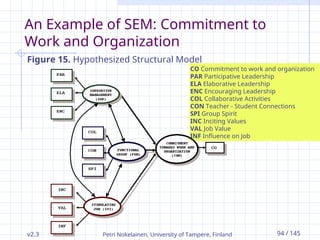
The hypothesized model is presented in Figure
15:
A Commitment towards work and organization
(COM 1) with
CO (Y1),
A Supportive Management (SUP 1) with
PAR (X1) ELA (X2) and ENC (X3),
A Functional group (FUN 2) with
COL (X4) CON (X5) and SPI (X6), and
A Stimulating work (STI 3) with
INC (X7) VAL (X8) and INF (X9).
94.
v2.3 Petri Nokelainen,University of Tampere, Finland 94 / 145
An Example of SEM: Commitment to
Work and Organization
Figure 15. Hypothesized Structural Model
CO Commitment to work and organization
PAR Participative Leadership
ELA Elaborative Leadership
ENC Encouraging Leadership
COL Collaborative Activities
CON Teacher - Student Connections
SPI Group Spirit
INC Inciting Values
VAL Job Value
INF Influence on Job
95.
v2.3 Petri Nokelainen,University of Tampere, Finland 95 / 145
An Example of SEM: Commitment to
Work and Organization
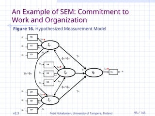
Figure 16. Hypothesized Measurement Model
96.
v2.3 Petri Nokelainen,University of Tampere, Finland 96 / 145
An Example of SEM: Commitment to
Work and Organization
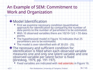
Model Identification
First we examine necessary condition (quantitative
approach) for identification by comparing the number of
data points to the number of parameters to be estimated.
With 10 observed variables there are 10(10+1)/2 = 55 data
points.
The hypothesized model in Figure 16 indicates that 25
parameters are to be estimated.
The model is over-identified with df 30 (55 - 25).
The necessary and sufficient condition for
identification is filled when each observed variable
measures one and only one latent variable and one
observed variable per latent factor is fixed
(Jöreskog, 1979, pp. 191-197).
Fixed variables are indicated with red asterisks in Figure 16.
97.
v2.3 Petri Nokelainen,University of Tampere, Finland 97 / 145
An Example of SEM: Commitment to
Work and Organization
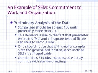
Preliminary Analysis of the Data
Sample size should be at least 100 units,
preferably more than 200.
This demand is due to the fact that parameter
estimates (ML) and chi-square tests of fit are
sensitive to sample size.
One should notice that with smaller sample
sizes the generalized least-squares method
(GLS) is still applicable.
Our data has 319 observations, so we may
continue with standard settings.
98.
v2.3 Petri Nokelainen,University of Tampere, Finland 98 / 145
An Example of SEM: Commitment to
Work and Organization
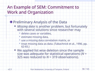
Preliminary Analysis of the Data
Missing data is another problem, but fortunately
with several solutions since researcher may
delete cases or variables,
estimate missing data,
use a missing data correlation matrix, or
treat missing data as data. (Tabachnick et al., 1996, pp.
62-65.)
We applied list wise deletion since the sample
size was adequate for statistical operations (N =
325 was reduced to N = 319 observations).
99.
v2.3 Petri Nokelainen,University of Tampere, Finland 99 / 145
An Example of SEM: Commitment to
Work and Organization
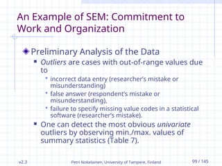
Preliminary Analysis of the Data
Outliers are cases with out-of-range values due
to
incorrect data entry (researcher’s mistake or
misunderstanding)
false answer (respondent’s mistake or
misunderstanding),
failure to specify missing value codes in a statistical
software (researcher’s mistake).
One can detect the most obvious univariate
outliers by observing min./max. values of
summary statistics (Table 7).
100.
v2.3 Petri Nokelainen,University of Tampere, Finland 100 / 145
An Example of SEM: Commitment to
Work and Organization
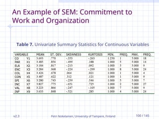
Table 7. Univariate Summary Statistics for Continuous Variables
101.
v2.3 Petri Nokelainen,University of Tampere, Finland 101 / 145
An Example of SEM: Commitment to
Work and Organization
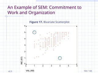
Preliminary Analysis of the Data
A more exact (but tedious!) way to identify
possible bivariate outliers is to produce scatter
plots.
Figure 17 is produced with SPSS (Graphs – Interactive
– Dot).
102.
v2.3 Petri Nokelainen,University of Tampere, Finland 102 / 145
An Example of SEM: Commitment to
Work and Organization
Figure 17. Bivariate Scatterplot
103.
v2.3 Petri Nokelainen,University of Tampere, Finland 103 / 145
An Example of SEM: Commitment to
Work and Organization
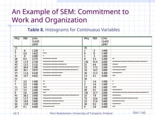
Preliminary Analysis of the Data
Multivariate normality is the assumption that
each variable and all linear combinations of the
variables are normally distributed.
When previously described assumption is met,
the residuals are also normally distributed and
independent.
This is important when carrying out SEM
analysis.
Histograms provide a good graphical look into
data (Table 8) to seek for skewness.
104.
v2.3 Petri Nokelainen,University of Tampere, Finland 104 / 145
An Example of SEM: Commitment to
Work and Organization
Table 8. Histograms for Continuous Variables
105.
v2.3 Petri Nokelainen,University of Tampere, Finland 105 / 145
An Example of SEM: Commitment to
Work and Organization
Preliminary Analysis of the Data
By examining the Table 9 we notice that
distribution of variables X1 and X9 is negatively
skewed.
Furthermore, observing skewness values (Table
9) we see that bias is statistically significant (X1=
-2.610, p = .005; X9= -2.657, p=.004 and X7= -
2.900, p = .002).
106.
v2.3 Petri Nokelainen,University of Tampere, Finland 106 / 145
An Example of SEM: Commitment to Work
and Organization
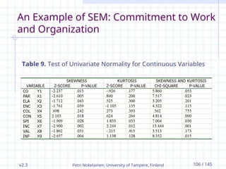
Table 9. Test of Univariate Normality for Continuous Variables
107.
v2.3 Petri Nokelainen,University of Tampere, Finland 107 / 145
An Example of SEM: Commitment to
Work and Organization
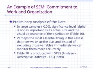
Preliminary Analysis of the Data
In large samples (>200), significance level (alpha)
is not as important as its actual size and the
visual appearance of the distribution (Table 10).
Perhaps the most essential thing in this case is
that now we know the bias and instead of
excluding those variables immediately we can
monitor them more accurately.
Table 10 is produced with SPSS (Analyze –
Descriptive Statistics – Q-Q Plots).
108.
v2.3 Petri Nokelainen,University of Tampere, Finland 108 / 145
An Example of SEM: Commitment to Work
and Organization
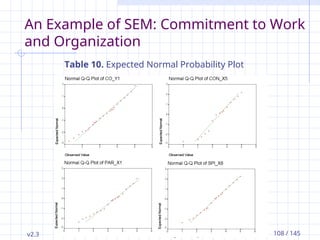
Table 10. Expected Normal Probability Plot
109.
v2.3 Petri Nokelainen,University of Tampere, Finland 109 / 145
An Example of SEM: Commitment to Work
and Organization
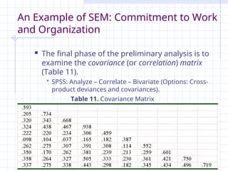
The final phase of the preliminary analysis is to
examine the covariance (or correlation) matrix
(Table 11).
SPSS: Analyze – Correlate – Bivariate (Options: Cross-
product deviances and covariances).
Table 11. Covariance Matrix
110.
v2.3 Petri Nokelainen,University of Tampere, Finland 110 / 145
An Example of SEM: Commitment to
Work and Organization
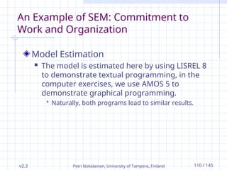
Model Estimation
The model is estimated here by using LISREL 8
to demonstrate textual programming, in the
computer exercises, we use AMOS 5 to
demonstrate graphical programming.
Naturally, both programs lead to similar results.
111.
v2.3 Petri Nokelainen,University of Tampere, Finland 111 / 145
An Example of SEM: Commitment to Work
and Organization
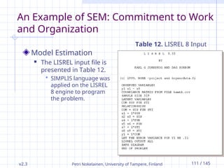
Model Estimation
The LISREL input file is
presented in Table 12.
SIMPLIS language was
applied on the LISREL
8 engine to program
the problem.
Table 12. LISREL 8 Input
112.
v2.3 Petri Nokelainen,University of Tampere, Finland 112 / 145
An Example of SEM: Commitment to Work
and Organization
Model Estimation
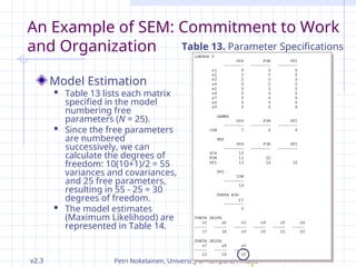
Table 13 lists each matrix
specified in the model
numbering free
parameters (N = 25).
Since the free parameters
are numbered
successively, we can
calculate the degrees of
freedom: 10(10+1)/2 = 55
variances and covariances,
and 25 free parameters,
resulting in 55 - 25 = 30
degrees of freedom.
The model estimates
(Maximum Likelihood) are
represented in Table 14.
Table 13. Parameter Specifications
113.
v2.3 Petri Nokelainen,University of Tampere, Finland 113 / 145
An Example of SEM: Commitment to Work
and Organization
Model Estimation
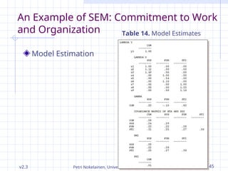
Table 14. Model Estimates
114.
v2.3 Petri Nokelainen,University of Tampere, Finland 114 / 145
An Example of SEM: Commitment to
Work and Organization
Model Estimation
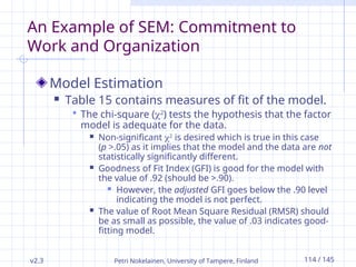
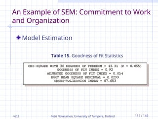
Table 15 contains measures of fit of the model.
The chi-square (2
) tests the hypothesis that the factor
model is adequate for the data.
Non-significant 2
is desired which is true in this case
(p >.05) as it implies that the model and the data are not
statistically significantly different.
Goodness of Fit Index (GFI) is good for the model with
the value of .92 (should be >.90).
However, the adjusted GFI goes below the .90 level
indicating the model is not perfect.
The value of Root Mean Square Residual (RMSR) should
be as small as possible, the value of .03 indicates good-
fitting model.
115.
v2.3 Petri Nokelainen,University of Tampere, Finland 115 / 145
An Example of SEM: Commitment to Work
and Organization
Model Estimation
Table 15. Goodness of Fit Statistics
116.
v2.3 Petri Nokelainen,University of Tampere, Finland 116 / 145
An Example of SEM: Commitment to
Work and Organization
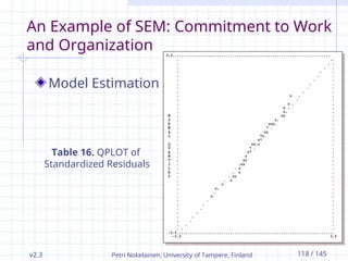
Model Estimation
Standardized residuals are residuals divided by
their standard errors (Jöreskog, 1989, p. 103).
All residuals have moderate values (min. -2.81,
max. 2.28), which means that the model
estimates adequately relationships between
variables.
QPLOT of standardized residuals is presented
in Table 16 where a x represents a single point,
and an * multiple points.
117.
v2.3 Petri Nokelainen,University of Tampere, Finland 117 / 145
An Example of SEM: Commitment to
Work and Organization
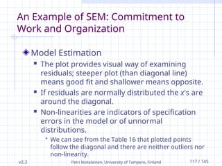
Model Estimation
The plot provides visual way of examining
residuals; steeper plot (than diagonal line)
means good fit and shallower means opposite.
If residuals are normally distributed the x's are
around the diagonal.
Non-linearities are indicators of specification
errors in the model or of unnormal
distributions.
We can see from the Table 16 that plotted points
follow the diagonal and there are neither outliers nor
non-linearity.
118.
v2.3 Petri Nokelainen,University of Tampere, Finland 118 / 145
An Example of SEM: Commitment to Work
and Organization
Model Estimation
Table 16. QPLOT of
Standardized Residuals
119.
v2.3 Petri Nokelainen,University of Tampere, Finland 119 / 145
An Example of SEM: Commitment to
Work and Organization
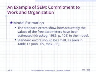
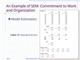
Model Estimation
The standard errors show how accurately the
values of the free parameters have been
estimated (Jöreskog, 1989, p. 105) in the model.
Standard errors should be small, as seen in
Table 17 (min. .05, max. .35).
120.
v2.3 Petri Nokelainen,University of Tampere, Finland 120 / 145
An Example of SEM: Commitment to Work
and Organization
Table 17. Standard Errors
Model Estimation
121.
v2.3 Petri Nokelainen,University of Tampere, Finland 121 / 145
An Example of SEM: Commitment to
Work and Organization
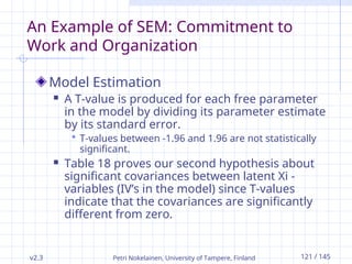
Model Estimation
A T-value is produced for each free parameter
in the model by dividing its parameter estimate
by its standard error.
T-values between -1.96 and 1.96 are not statistically
significant.
Table 18 proves our second hypothesis about
significant covariances between latent Xi -
variables (IV’s in the model) since T-values
indicate that the covariances are significantly
different from zero.
122.
v2.3 Petri Nokelainen,University of Tampere, Finland 122 / 145
An Example of SEM: Commitment to Work
and Organization
Model Estimation
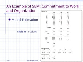
Table 18. T-values
123.
v2.3 Petri Nokelainen,University of Tampere, Finland 123 / 145
An Example of SEM: Commitment to
Work and Organization
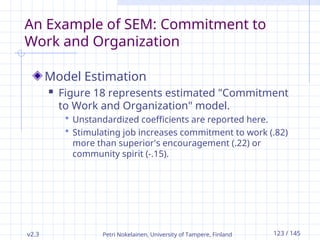
Model Estimation
Figure 18 represents estimated "Commitment
to Work and Organization" model.
Unstandardized coefficients are reported here.
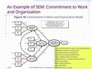
Stimulating job increases commitment to work (.82)
more than superior's encouragement (.22) or
community spirit (-.15).
124.
v2.3 Petri Nokelainen,University of Tampere, Finland 124 / 145
An Example of SEM: Commitment to Work
and Organization
Figure 18. Commitment to Work and Organization Model
CO Commitment to work and organization
PAR Participative Leadership
ELA Elaborative Leadership
ENC Encouraging Leadership
COL Collaborative Activities
CON Teacher - Student Connections
SPI Group Spirit
INC Inciting Values
VAL Job Value
INF Influence on Job
125.
v2.3 Petri Nokelainen,University of Tampere, Finland 125 / 145
An Example of SEM: Commitment to
Work and Organization
Model Estimation
Figures 19 and 20 represent the same model
before and after AMOS 5 analysis.
AMOS uses SPSS data matrix as an input file.
126.
v2.3 Petri Nokelainen,University of Tampere, Finland 126 / 145
An Example of SEM: Commitment to Work
and Organization
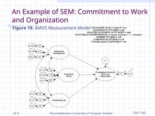
Figure 19. AMOS Measurement Model
127.
v2.3 Petri Nokelainen,University of Tampere, Finland 127 / 145
An Example of SEM: Commitment to Work
and Organization
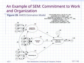
Figure 20. AMOS Estimation Model
128.
v2.3 Petri Nokelainen,University of Tampere, Finland 128 / 145
An Example of SEM: Commitment to
Work and Organization
Model Estimation
Naturally, both LISREL and AMOS produce
similar results:
Unstandardized coefficients are reported here.
Stimulating job increases in both models
commitment to work (.82/.68) more than superior's
encouragement (.22/.15) or community spirit
(-.15/-.14).
129.
v2.3 Petri Nokelainen,University of Tampere, Finland 129 / 145
Contents
Introduction
Path Analysis
Basic Concepts of Factor Analysis
Model Constructing
Model hypotheses
Model specification
Model identification
Model estimation
An Example of SEM: Commitment to Work and
Organization
Conclusions
References
130.
v2.3 Petri Nokelainen,University of Tampere, Finland 130 / 145
Conclusions
SEM has proven to be a very versatile statistical
toolbox for educational researchers when used to
confirm theoretical structures.
Perhaps the greatest strength of SEM is the
requirement of a prior knowledge of the
phenomena under examination.
In practice, this means that the researcher is testing a
theory which is based on an exact and explicit plan or
design.
One may also notice that relationships among factors
examined are free of measurement error because it has
been estimated and removed, leaving only common
variance.
Very complex and multidimensional structures can be
measured with SEM; in that case SEM is the only linear
analysis method that allows complete and simultaneous
tests of all relationships.
131.
v2.3 Petri Nokelainen,University of Tampere, Finland 131 / 145
Conclusions
Disadvantages of SEM are also simple to point out.
Researcher must be very careful with the study design
when using SEM for exploratory work.
As mentioned earlier, the use of the term ‘causal modeling’
referring to SEM is misleading because there is nothing
causal, in the sense of inferring causality, about the use of
SEM.
SEM's ability to analyze more complex relationships
produces more complex models: Statistical language has
turned into jargon due to vast supply of analytic software
(LISREL, EQS, AMOS).
When analyzing scientific reports methodologically based
on SEM, usually a LISREL model, one notices that they lack
far too often decent identification inspection which is a
prerequisite to parameter estimation.
132.
v2.3 Petri Nokelainen,University of Tampere, Finland 132 / 145
Conclusions
Overgeneralization is always a problem – but
specifically with SEM one must pay extra
attention when interpreting causal relationships
since multivariate normality of the data is
assumed.
This is a severe limitation of linear analysis in general
because the reality is seldom linear.
We must also point out that SEM is based on
covariances that are not stable when estimated
from small (<200 observation) samples.
On the other hand, too large (>200 observations)
sample size is also a reported problem (e.g.,
Bentler et al., 1983) of the significance of 2
.
133.
v2.3 Petri Nokelainen,University of Tampere, Finland 133 / 145
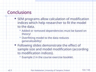
Conclusions
SEM programs allow calculation of modification
indices which help researcher to fit the model
to the data.
Added or removed dependencies must be based on
theory!
Overfitting model to the data reduces
generalizability!
Following slides demonstrate the effect of
sample size and model modification (according
to modification indices).
Example 2 in the course exercise booklet.
v2.3 Petri Nokelainen,University of Tampere, Finland 135 / 145
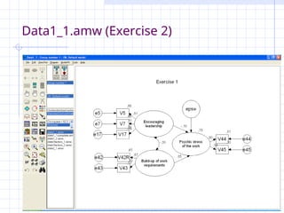
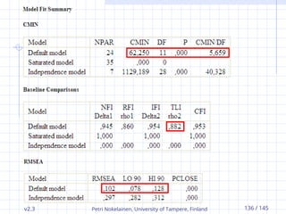
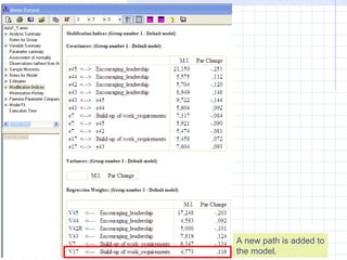
Data1_1.amw (Exercise 2)
Large sample (n=447) produces biased
2
/df and p values (both too large).
Model fit indices are satisfactory at best
(RMSEA > .10, TLI <.90).
As there are missing values in the data,
calculation of modification indices is not
allowed (in AMOS).
v2.3 Petri Nokelainen,University of Tampere, Finland 137 / 145
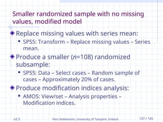
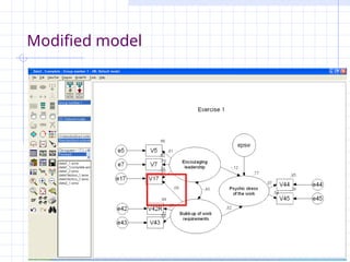
Smaller randomized sample with no missing
values, modified model
Replace missing values with series mean:
SPSS: Transform – Replace missing values – Series
mean.
Produce a smaller (n=108) randomized
subsample:
SPSS: Data – Select cases – Random sample of
cases – Approximately 20% of cases.
Produce modification indices analysis:
AMOS: View/set – Analysis properties –
Modification indices.
138.
v2.3 Petri Nokelainen,University of Tampere, Finland 138 / 145
A new path is added to
the model.
v2.3 Petri Nokelainen,University of Tampere, Finland 141 / 145
Contents
Introduction
Path Analysis
Basic Concepts of Factor Analysis
Model Constructing
Model hypotheses
Model specification
Model identification
Model estimation
An Example of SEM: Commitment to Work and
Organization
Conclusions
References
142.
v2.3 Petri Nokelainen,University of Tampere, Finland 142 / 145
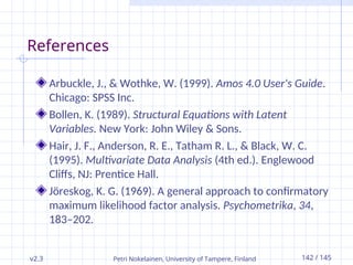
References
Arbuckle, J., & Wothke, W. (1999). Amos 4.0 User's Guide.
Chicago: SPSS Inc.
Bollen, K. (1989). Structural Equations with Latent
Variables. New York: John Wiley & Sons.
Hair, J. F., Anderson, R. E., Tatham R. L., & Black, W. C.
(1995). Multivariate Data Analysis (4th ed.). Englewood
Cliffs, NJ: Prentice Hall.
Jöreskog, K. G. (1969). A general approach to confirmatory
maximum likelihood factor analysis. Psychometrika, 34,
183–202.
143.
v2.3 Petri Nokelainen,University of Tampere, Finland 143 / 145
References
Kaplan, D. (2000). Structural Equation Modeling.
Thousand Oaks: Sage.
Long, J. (1983). Confirmatory Factor Analysis. California:
Sage.
Muthén, L., & Muthén, B. (2000). MPLUS User Manual.
Los Angeles: Muthén & Muthén.
Nokelainen, P., & Ruohotie, P. (1999). Structural Equation
Modeling in Professional Growth Research. In P. Ruohotie,
H. Tirri, P. Nokelainen, & T. Silander (Eds.), Modern
Modeling of Professional Growth, vol. 1 (pp. 121-154).
Hämeenlinna: RCVE.
144.
v2.3 Petri Nokelainen,University of Tampere, Finland 144 / 145
References
Nokelainen, P., & Ruohotie, P. (2009). Non-linear
Modeling of Growth Prerequisites in a Finnish Polytechnic
Institution of Higher Education. Journal of Workplace
Learning, 21(1), 36-57.
Pearl, J. (2000). Causality. New York: Cambridge University
Press.
Ruohotie, P. (1996). Professional Growth and
Development. In K. Leithwood et al. (Eds.), International
Handbook of Educational Leadership and Administration
(pp. 419-445). Dordrecht: Kluwer Academic Publishers.
Raykov, T., & Marcoulides, G. (2000). A First Course in
Structural Equation Modeling. Mahwah, NJ: Lawrence
Erlbaum Associates.
145.
v2.3 Petri Nokelainen,University of Tampere, Finland 145 / 145
References
Sager, J., Griffeth, R., & Hom, P. (1998). A Comparison of
Structural Models Representing Turnover Cognitions.
Journal of Vocational Behavior, 53, 254-273.
Schumacker, R. E., & Lomax, R. G. (2004). A Beginner's
Guide to Structural Equation Modeling (2nd ed.).
Mahwah, NJ: Lawrence Erlbaum Associates.
Tabachnick, B ., & Fidell, L. (1996). Using Multivariate
Statistics. New York: HarperCollins.
Wright, S. (1921). Correlation and Causation. Journal of
Agricultural Research, 20, 557-585.
Wright, S. (1934). The Method of Path Coefficients. The
Annals of Mathematical Statistics, 5, 161-215.
![Petri Nokelainen, University of Tampere, Finland 7 / 145
Introduction
Genetics S. Wright (1921): “Prior knowledge of
the causal relations is assumed as prerequisite
… [in linear structural modeling]”.
y = x +
“In an ideal experiment where we control X to x
and any other set Z of variables (not containing
X or Y) to z, the value of Y is given by x + ,
where is not a function of the settings x and z.”
(Pearl, 2000)
v2.3](https://image.slidesharecdn.com/structuralequationmodeling-250309171102-29b3b316/85/Structural-Equation-Modeling-concepts-and-applications-ppt-7-320.jpg)


![v2.3 Petri Nokelainen, University of Tampere, Finland 68 / 145
2. Model Specification
Because the factor equation (4) cannot be
directly estimated, the covariance structure
of the model is examined.
Matrix contains the structure of
covariances among the observed variables
after multiplying equation (4) by its
transpose
= E(xx') (8)
and taking expectations
= E[(+) (+)'] (9)](https://image.slidesharecdn.com/structuralequationmodeling-250309171102-29b3b316/85/Structural-Equation-Modeling-concepts-and-applications-ppt-68-320.jpg)
![v2.3 Petri Nokelainen, University of Tampere, Finland 69 / 145
2. Model Specification
Next we apply the matrix algebral
information that the transpose of a sum
matrices is equal to the sum of the
transpose of the matrices, and the
transpose of a product of matrices is the
product of the transposes in reverse order
(see Backhouse et al., 1989):
= E[(+) (''+')] (10)](https://image.slidesharecdn.com/structuralequationmodeling-250309171102-29b3b316/85/Structural-Equation-Modeling-concepts-and-applications-ppt-69-320.jpg)
![v2.3 Petri Nokelainen, University of Tampere, Finland 70 / 145
2. Model Specification
Applying the distributive property for matrices
we get
= E['' + ' + '' + '] (11)
Next we take expectations
= E[''] + E['] + E[''] + E['](12)](https://image.slidesharecdn.com/structuralequationmodeling-250309171102-29b3b316/85/Structural-Equation-Modeling-concepts-and-applications-ppt-70-320.jpg)
![v2.3 Petri Nokelainen, University of Tampere, Finland 71 / 145
2. Model Specification
Since the values of the parameters in matrix
are constant, we can write
= E['] ' + E['] + E['] ' + E['] (13)](https://image.slidesharecdn.com/structuralequationmodeling-250309171102-29b3b316/85/Structural-Equation-Modeling-concepts-and-applications-ppt-71-320.jpg)
![v2.3 Petri Nokelainen, University of Tampere, Finland 72 / 145
2. Model Specification
Since E['] = , ['] = , and and are
uncorrelated, previous equation can be simplified to
covariance equation:
= ' + (14)
The left side of the equation contains the number of
unique elements q(q+1)/2 in matrix .
The right side contains qs + s(s+1)/2 + q(q+1)/2
unknown parameters from the matrices , , and
.
Unknown parameters have been tied to the
population variances and covariances among the
observed variables which can be directly estimated
with sample data.](https://image.slidesharecdn.com/structuralequationmodeling-250309171102-29b3b316/85/Structural-Equation-Modeling-concepts-and-applications-ppt-72-320.jpg)


![[DSC Europe 25] Ivan Lukovic & Marija Djukic - From Data to Value: Why Maturi...](https://cdn.slidesharecdn.com/ss_thumbnails/ahrfps8xr6knowwhacxh-1-ivan-marija-dsc-2025-ld-v1-presentation-260115093812-be21adfc-thumbnail.jpg?width=640&height=640&fit=bounds)


