The document discusses the meaning of data in statistics, defining it as observations or outcomes from experiments. It categorizes data into qualitative and quantitative types, detailing various variable types such as discrete and continuous. Additionally, it explains levels of measurement, provides examples, and outlines steps for constructing frequency distributions.

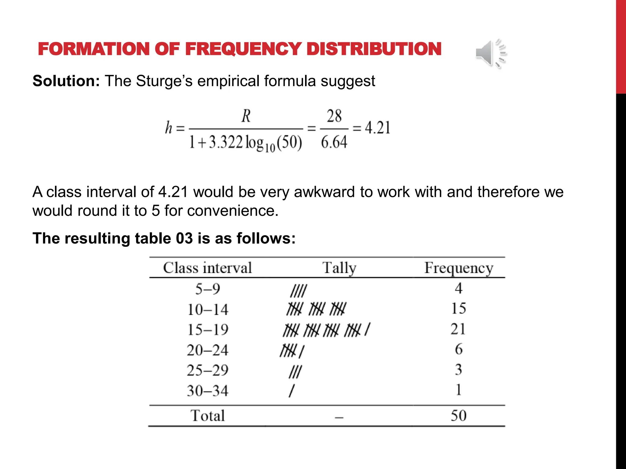
1. STATISTICS
DATA AND VARIABLE
WEEK-2

2. MEANING OF DATA
• Data are the observations or chance outcomes that occur in a planned
experiments or scientific investigations. They are the raw materials of statistics
and for all statistical purposes, we may define data as numbers whose common
characteristic is variability or variation.
• For example, among the male workers of an industry to know whether the
workers smoke or not. The answer may be recorded as 'yes' for those who
smoke and 'no' for those who do not smoke. Thus, all the workers of the industry
may be classified into two categories: smokers and non-smokers. The number of
smokers and non-smokers are numerical data, obtained through the process of
counting. We may further attempt to record their ages or measure their height
and thus obtain some numerical data on age and height. Some information may
be obtained simply by observing whether a particular event occurs or does not
occur. For example, we may observe whether a given day is rainy or sunny, a
man has blue eyes or brown eyes. All these information constitute data.

3. TYPES OF DATA
Statistical data may be broadly classified into two broad categories:
• Qualitative data:
Qualitative data are generated by assigning observations into various
independent categories and then counting the frequency of the
occurrences within these categories.
Example: Counting how many persons in a community are Muslims,
and how many of them are of other religions. Clearly the qualitative data
are those which can be stated or expressed in qualitative terms.

4. TYPES OF DATA
• Quantitative data:
Quantitative data are those which can be measured in quantitative units.
Here we are able to measure or note the actual magnitude of some
characteristics for each of the individuals or units under consideration.
Example: Measurement of height, weight, income, temperature, family
size or the number of street accidents over a specified period will all
result in quantitative data.

5. LEVEL OF MEASUREMENT
Measurement is essentially the task of assigning numbers to
observations according to certain rules. The way in which the numbers
are assigned to observations determines the scale of measurement
being used. The rule chosen for the assignment process, then, is the
key to which measurement scale is being used.
There are four levels of measurement. They are (a) Nominal level (b)
Ordinal level (c) Interval level and (d) Ratio level.
Each type of measurement has unique characteristics and implications
for the type of statistical procedures that can be used with it.

6. COMPARING THE DIFFERENT LEVELS OF MEASUREMENT
Scales Characteristics Examples
Nominal
Categories are homogeneous, mutually exclusive,
and no assumptions about ordered relationships
between categories made
 Sex of subject
 Eye color
 Religion
 Political affiliation
 Place of residence
 Room numbers etc
Ordinal
All of the above plus the categories can be rank-
ordered
 Examination grade
 Health status
 Level of education
 Rank in job
Interval
All of the above plus exact differences between
categories are specified and an arbitrary zero
point is assumed
 Temperature
 IQ test score
 Calendar time
Ratio
All of the above with the exception that a true zero
point is assumed
 Height
 Weight
 Fat consumed
 Wage

7. VARIABLE
• Variable: A variable is a characteristic or property, often but not
always quantitatively measured, containing two or more values or
categories that can vary from one individual to another.
• Example: Age, Sex, Height, Weight, Religion etc.

8. DIFFERENT TYPES OF VARIABLE
• Qualitative variable: A qualitative variable is a characteristic
that is not capable of being measured but can be categorized
to possess or not to possess some characteristics.
A few examples of qualitative variable are:
 Color of a garment (red, white, etc.).
 Bank account type (savings, current, fixed).
 Place of birth (rural, urban, sub-urban etc.),
 Sex (male, female).
 Frequency of visits (frequent, occasional, rare, never).
 Examination grade (A, B, C).
8

9. DIFFERENT TYPES OF VARIABLE
• Quantitative variable: A quantitative variable is one for
which the resulting observations are numeric and thus
possesses a natural ordering.
Examples of quantitative variables are:
 Sales volume in a department store
 Years of teaching experience of an individual
 Income of individuals
 Longevity of lives
 Day temperature.
9

10. DIFFERENT TYPES OF VARIABLE
• Discrete variable: A variable can take on only values at
isolated points along a scale of values, is called a discrete
variable.
Examples of discrete variables are:
 Family size
 Number of days absent from work for illness
 Number of shares in a business
 Number of automobiles imported during 1980–1990
 Number of units of an item in an inventory
 Number of assembled components found to be defective
 Number of typing errors in a document.
10

11. DIFFERENT TYPES OF VARIABLE
• Continuous variable: A continuous variable is one that
may take on infinite number of intermediate values along
a specified interval.
Examples of continuous variables are:
 Payoffs in business
 Waiting time in a bank counter
 Hourly average payment of factory workers
 Rainfall in millimeter recorded by meteorological office
 Height or weight of individuals.
11

12. PRESENTING DATA
A set of data even if modest in size, is often difficult to comprehend and interpret
directly in the form in which it is collected. Suppose a sample of 50 workers was
drawn from a business enterprise, which employed 500 workers. The researcher
collected such data as the workers’ age, level of education, wage, and their religion
by directly interviewing the workers. These are some of the personal characteristics
of the workers which the researcher needs to meet the objectives of a social
research. Having obtained the data, the most usual questions one might ask now:
a) How many of the workers are below 30 years of age? Over 50?
b) How many of them earn between 74 and 81 taka?
c) How many of them have secondary level of education?
d) Do most of the workers have large family size?
e) How many workers belong to minority group?
f) Are the workers frequent to remain absent from work?

13. FREQUENCY DISTRIBUTION
Frequency distribution: A frequency distribution is a set of mutually exclusive
classes or categories together with the frequency of occurrence of items, values
or observations in each class or category in a given set of data, presented
usually in a tabular form.

14. CONSTRUCTING FREQUENCY DISTRIBUTION
FOR QUALITATIVE DATA
Example: Construct a frequency distribution for the family size data presented
in below Table 01
Worker Family size Worker Family size Worker Family size
1 Small 18 Large 35 Medium
2 Large 19 Medium 36 Large
3 Small 20 Medium 37 Medium
4 Medium 21 Medium 38 Large
5 Large 22 Small 39 Medium
6 Medium 23 Small 40 Medium
7 Large 24 Medium 41 Medium
8 Small 25 Medium 42 Large
9 Large 26 Small 43 Large
10 Medium 27 Large 44 Medium
11 Large 28 Small 45 Medium
12 Small 29 Medium 46 Medium
13 Large 30 Large 47 Small
14 Medium 31 Medium 48 Small
15 Medium 32 Large 49 Medium
16 Medium 33 Medium 50 Medium
17 Large 34 Large

15. CONSTRUCTING FREQUENCY DISTRIBUTION
FOR QUALITATIVE DATA
Solution: The process follows the following steps:
 The first family in the order is ‘small’. The category, ‘small’ appears in the first column
of the table as a third entry. Put a tally mark against the family size ‘small’, which is
simply a left-slashed off-diagonal stroke ().
 Move on to the next entry, which is ‘large’. Enter this again by a tally mark against
the category ‘large’ appearing in the table.
 Repeat the above process until you have entered all the 50 items appearing in the
observed set shown in above table 01.
 In the process of tallying, when you have completed four tallies in a category, put the
fifth tally across the bunch of four by a diagonal slash to make a bunch of 5 tallies.
 Count the tallies for each category and put the number of tallies so counted in a
tabular form.

16. CONSTRUCTING FREQUENCY DISTRIBUTION
FOR QUALITATIVE DATA
The resulting tallies that appear below form our desired frequency
distribution of family size shown in below
Table 02: Frequency distribution of family size
The counts 16, 24, and 10 appearing in the second column of the table
are the class frequencies for the categories large, medium and small
respectively. The count 50 is the total frequency, which implies that we
have listed all 50 cases. Since the data are grouped into non-numerical
categories, the distribution is referred to as qualitative distribution.

17. STEPS IN CONSTRUCTING GROUPED DISTRIBUTION
The construction of such a distribution consists essentially of the following four
steps.
a) Decide on number of classes and the class widths in which the observations
are to be grouped.
b) Assign the observations to the appropriately chosen classes. This is called
tallying.
c) Count the number of observations falling in each class. These numbers are
the frequencies.
d) Display the results obtained in the above three steps in a table.
The resulting table is our desired frequency distribution.

18. HOW TO CHOOSE NUMBER OF CLASSES?
If the smallest value (S) and the largest value (L) in a data set are known, then as a
rule of thumb, the range , which shows the spread of the data, is divided by the class
width (h) to determine the approximate number of classes desired (k). In other words
An empirical rule suggested by Sturge to determine the number of classes is the “2
to the k rule”. This rule suggests that the number of classes should be the smallest
whole number k that makes the quantity 2k greater than or equal to the total number
of observations (N) in the data set (i.e. 2kN). Suppose a data set consists of N=50
observations. Then, since 25=32, which is smaller than N and 26=64, which is greater
than N, the Sturge’s rule dictates us to choose 6 classes, that is k=6.

19. HOW TO DECIDE ON THE CLASS INTERVAL?
This depends primarily on how the data look like. If k is empirically determined,
following Sturge, then a formula for h is
An empirical formula due to Sturge is also available, which has been found to
work well in many situations for choosing equal-spaced class interval (h):

20. FORMATION OF FREQUENCY DISTRIBUTION
Example: The number of complete days the workers were absent from their
work during the year preceding the inquiry are arranged below in an ascending
array:
5 8 9 9 10 10 10 10 11 11
12 12 12 13 13 13 14 14 14 15
15 15 15 16 16 16 16 17 17 17
17 18 18 18 18 18 19 19 19 19
20 21 21 22 23 24 26 27 29 33

21. FORMATION OF FREQUENCY DISTRIBUTION
Solution: The Sturge’s empirical formula suggest
A class interval of 4.21 would be very awkward to work with and therefore we
would round it to 5 for convenience.
The resulting table 03 is as follows:

22. THANK YOU