This document provides an introduction to SQL and the Oracle database system. It begins with an overview of database tables, columns, and data types. It then covers SQL queries, including selecting columns and tuples, aggregate functions, and string operations. The document also discusses data definition, modification, and integrity constraints and triggers in SQL.
![1 SQL – Structured Query Language
1.1 Tables
In relational database systems (DBS) data are represented using tables (relations). A query
issued against the DBS also results in a table. A table has the following structure:
Column 1 Column 2 . . . Column n
←− Tuple (or Record)
... ... ... ...
A table is uniquely identified by its name and consists of rows that contain the stored informa-
tion, each row containing exactly one tuple (or record ). A table can have one or more columns.
A column is made up of a column name and a data type, and it describes an attribute of the
tuples. The structure of a table, also called relation schema, thus is defined by its attributes.
The type of information to be stored in a table is defined by the data types of the attributes
at table creation time.
SQL uses the terms table, row, and column for relation, tuple, and attribute, respectively. In
this tutorial we will use the terms interchangeably.
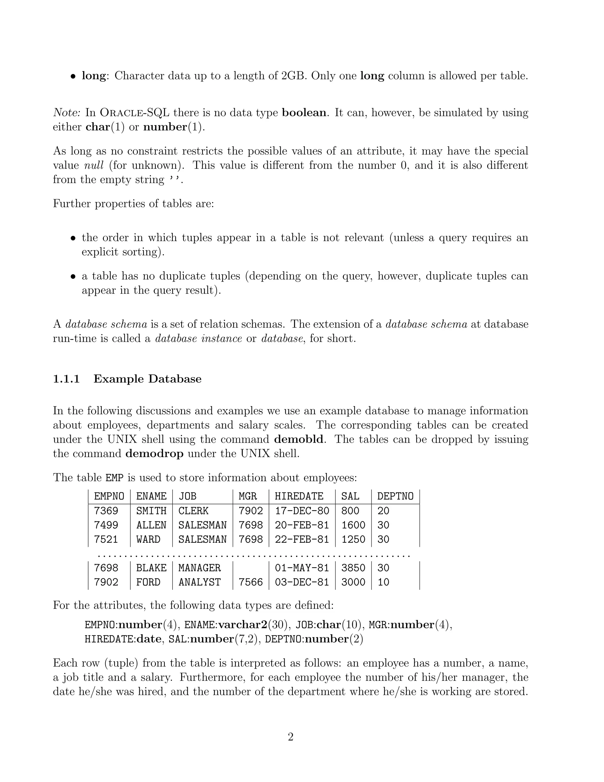
A table can have up to 254 columns which may have different or same data types and sets of
values (domains), respectively. Possible domains are alphanumeric data (strings), numbers and
date formats. Oracle offers the following basic data types:
• char(n): Fixed-length character data (string), n characters long. The maximum size for
n is 255 bytes (2000 in Oracle8). Note that a string of type char is always padded on
right with blanks to full length of n. ( can be memory consuming).
Example: char(40)
• varchar2(n): Variable-length character string. The maximum size for n is 2000 (4000 in
Oracle8). Only the bytes used for a string require storage. Example: varchar2(80)
• number(o, d): Numeric data type for integers and reals. o = overall number of digits, d
= number of digits to the right of the decimal point.
Maximum values: o =38, d= −84 to +127. Examples: number(8), number(5,2)
Note that, e.g., number(5,2) cannot contain anything larger than 999.99 without result-
ing in an error. Data types derived from number are int[eger], dec[imal], smallint
and real.
• date: Date data type for storing date and time.
The default format for a date is: DD-MMM-YY. Examples: ’13-OCT-94’, ’07-JAN-98’
1](https://image.slidesharecdn.com/cfakepathkunalboss-226-1b02c961-9cd4-4a44-ae8a-48f5f1c614ab-091113025135-phpapp01/75/SQL-3-2048.jpg)
![The table DEPT stores information about departments (number, name, and location):
DEPTNO DNAME LOC
10 STORE CHICAGO
20 RESEARCH DALLAS
30 SALES NEW YORK
40 MARKETING BOSTON
Finally, the table SALGRADE contains all information about the salary scales, more precisely, the
maximum and minimum salary of each scale.
GRADE LOSAL HISAL
1 700 1200
2 1201 1400
3 1401 2000
4 2001 3000
5 3001 9999
1.2 Queries (Part I)
In order to retrieve the information stored in the database, the SQL query language is used. In
the following we restrict our attention to simple SQL queries and defer the discussion of more
complex queries to Section 1.5
In SQL a query has the following (simplified) form (components in brackets [ ] are optional):
select [distinct] column(s)
from table
[ where condition ]
[ order by column(s) [asc|desc] ]
1.2.1 Selecting Columns
The columns to be selected from a table are specified after the keyword select. This operation
is also called projection. For example, the query
select LOC, DEPTNO from DEPT;
lists only the number and the location for each tuple from the relation DEPT. If all columns
should be selected, the asterisk symbol “∗” can be used to denote all attributes. The query
select ∗ from EMP;
retrieves all tuples with all columns from the table EMP. Instead of an attribute name, the select
clause may also contain arithmetic expressions involving arithmetic operators etc.
select ENAME, DEPTNO, SAL ∗ 1.55 from EMP;
3](https://image.slidesharecdn.com/cfakepathkunalboss-226-1b02c961-9cd4-4a44-ae8a-48f5f1c614ab-091113025135-phpapp01/75/SQL-5-2048.jpg)
![For the different data types supported in Oracle, several operators and functions are provided:
• for numbers: abs, cos, sin, exp, log, power, mod, sqrt, +, −, ∗, /, . . .
• for strings: chr, concat(string1, string2), lower, upper, replace(string, search string,
replacement string), translate, substr(string, m, n), length, to date, . . .
• for the date data type: add month, month between, next day, to char, . . .
The usage of these operations is described in detail in the SQL*Plus help system (see also
Section 2).
Consider the query
select DEPTNO from EMP;
which retrieves the department number for each tuple. Typically, some numbers will appear
more than only once in the query result, that is, duplicate result tuples are not automatically
eliminated. Inserting the keyword distinct after the keyword select, however, forces the
elimination of duplicates from the query result.
It is also possible to specify a sorting order in which the result tuples of a query are displayed.
For this the order by clause is used and which has one or more attributes listed in the select
clause as parameter. desc specifies a descending order and asc specifies an ascending order
(this is also the default order). For example, the query
select ENAME, DEPTNO, HIREDATE from EMP;
from EMP
order by DEPTNO [asc], HIREDATE desc;
displays the result in an ascending order by the attribute DEPTNO. If two tuples have the same
attribute value for DEPTNO, the sorting criteria is a descending order by the attribute values of
HIREDATE. For the above query, we would get the following output:
ENAME DEPTNO HIREDATE
FORD 10 03-DEC-81
SMITH 20 17-DEC-80
BLAKE 30 01-MAY-81
WARD 30 22-FEB-81
ALLEN 30 20-FEB-81
...........................
1.2.2 Selection of Tuples
Up to now we have only focused on selecting (some) attributes of all tuples from a table. If one is
interested in tuples that satisfy certain conditions, the where clause is used. In a where clause
simple conditions based on comparison operators can be combined using the logical connectives
and, or, and not to form complex conditions. Conditions may also include pattern matching
operations and even subqueries (Section 1.5).
4](https://image.slidesharecdn.com/cfakepathkunalboss-226-1b02c961-9cd4-4a44-ae8a-48f5f1c614ab-091113025135-phpapp01/75/SQL-6-2048.jpg)
![Example: List the job title and the salary of those employees whose manager has the
number 7698 or 7566 and who earn more than 1500:
select JOB, SAL
from EMP
where (MGR = 7698 or MGR = 7566) and SAL 1500;
For all data types, the comparison operators =, != or , , , =, = are allowed in the
conditions of a where clause.
Further comparison operators are:
• Set Conditions: column [not] in (list of values)
Example: select ∗ from DEPT where DEPTNO in (20,30);
• Null value: column is [not] null,
i.e., for a tuple to be selected there must (not) exist a defined value for this column.
Example: select ∗ from EMP where MGR is not null;
Note: the operations = null and ! = null are not defined!
• Domain conditions: column [not] between lower bound and upper bound
Example: • select EMPNO, ENAME, SAL from EMP
where SAL between 1500 and 2500;
• select ENAME from EMP
where HIREDATE between ’02-APR-81’ and ’08-SEP-81’;
1.2.3 String Operations
In order to compare an attribute with a string, it is required to surround the string by apos-
trophes, e.g., where LOCATION = ’DALLAS’. A powerful operator for pattern matching is the
like operator. Together with this operator, two special characters are used: the percent sign
% (also called wild card), and the underline , also called position marker. For example, if
one is interested in all tuples of the table DEPT that contain two C in the name of the depart-
ment, the condition would be where DNAME like ’%C%C%’. The percent sign means that any
(sub)string is allowed there, even the empty string. In contrast, the underline stands for exactly
one character. Thus the condition where DNAME like ’%C C%’ would require that exactly one
character appears between the two Cs. To test for inequality, the not clause is used.
Further string operations are:
• upper(string) takes a string and converts any letters in it to uppercase, e.g., DNAME
= upper(DNAME) (The name of a department must consist only of upper case letters.)
• lower(string) converts any letter to lowercase,
• initcap(string) converts the initial letter of every word in string to uppercase.
• length(string) returns the length of the string.
• substr(string, n [, m]) clips out a m character piece of string, starting at position
n. If m is not specified, the end of the string is assumed.
substr(’DATABASE SYSTEMS’, 10, 7) returns the string ’SYSTEMS’.
5](https://image.slidesharecdn.com/cfakepathkunalboss-226-1b02c961-9cd4-4a44-ae8a-48f5f1c614ab-091113025135-phpapp01/75/SQL-7-2048.jpg)
![1.2.4 Aggregate Functions
Aggregate functions are statistical functions such as count, min, max etc. They are used to
compute a single value from a set of attribute values of a column:
count Counting Rows
Example: How many tuples are stored in the relation EMP?
select count(∗) from EMP;
Example: How many different job titles are stored in the relation EMP?
select count(distinct JOB) from EMP;
max Maximum value for a column
min Minimum value for a column
Example: List the minimum and maximum salary.
select min(SAL), max(SAL) from EMP;
Example: Compute the difference between the minimum and maximum salary.
select max(SAL) - min(SAL) from EMP;
sum Computes the sum of values (only applicable to the data type number)
Example: Sum of all salaries of employees working in the department 30.
select sum(SAL) from EMP
where DEPTNO = 30;
avg Computes average value for a column (only applicable to the data type number)
Note: avg, min and max ignore tuples that have a null value for the specified
attribute, but count considers null values.
1.3 Data Definition in SQL
1.3.1 Creating Tables
The SQL command for creating an empty table has the following form:
create table table (
column 1 data type [not null] [unique] [column constraint],
.........
column n data type [not null] [unique] [column constraint],
[table constraint(s)]
);
For each column, a name and a data type must be specified and the column name must be
unique within the table definition. Column definitions are separated by comma. There is no
difference between names in lower case letters and names in upper case letters. In fact, the
only place where upper and lower case letters matter are strings comparisons. A not null
6](https://image.slidesharecdn.com/cfakepathkunalboss-226-1b02c961-9cd4-4a44-ae8a-48f5f1c614ab-091113025135-phpapp01/75/SQL-8-2048.jpg)
![constraint is directly specified after the data type of the column and the constraint requires
defined attribute values for that column, different from null.
The keyword unique specifies that no two tuples can have the same attribute value for this
column. Unless the condition not null is also specified for this column, the attribute value
null is allowed and two tuples having the attribute value null for this column do not violate
the constraint.
Example: The create table statement for our EMP table has the form
create table EMP (
EMPNO number(4) not null,
ENAME varchar2(30) not null,
JOB varchar2(10),
MGR number(4),
HIREDATE date,
SAL number(7,2),
DEPTNO number(2)
);
Remark: Except for the columns EMPNO and ENAME null values are allowed.
1.3.2 Constraints
The definition of a table may include the specification of integrity constraints. Basically two
types of constraints are provided: column constraints are associated with a single column
whereas table constraints are typically associated with more than one column. However, any
column constraint can also be formulated as a table constraint. In this section we consider only
very simple constraints. More complex constraints will be discussed in Section 5.1.
The specification of a (simple) constraint has the following form:
[constraint name] primary key | unique | not null
A constraint can be named. It is advisable to name a constraint in order to get more meaningful
information when this constraint is violated due to, e.g., an insertion of a tuple that violates
the constraint. If no name is specified for the constraint, Oracle automatically generates a
name of the pattern SYS Cnumber.
The two most simple types of constraints have already been discussed: not null and unique.
Probably the most important type of integrity constraints in a database are primary key con-
straints. A primary key constraint enables a unique identification of each tuple in a table.
Based on a primary key, the database system ensures that no duplicates appear in a table. For
example, for our EMP table, the specification
create table EMP (
EMPNO number(4) constraint pk emp primary key,
. . . );
7](https://image.slidesharecdn.com/cfakepathkunalboss-226-1b02c961-9cd4-4a44-ae8a-48f5f1c614ab-091113025135-phpapp01/75/SQL-9-2048.jpg)
![1.3.3 Checklist for Creating Tables
The following provides a small checklist for the issues that need to be considered before creating
a table.
• What are the attributes of the tuples to be stored? What are the data types of the
attributes? Should varchar2 be used instead of char ?
• Which columns build the primary key?
• Which columns do (not) allow null values? Which columns do (not) allow duplicates ?
• Are there default values for certain columns that allow null values ?
1.4 Data Modifications in SQL
After a table has been created using the create table command, tuples can be inserted into
the table, or tuples can be deleted or modified.
1.4.1 Insertions
The most simple way to insert a tuple into a table is to use the insert statement
insert into table [(column i, . . . , column j)]
values (value i, . . . , value j);
For each of the listed columns, a corresponding (matching) value must be specified. Thus an
insertion does not necessarily have to follow the order of the attributes as specified in the create
table statement. If a column is omitted, the value null is inserted instead. If no column list
is given, however, for each column as defined in the create table statement a value must be
given.
Examples:
insert into PROJECT(PNO, PNAME, PERSONS, BUDGET, PSTART)
values(313, ’DBS’, 4, 150000.42, ’10-OCT-94’);
or
insert into PROJECT
values(313, ’DBS’, 7411, null, 150000.42, ’10-OCT-94’, null);
If there are already some data in other tables, these data can be used for insertions into a new
table. For this, we write a query whose result is a set of tuples to be inserted. Such an insert
statement has the form
insert into table [(column i, . . . , column j)] query
Example: Suppose we have defined the following table:
9](https://image.slidesharecdn.com/cfakepathkunalboss-226-1b02c961-9cd4-4a44-ae8a-48f5f1c614ab-091113025135-phpapp01/75/SQL-11-2048.jpg)
![create table OLDEMP (
ENO number(4) not null,
HDATE date);
We now can use the table EMP to insert tuples into this new relation:
insert into OLDEMP (ENO, HDATE)
select EMPNO, HIREDATE from EMP
where HIREDATE ’31-DEC-60’;
1.4.2 Updates
For modifying attribute values of (some) tuples in a table, we use the update statement:
update table set
column i = expression i, . . . , column j = expression j
[where condition];
An expression consists of either a constant (new value), an arithmetic or string operation, or
an SQL query. Note that the new value to assign to column i must a the matching data
type.
An update statement without a where clause results in changing respective attributes of all
tuples in the specified table. Typically, however, only a (small) portion of the table requires an
update.
Examples:
• The employee JONES is transfered to the department 20 as a manager and his salary is
increased by 1000:
update EMP set
JOB = ’MANAGER’, DEPTNO = 20, SAL = SAL +1000
where ENAME = ’JONES’;
• All employees working in the departments 10 and 30 get a 15% salary increase.
update EMP set
SAL = SAL ∗ 1.15 where DEPTNO in (10,30);
Analogous to the insert statement, other tables can be used to retrieve data that are used as
new values. In such a case we have a query instead of an expression.
Example: All salesmen working in the department 20 get the same salary as the manager
who has the lowest salary among all managers.
update EMP set
SAL = (select min(SAL) from EMP
where JOB = ’MANAGER’)
where JOB = ’SALESMAN’ and DEPTNO = 20;
Explanation: The query retrieves the minimum salary of all managers. This value then is
assigned to all salesmen working in department 20.
10](https://image.slidesharecdn.com/cfakepathkunalboss-226-1b02c961-9cd4-4a44-ae8a-48f5f1c614ab-091113025135-phpapp01/75/SQL-12-2048.jpg)
![It is also possible to specify a query that retrieves more than only one value (but still only one
tuple!). In this case the set clause has the form set(column i, . . . , column j) = query.
It is important that the order of data types and values of the selected row exactly correspond
to the list of columns in the set clause.
1.4.3 Deletions
All or selected tuples can be deleted from a table using the delete command:
delete from table [where condition];
If the where clause is omitted, all tuples are deleted from the table. An alternative command
for deleting all tuples from a table is the truncate table table command. However, in this
case, the deletions cannot be undone (see subsequent Section 1.4.4).
Example:
Delete all projects (tuples) that have been finished before the actual date (system date):
delete from PROJECT where PEND sysdate;
sysdate is a function in SQL that returns the system date. Another important SQL function
is user, which returns the name of the user logged into the current Oracle session.
1.4.4 Commit and Rollback
A sequence of database modifications, i.e., a sequence of insert, update, and delete state-
ments, is called a transaction. Modifications of tuples are temporarily stored in the database
system. They become permanent only after the statement commit; has been issued.
As long as the user has not issued the commit statement, it is possible to undo all modifications
since the last commit. To undo modifications, one has to issue the statement rollback;.
It is advisable to complete each modification of the database with a commit (as long as the
modification has the expected effect). Note that any data definition command such as create
table results in an internal commit. A commit is also implicitly executed when the user
terminates an Oracle session.
1.5 Queries (Part II)
In Section 1.2 we have only focused on queries that refer to exactly one table. Furthermore,
conditions in a where were restricted to simple comparisons. A major feature of relational
databases, however, is to combine (join) tuples stored in different tables in order to display
more meaningful and complete information. In SQL the select statement is used for this kind
of queries joining relations:
11](https://image.slidesharecdn.com/cfakepathkunalboss-226-1b02c961-9cd4-4a44-ae8a-48f5f1c614ab-091113025135-phpapp01/75/SQL-13-2048.jpg)
![select [distinct] [alias ak .]column i, . . . , [alias al .]column j
from table 1 [alias a1 ], . . . , table n [alias an ]
[where condition]
The specification of table aliases in the from clause is necessary to refer to columns that have
the same name in different tables. For example, the column DEPTNO occurs in both EMP and
DEPT. If we want to refer to either of these columns in the where or select clause, a table
alias has to be specified and put in the front of the column name. Instead of a table alias also
the complete relation name can be put in front of the column such as DEPT.DEPTNO, but this
sometimes can lead to rather lengthy query formulations.
1.5.1 Joining Relations
Comparisons in the where clause are used to combine rows from the tables listed in the from
clause.
Example: In the table EMP only the numbers of the departments are stored, not their
name. For each salesman, we now want to retrieve the name as well as the
number and the name of the department where he is working:
select ENAME, E.DEPTNO, DNAME
from EMP E, DEPT D
where E.DEPTNO = D.DEPTNO
and JOB = ’SALESMAN’;
Explanation: E and D are table aliases for EMP and DEPT, respectively. The computation of the
query result occurs in the following manner (without optimization):
1. Each row from the table EMP is combined with each row from the table DEPT (this oper-
ation is called Cartesian product). If EMP contains m rows and DEPT contains n rows, we
thus get n ∗ m rows.
2. From these rows those that have the same department number are selected (where
E.DEPTNO = D.DEPTNO).
3. From this result finally all rows are selected for which the condition JOB = ’SALESMAN’
holds.
In this example the joining condition for the two tables is based on the equality operator “=”.
The columns compared by this operator are called join columns and the join operation is called
an equijoin.
Any number of tables can be combined in a select statement.
Example: For each project, retrieve its name, the name of its manager, and the name of
the department where the manager is working:
select ENAME, DNAME, PNAME
from EMP E, DEPT D, PROJECT P
where E.EMPNO = P.MGR
and D.DEPTNO = E.DEPTNO;
12](https://image.slidesharecdn.com/cfakepathkunalboss-226-1b02c961-9cd4-4a44-ae8a-48f5f1c614ab-091113025135-phpapp01/75/SQL-14-2048.jpg)
![It is even possible to join a table with itself:
Example: List the names of all employees together with the name of their manager:
select E1.ENAME, E2.ENAME
from EMP E1, EMP E2
where E1.MGR = E2.EMPNO;
Explanation: The join columns are MGR for the table E1 and EMPNO for the table E2.
The equijoin comparison is E1.MGR = E2.EMPNO.
1.5.2 Subqueries
Up to now we have only concentrated on simple comparison conditions in a where clause, i.e.,
we have compared a column with a constant or we have compared two columns. As we have
already seen for the insert statement, queries can be used for assignments to columns. A query
result can also be used in a condition of a where clause. In such a case the query is called a
subquery and the complete select statement is called a nested query.
A respective condition in the where clause then can have one of the following forms:
1. Set-valued subqueries
expression [not] in (subquery)
expression comparison operator [any|all] (subquery)
An expression can either be a column or a computed value.
2. Test for (non)existence
[not] exists (subquery)
In a where clause conditions using subqueries can be combined arbitrarily by using the logical
connectives and and or.
Example: List the name and salary of employees of the department 20 who are leading
a project that started before December 31, 1990:
select ENAME, SAL from EMP
where EMPNO in
(select PMGR from PROJECT
where PSTART ’31-DEC-90’)
and DEPTNO =20;
Explanation: The subquery retrieves the set of those employees who manage a project that
started before December 31, 1990. If the employee working in department 20 is contained in
this set (in operator), this tuple belongs to the query result set.
Example: List all employees who are working in a department located in BOSTON:
13](https://image.slidesharecdn.com/cfakepathkunalboss-226-1b02c961-9cd4-4a44-ae8a-48f5f1c614ab-091113025135-phpapp01/75/SQL-15-2048.jpg)
![select ∗ from EMP
where DEPTNO in
(select DEPTNO from DEPT
where LOC = ’BOSTON’);
The subquery retrieves only one value (the number of the department located in Boston). Thus
it is possible to use “=” instead of in. As long as the result of a subquery is not known in
advance, i.e., whether it is a single value or a set, it is advisable to use the in operator.
A subquery may use again a subquery in its where clause. Thus conditions can be nested
arbitrarily. An important class of subqueries are those that refer to its surrounding (sub)query
and the tables listed in the from clause, respectively. Such type of queries is called correlated
subqueries.
Example: List all those employees who are working in the same department as their manager
(note that components in [ ] are optional:
select ∗ from EMP E1
where DEPTNO in
(select DEPTNO from EMP [E]
where [E.]EMPNO = E1.MGR);
Explanation: The subquery in this example is related to its surrounding query since it refers to
the column E1.MGR. A tuple is selected from the table EMP (E1) for the query result if the value
for the column DEPTNO occurs in the set of values select in the subquery. One can think of the
evaluation of this query as follows: For each tuple in the table E1, the subquery is evaluated
individually. If the condition where DEPTNO in . . . evaluates to true, this tuple is selected.
Note that an alias for the table EMP in the subquery is not necessary since columns without a
preceding alias listed there always refer to the innermost query and tables.
Conditions of the form expression comparison operator [any|all] subquery are used
to compare a given expression with each value selected by subquery.
• For the clause any, the condition evaluates to true if there exists at least on row selected
by the subquery for which the comparison holds. If the subquery yields an empty result
set, the condition is not satisfied.
• For the clause all, in contrast, the condition evaluates to true if for all rows selected by
the subquery the comparison holds. In this case the condition evaluates to true if the
subquery does not yield any row or value.
Example: Retrieve all employees who are working in department 10 and who earn at
least as much as any (i.e., at least one) employee working in department 30:
select ∗ from EMP
where SAL = any
(select SAL from EMP
where DEPTNO = 30)
and DEPTNO = 10;
14](https://image.slidesharecdn.com/cfakepathkunalboss-226-1b02c961-9cd4-4a44-ae8a-48f5f1c614ab-091113025135-phpapp01/75/SQL-16-2048.jpg)
![Note: Also in this subquery no aliases are necessary since the columns refer to the innermost
from clause.
Example: List all employees who are not working in department 30 and who earn more than
all employees working in department 30:
select ∗ from EMP
where SAL all
(select SAL from EMP
where DEPTNO = 30)
and DEPTNO 30;
For all and any, the following equivalences hold:
in ⇔ = any
not in ⇔ all or != all
Often a query result depends on whether certain rows do (not) exist in (other) tables. Such
type of queries is formulated using the exists operator.
Example: List all departments that have no employees:
select ∗ from DEPT
where not exists
(select ∗ from EMP
where DEPTNO = DEPT.DEPTNO);
Explanation: For each tuple from the table DEPT, the condition is checked whether there exists
a tuple in the table EMP that has the same department number (DEPT.DEPTNO). In case no such
tuple exists, the condition is satisfied for the tuple under consideration and it is selected. If
there exists a corresponding tuple in the table EMP, the tuple is not selected.
1.5.3 Operations on Result Sets
Sometimes it is useful to combine query results from two or more queries into a single result.
SQL supports three set operators which have the pattern:
query 1 set operator query 2
The set operators are:
• union [all] returns a table consisting of all rows either appearing in the result of query
1 or in the result of query 2. Duplicates are automatically eliminated unless the
clause all is used.
• intersect returns all rows that appear in both results query 1 and query 2.
• minus returns those rows that appear in the result of query 1 but not in the result of
query 2.
15](https://image.slidesharecdn.com/cfakepathkunalboss-226-1b02c961-9cd4-4a44-ae8a-48f5f1c614ab-091113025135-phpapp01/75/SQL-17-2048.jpg)
![Example: Assume that we have a table EMP2 that has the same structure and columns
as the table EMP:
• All employee numbers and names from both tables:
select EMPNO, ENAME from EMP
union
select EMPNO, ENAME from EMP2;
• Employees who are listed in both EMP and EMP2:
select ∗ from EMP
intersect
select ∗ from EMP2;
• Employees who are only listed in EMP:
select ∗ from EMP
minus
select ∗ from EMP2;
Each operator requires that both tables have the same data types for the columns to which the
operator is applied.
1.5.4 Grouping
In Section 1.2.4 we have seen how aggregate functions can be used to compute a single value
for a column. Often applications require grouping rows that have certain properties and then
applying an aggregate function on one column for each group separately. For this, SQL pro-
vides the clause group by group column(s). This clause appears after the where clause
and must refer to columns of tables listed in the from clause.
select column(s)
from table(s)
where condition
group by group column(s)
[having group condition(s)];
Those rows retrieved by the selected clause that have the same value(s) for group column(s)
are grouped. Aggregations specified in the select clause are then applied to each group sepa-
rately. It is important that only those columns that appear in the group column(s) clause
can be listed without an aggregate function in the select clause !
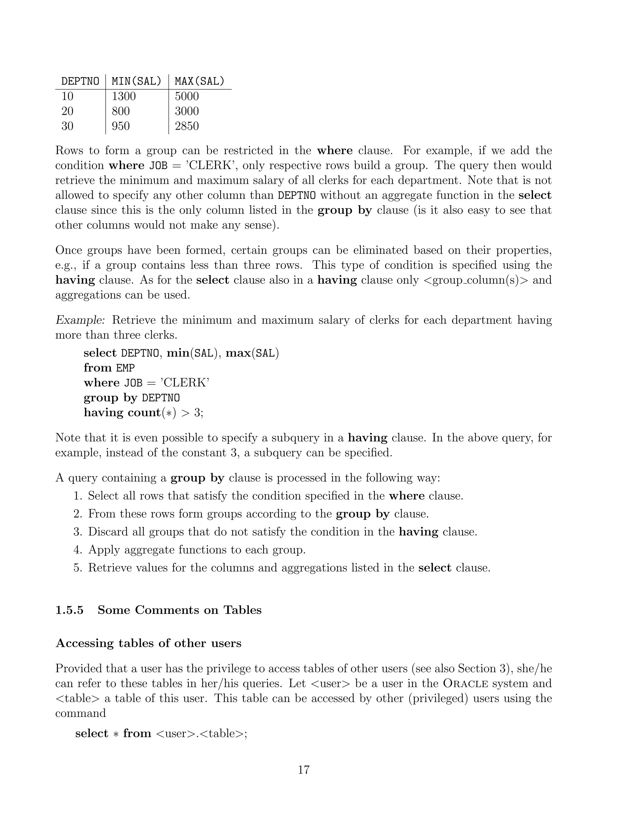
Example: For each department, we want to retrieve the minimum and maximum salary.
select DEPTNO, min(SAL), max(SAL)
from EMP
group by DEPTNO;
Rows from the table EMP are grouped such that all rows in a group have the same department
number. The aggregate functions are then applied to each such group. We thus get the following
query result:
16](https://image.slidesharecdn.com/cfakepathkunalboss-226-1b02c961-9cd4-4a44-ae8a-48f5f1c614ab-091113025135-phpapp01/75/SQL-18-2048.jpg)
![In case that one often refers to tables of other users, it is useful to use a synonym instead of
user.table. In Oracle-SQL a synonym can be created using the command
create synonym name for user.table ;
It is then possible to use simply name in a from clause. Synonyms can also be created for
one’s own tables.
Adding Comments to Definitions
For applications that include numerous tables, it is useful to add comments on table definitions
or to add comments on columns. A comment on a table can be created using the command
comment on table table is ’text’;
A comment on a column can be created using the command
comment on column table.column is ’text’;
Comments on tables and columns are stored in the data dictionary. They can be accessed using
the data dictionary views USER TAB COMMENTS and USER COL COMMENTS (see also Section 3).
Modifying Table- and Column Definitions
It is possible to modify the structure of a table (the relation schema) even if rows have already
been inserted into this table. A column can be added using the alter table command
alter table table
add(column data type [default value] [column constraint]);
If more than only one column should be added at one time, respective add clauses need to be
separated by colons. A table constraint can be added to a table using
alter table table add (table constraint);
Note that a column constraint is a table constraint, too. not null and primary key constraints
can only be added to a table if none of the specified columns contains a null value. Table
definitions can be modified in an analogous way. This is useful, e.g., when the size of strings
that can be stored needs to be increased. The syntax of the command for modifying a column
is
alter table table
modify(column [data type] [default value] [column constraint]);
Note: In earlier versions of Oracle it is not possible to delete single columns from a table
definition. A workaround is to create a temporary table and to copy respective columns and
rows into this new table. Furthermore, it is not possible to rename tables or columns. In the
most recent version (9i), using the alter table command, it is possible to rename a table,
columns, and constraints. In this version, there also exists a drop column clause as part of
the alter table statement.
Deleting a Table
A table and its rows can be deleted by issuing the command drop table table [cascade
constraints];.
18](https://image.slidesharecdn.com/cfakepathkunalboss-226-1b02c961-9cd4-4a44-ae8a-48f5f1c614ab-091113025135-phpapp01/75/SQL-20-2048.jpg)
![1.6 Views
In Oracle the SQL command to create a view (virtual table) has the form
create [or replace] view view-name [(column(s))] as
select-statement [with check option [constraint name]];
The optional clause or replace re-creates the view if it already exists. column(s) names
the columns of the view. If column(s) is not specified in the view definition, the columns of
the view get the same names as the attributes listed in the select statement (if possible).
Example: The following view contains the name, job title and the annual salary of em-
ployees working in the department 20:
create view DEPT20 as
select ENAME, JOB, SAL∗12 ANNUAL SALARY from EMP
where DEPTNO = 20;
In the select statement the column alias ANNUAL SALARY is specified for the expression SAL∗12
and this alias is taken by the view. An alternative formulation of the above view definition is
create view DEPT20 (ENAME, JOB, ANNUAL SALARY) as
select ENAME, JOB, SAL ∗ 12 from EMP
where DEPTNO = 20;
A view can be used in the same way as a table, that is, rows can be retrieved from a view
(also respective rows are not physically stored, but derived on basis of the select statement in
the view definition), or rows can even be modified. A view is evaluated again each time it is
accessed. In Oracle SQL no insert, update, or delete modifications on views are allowed
that use one of the following constructs in the view definition:
• Joins
• Aggregate function such as sum, min, max etc.
• set-valued subqueries (in, any, all) or test for existence (exists)
• group by clause or distinct clause
In combination with the clause with check option any update or insertion of a row into the
view is rejected if the new/modified row does not meet the view definition, i.e., these rows
would not be selected based on the select statement. A with check option can be named
using the constraint clause.
A view can be deleted using the command delete view-name.
19](https://image.slidesharecdn.com/cfakepathkunalboss-226-1b02c961-9cd4-4a44-ae8a-48f5f1c614ab-091113025135-phpapp01/75/SQL-21-2048.jpg)
![SQL is the prompt you get when you are connected to the Oracle database system. In
SQL*Plus you can divide a statement into separate lines, each continuing line is indicated by
a prompt such 2, 3 etc. An SQL statement must always be terminated by a semicolon (;).
In addition to the SQL statements discussed in the previous section, SQL*Plus provides some
special SQL*Plus commands. These commands need not be terminated by a semicolon. Upper
and lower case letters are only important for string comparisons. An SQL query can always be
interrupted by using ControlC. To exit SQL*Plus you can either type exit or quit.
Editor Commands
The most recently issued SQL statement is stored in the SQL buffer, independent of whether the
statement has a correct syntax or not. You can edit the buffer using the following commands:
• l[ist] lists all lines in the SQL buffer and sets the current line (marked with an ”∗”) to
the last line in the buffer.
• lnumber sets the actual line to number
• c[hange]/old string/new string replaces the first occurrence of old string by
new string (for the actual line)
• a[ppend]string appends string to the current line
• del deletes the current line
• r[un] executes the current buffer contents
• getfile reads the data from the file file into the buffer
• savefile writes the current buffer into the file file
• edit invokes an editor and loads the current buffer into the editor. After exiting the
editor the modified SQL statement is stored in the buffer and can be executed (command
r).
The editor can be defined in the SQL*Plus shell by typing the command define editor =
name, where name can be any editor such as emacs, vi, joe, or jove.
SQL*Plus Help System and Other Useful Commands
• To get the online help in SQL*Plus just type help command, or just help to get
information about how to use the help command. In Oracle Version 7 one can get the
complete list of possible commands by typing help command.
• To change the password, in Oracle Version 7 the command
alter user user identified by new password;
is used. In Oracle Version 8 the command passw user prompts the user for the
old/new password.
• The command desc[ribe] table lists all columns of the given table together with their
data types and information about whether null values are allowed or not.
• You can invoke a UNIX command from the SQL*Plus shell by using host UNIX command.
For example, host ls -la *.sql lists all SQL files in the current directory.
21](https://image.slidesharecdn.com/cfakepathkunalboss-226-1b02c961-9cd4-4a44-ae8a-48f5f1c614ab-091113025135-phpapp01/75/SQL-23-2048.jpg)
![• You can log your SQL*Plus session and thus queries and query results by using the
command spool file. All information displayed on screen is then stored in file
which automatically gets the extension .lst. The command spool off turns spooling off.
• The command copy can be used to copy a complete table. For example, the command
copy from scott/tiger create EMPL using select ∗ from EMP;
copies the table EMP of the user scott with password tiger into the relation EMPL. The
relation EMP is automatically created and its structure is derived based on the attributes
listed in the select clause.
• SQL commands saved in a file name.sql can be loaded into SQL*Plus and executed
using the command @name.
• Comments are introduced by the clause rem[ark] (only allowed between SQL statements),
or - - (allowed within SQL statements).
Formatting the Output
SQL*Plus provides numerous commands to format query results and to build simple reports.
For this, format variables are set and these settings are only valid during the SQL*Plus session.
They get lost after terminating SQL*Plus. It is, however, possible to save settings in a file named
login.sql in your home directory. Each time you invoke SQL*Plus this file is automatically
loaded.
The command column column name option 1 option 2 . . . is used to format columns
of your query result. The most frequently used options are:
• format An For alphanumeric data, this option sets the length of column name to
n. For columns having the data type number, the format command can be used to
specify the format before and after the decimal point. For example, format 99,999.99
specifies that if a value has more than three digits in front of the decimal point, digits are
separated by a colon, and only two digits are displayed after the decimal point.
• The option heading text relabels column name and gives it a new heading.
• null text is used to specify the output of null values (typically, null values are not
displayed).
• column column name clear deletes the format definitions for column name.
The command set linesize number can be used to set the maximum length of a single
line that can be displayed on screen. set pagesize number sets the total number of lines
SQL*Plus displays before printing the column names and headings, respectively, of the selected
rows.
Several other formatting features can be enabled by setting SQL*Plus variables. The command
show all displays all variables and their current values. To set a variable, type set variable
value. For example, set timing on causes SQL*Plus to display timing statistics for each
SQL command that is executed. set pause on [text] makes SQL*Plus wait for you to press
Return after the number of lines defined by set pagesize has been displayed. text is the
message SQL*Plus will display at the bottom of the screen as it waits for you to hit Return.
22](https://image.slidesharecdn.com/cfakepathkunalboss-226-1b02c961-9cd4-4a44-ae8a-48f5f1c614ab-091113025135-phpapp01/75/SQL-24-2048.jpg)
![3 Oracle Data Dictionary
The Oracle data dictionary is one of the most important components of the Oracle DBMS.
It contains all information about the structures and objects of the database such as tables,
columns, users, data files etc. The data stored in the data dictionary are also often called
metadata. Although it is usually the domain of database administrators (DBAs), the data
dictionary is a valuable source of information for end users and developers. The data dictionary
consists of two levels: the internal level contains all base tables that are used by the various
DBMS software components and they are normally not accessible by end users. The external
level provides numerous views on these base tables to access information about objects and
structures at different levels of detail.
3.1 Data Dictionary Tables
An installation of an Oracle database always includes the creation of three standard Oracle
users:
• SYS: This is the owner of all data dictionary tables and views. This user has the highest
privileges to manage objects and structures of an Oracle database such as creating new
users.
• SYSTEM: is the owner of tables used by different tools such SQL*Forms, SQL*Reports etc.
This user has less privileges than SYS.
• PUBLIC: This is a “dummy” user in an Oracle database. All privileges assigned to this
user are automatically assigned to all users known in the database.
The tables and views provided by the data dictionary contain information about
• users and their privileges,
• tables, table columns and their data types, integrity constraints, indexes,
• statistics about tables and indexes used by the optimizer,
• privileges granted on database objects,
• storage structures of the database.
The SQL command
select ∗ from DICT[IONARY];
lists all tables and views of the data dictionary that are accessible to the user. The selected
information includes the name and a short description of each table and view. Before issuing
this query, check the column definitions of DICT[IONARY] using desc DICT[IONARY] and set
the appropriate values for column using the format command.
The query
select ∗ from TAB;
retrieves the names of all tables owned by the user who issues this command. The query
select ∗ from COL;
23](https://image.slidesharecdn.com/cfakepathkunalboss-226-1b02c961-9cd4-4a44-ae8a-48f5f1c614ab-091113025135-phpapp01/75/SQL-25-2048.jpg)
![4.1.2 Structure of PL/SQL-Blocks
PL/SQL is a block-structured language. Each block builds a (named) program unit, and
blocks can be nested. Blocks that build a procedure, a function, or a package must be named.
A PL/SQL block has an optional declare section, a part containing PL/SQL statements, and an
optional exception-handling part. Thus the structure of a PL/SQL looks as follows (brackets
[ ] enclose optional parts):
[Block header]
[declare
Constants
Variables
Cursors
User defined exceptions]
begin
PL/SQL statements
[exception
Exception handling]
end;
The block header specifies whether the PL/SQL block is a procedure, a function, or a package.
If no header is specified, the block is said to be an anonymous PL/SQL block. Each PL/SQL
block again builds a PL/SQL statement. Thus blocks can be nested like blocks in conventional
programming languages. The scope of declared variables (i.e., the part of the program in which
one can refer to the variable) is analogous to the scope of variables in programming languages
such as C or Pascal.
4.1.3 Declarations
Constants, variables, cursors, and exceptions used in a PL/SQL block must be declared in the
declare section of that block. Variables and constants can be declared as follows:
variable name [constant] data type [not null] [:= expression];
Valid data types are SQL data types (see Section 1.1) and the data type boolean. Boolean
data may only be true, false, or null. The not null clause requires that the declared variable
must always have a value different from null. expression is used to initialize a variable.
If no expression is specified, the value null is assigned to the variable. The clause constant
states that once a value has been assigned to the variable, the value cannot be changed (thus
the variable becomes a constant). Example:
declare
hire date date; /* implicit initialization with null */
job title varchar2(80) := ’Salesman’;
emp found boolean; /* implicit initialization with null */
salary incr constant number(3,2) := 1.5; /* constant */
...
begin . . . end;
27](https://image.slidesharecdn.com/cfakepathkunalboss-226-1b02c961-9cd4-4a44-ae8a-48f5f1c614ab-091113025135-phpapp01/75/SQL-29-2048.jpg)
![Instead of specifying a data type, one can also refer to the data type of a table column (so-called
anchored declaration). For example, EMP.Empno%TYPE refers to the data type of the column
Empno in the relation EMP. Instead of a single variable, a record can be declared that can store a
complete tuple from a given table (or query result). For example, the data type DEPT%ROWTYPE
specifies a record suitable to store all attribute values of a complete row from the table DEPT.
Such records are typically used in combination with a cursor. A field in a record can be accessed
using record name.column name, for example, DEPT.Deptno.
A cursor declaration specifies a set of tuples (as a query result) such that the tuples can be
processed in a tuple-oriented way (i.e., one tuple at a time) using the fetch statement. A cursor
declaration has the form
cursor cursor name [(list of parameters)] is select statement;
The cursor name is an undeclared identifier, not the name of any PL/SQL variable. A parameter
has the form parameter name parameter type. Possible parameter types are char,
varchar2, number, date and boolean as well as corresponding subtypes such as integer.
Parameters are used to assign values to the variables that are given in the select statement.
Example: We want to retrieve the following attribute values from the table EMP in a tuple-
oriented way: the job title and name of those employees who have been hired
after a given date, and who have a manager working in a given department.
cursor employee cur (start date date, dno number) is
select JOB, ENAME from EMP E where HIREDATE start date
and exists (select ∗ from EMP
where E.MGR = EMPNO and DEPTNO = dno);
If (some) tuples selected by the cursor will be modified in the PL/SQL block, the clause for
update[(column(s))] has to be added at the end of the cursor declaration. In this case
selected tuples are locked and cannot be accessed by other users until a commit has been
issued. Before a declared cursor can be used in PL/SQL statements, the cursor must be
opened, and after processing the selected tuples the cursor must be closed. We discuss the
usage of cursors in more detail below.
Exceptions are used to process errors and warnings that occur during the execution of PL/SQL
statements in a controlled manner. Some exceptions are internally defined, such as ZERO DIVIDE.
Other exceptions can be specified by the user at the end of a PL/SQL block. User defined ex-
ceptions need to be declared using name of exception exception. We will discuss exception
handling in more detail in Section 4.1.5
4.1.4 Language Elements
In addition to the declaration of variables, constants, and cursors, PL/SQL offers various lan-
guage constructs such as variable assignments, control structures (loops, if-then-else), procedure
and function calls, etc. However, PL/SQL does not allow commands of the SQL data definition
language such as the create table statement. For this, PL/SQL provides special packages.
28](https://image.slidesharecdn.com/cfakepathkunalboss-226-1b02c961-9cd4-4a44-ae8a-48f5f1c614ab-091113025135-phpapp01/75/SQL-30-2048.jpg)
![Furthermore, PL/SQL uses a modified select statement that requires each selected tuple to be
assigned to a record (or a list of variables).
There are several alternatives in PL/SQL to a assign a value to a variable. The most simple
way to assign a value to a variable is
declare
counter integer := 0;
...
begin
counter := counter + 1;
Values to assign to a variable can also be retrieved from the database using a select statement
select column(s) into matching list of variables
from table(s) where condition;
It is important to ensure that the select statement retrieves at most one tuple ! Otherwise
it is not possible to assign the attribute values to the specified list of variables and a run-
time error occurs. If the select statement retrieves more than one tuple, a cursor must be used
instead. Furthermore, the data types of the specified variables must match those of the retrieved
attribute values. For most data types, PL/SQL performs an automatic type conversion (e.g.,
from integer to real).
Instead of a list of single variables, a record can be given after the keyword into. Also in this
case, the select statement must retrieve at most one tuple !
declare
employee rec EMP%ROWTYPE;
max sal EMP.SAL%TYPE;
begin
select EMPNO, ENAME, JOB, MGR, SAL, COMM, HIREDATE, DEPTNO
into employee rec
from EMP where EMPNO = 5698;
select max(SAL) into max sal from EMP;
...
end;
PL/SQL provides while-loops, two types of for-loops, and continuous loops. Latter ones
are used in combination with cursors. All types of loops are used to execute a sequence of
statements multiple times. The specification of loops occurs in the same way as known from
imperative programming languages such as C or Pascal.
A while-loop has the pattern
[ label name ]
while condition loop
sequence of statements;
end loop [label name] ;
29](https://image.slidesharecdn.com/cfakepathkunalboss-226-1b02c961-9cd4-4a44-ae8a-48f5f1c614ab-091113025135-phpapp01/75/SQL-31-2048.jpg)
![A loop can be named. Naming a loop is useful whenever loops are nested and inner loops are
completed unconditionally using the exit label name; statement.
Whereas the number of iterations through a while loop is unknown until the loop completes,
the number of iterations through the for loop can be specified using two integers.
[ label name ]
for index in [reverse] lower bound..upper bound loop
sequence of statements
end loop [label name] ;
The loop counter index is declared implicitly. The scope of the loop counter is only the
for loop. It overrides the scope of any variable having the same name outside the loop. Inside
the for loop, index can be referenced like a constant. index may appear in expressions,
but one cannot assign a value to index. Using the keyword reverse causes the iteration to
proceed downwards from the higher bound to the lower bound.
Processing Cursors: Before a cursor can be used, it must be opened using the open statement
open cursor name [(list of parameters)] ;
The associated select statement then is processed and the cursor references the first selected
tuple. Selected tuples then can be processed one tuple at a time using the fetch command
fetch cursor name into list of variables;
The fetch command assigns the selected attribute values of the current tuple to the list of
variables. After the fetch command, the cursor advances to the next tuple in the result set.
Note that the variables in the list must have the same data types as the selected values. After
all tuples have been processed, the close command is used to disable the cursor.
close cursor name;
The example below illustrates how a cursor is used together with a continuous loop:
declare
cursor emp cur is select ∗ from EMP;
emp rec EMP%ROWTYPE;
emp sal EMP.SAL%TYPE;
begin
open emp cur;
loop
fetch emp cur into emp rec;
exit when emp cur%NOTFOUND;
emp sal := emp rec.sal;
sequence of statements
end loop;
close emp cur;
...
end;
30](https://image.slidesharecdn.com/cfakepathkunalboss-226-1b02c961-9cd4-4a44-ae8a-48f5f1c614ab-091113025135-phpapp01/75/SQL-32-2048.jpg)
![Each loop can be completed unconditionally using the exit clause:
exit [block label] [when condition]
Using exit without a block label causes the completion of the loop that contains the exit state-
ment. A condition can be a simple comparison of values. In most cases, however, the condition
refers to a cursor. In the example above, %NOTFOUND is a predicate that evaluates to false if the
most recent fetch command has read a tuple. The value of cursor name%NOTFOUND is null
before the first tuple is fetched. The predicate evaluates to true if the most recent fetch failed
to return a tuple, and false otherwise. %FOUND is the logical opposite of %NOTFOUND.
Cursor for loops can be used to simplify the usage of a cursor:
[ label name ]
for record name in cursor name[(list of parameters)] loop
sequence of statements
end loop [label name];
A record suitable to store a tuple fetched by the cursor is implicitly declared. Furthermore,
this loop implicitly performs a fetch at each iteration as well as an open before the loop is
entered and a close after the loop is left. If at an iteration no tuple has been fetched, the loop
is automatically terminated without an exit.
It is even possible to specify a query instead of cursor name in a for loop:
for record name in (select statement) loop
sequence of statements
end loop;
That is, a cursor needs not be specified before the loop is entered, but is defined in the select
statement.
Example:
for sal rec in (select SAL + COMM total from EMP) loop
...;
end loop;
total is an alias for the expression computed in the select statement. Thus, at each iteration
only one tuple is fetched. The record sal rec, which is implicitly defined, then contains only
one entry which can be accessed using sal rec.total. Aliases, of course, are not necessary if
only attributes are selected, that is, if the select statement contains no arithmetic operators
or aggregate functions.
For conditional control, PL/SQL offers if-then-else constructs of the pattern
if condition then sequence of statements
[elsif ] condition then sequence of statements
...
[else] sequence of statements end if ;
31](https://image.slidesharecdn.com/cfakepathkunalboss-226-1b02c961-9cd4-4a44-ae8a-48f5f1c614ab-091113025135-phpapp01/75/SQL-33-2048.jpg)
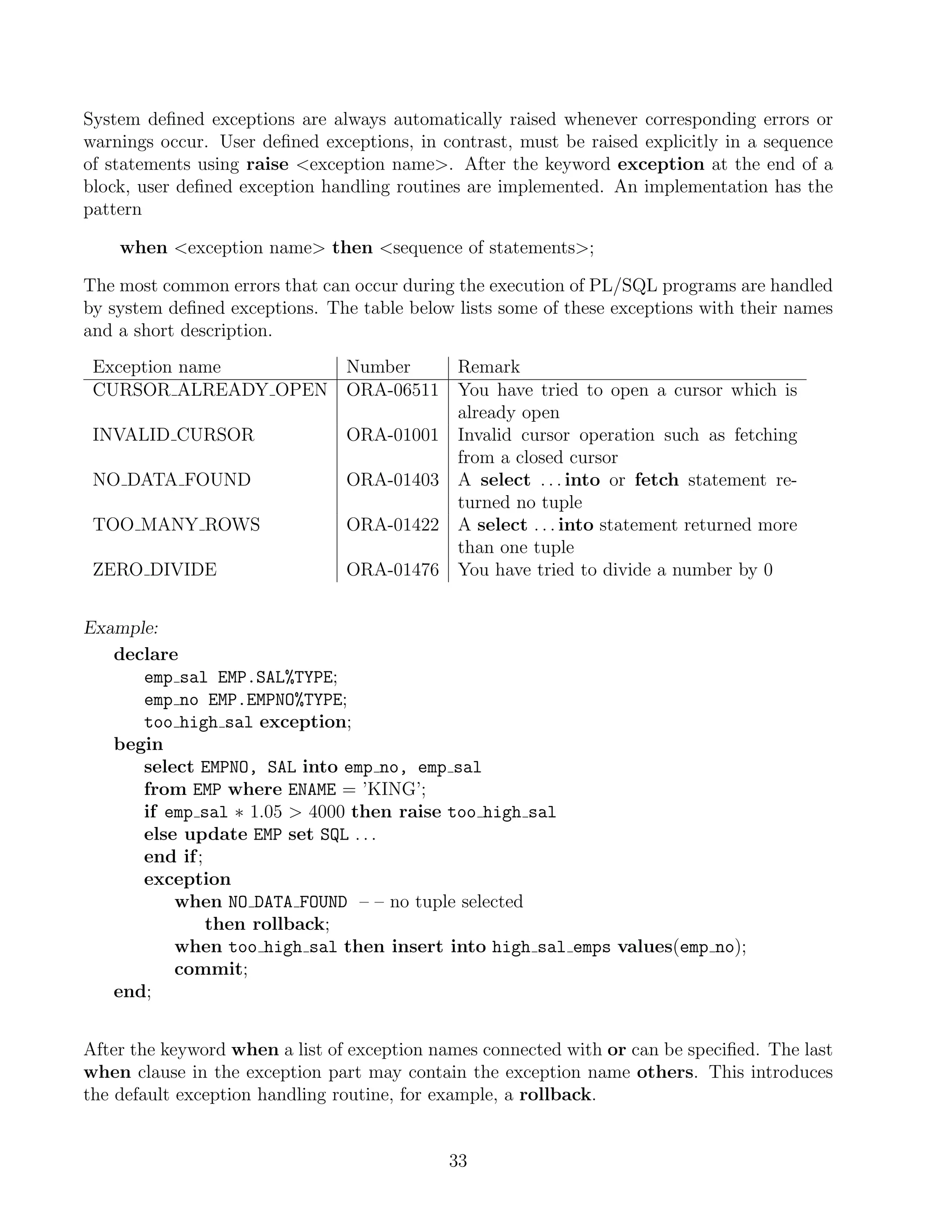
![If a PL/SQL program is executed from the SQL*Plus shell, exception handling routines may
contain statements that display error or warning messages on the screen. For this, the procedure
raise application error can be used. This procedure has two parameters error number
and message text. error number is a negative integer defined by the user and must range
between -20000 and -20999. error message is a string with a length up to 2048 characters.
The concatenation operator “||” can be used to concatenate single strings to one string. In order
to display numeric variables, these variables must be converted to strings using the function
to char. If the procedure raise application error is called from a PL/SQL block, processing
the PL/SQL block terminates and all database modifications are undone, that is, an implicit
rollback is performed in addition to displaying the error message.
Example:
if emp sal ∗ 1.05 4000
then raise application error(-20010, ’Salary increase for employee with Id ’
|| to char(Emp no) || ’ is too high’);
4.1.6 Procedures and Functions
PL/SQL provides sophisticated language constructs to program procedures and functions as
stand-alone PL/SQL blocks. They can be called from other PL/SQL blocks, other procedures
and functions. The syntax for a procedure definition is
create [or replace] procedure procedure name [(list of parameters)] is
declarations
begin
sequence of statements
[exception
exception handling routines]
end [procedure name];
A function can be specified in an analogous way
create [or replace] function function name [(list of parameters)]
return data type is
...
The optional clause or replace re-creates the procedure/function. A procedure can be deleted
using the command drop procedure procedure name (drop function function name).
In contrast to anonymous PL/SQL blocks, the clause declare may not be used in proce-
dure/function definitions.
Valid parameters include all data types. However, for char, varchar2, and number no length
and scale, respectively, can be specified. For example, the parameter number(6) results in a
compile error and must be replaced by number. Instead of explicit data types, implicit types
of the form %TYPE and %ROWTYPE can be used even if constrained declarations are referenced.
A parameter is specified as follows:
parameter name [IN | OUT | IN OUT] data type [{ := | DEFAULT} expression]
34](https://image.slidesharecdn.com/cfakepathkunalboss-226-1b02c961-9cd4-4a44-ae8a-48f5f1c614ab-091113025135-phpapp01/75/SQL-36-2048.jpg)
![all sal := all sal + emp sal.sal;
end loop;
return all sal;
end get dept salary;
In order to call a function from the SQL*Plus shell, it is necessary to first define a vari-
able to which the return value can be assigned. In SQL*Plus a variable can be defined us-
ing the command variable variable name data type;, for example, variable salary
number. The above function then can be called using the command execute :salary :=
get dept salary(20); Note that the colon “:” must be put in front of the variable.
Further information about procedures and functions can be obtained using the help command
in the SQL*Plus shell, for example, help [create] function, help subprograms, help stored
subprograms.
4.1.7 Packages
It is essential for a good programming style that logically related blocks, procedures, and func-
tions are combined into modules, and each module provides an interface which allows users
and designers to utilize the implemented functionality. PL/SQL supports the concept of mod-
ularization by which modules and other constructs can be organized into packages. A package
consists of a package specification and a package body. The package specification defines the
interface that is visible for application programmers, and the package body implements the
package specification (similar to header- and source files in the programming language C).
Below a package is given that is used to combine all functions and procedures to manage
information about employees.
create package manage_employee as -- package specification
function hire_emp (name varchar2, job varchar2, mgr number, hiredate date,
sal number, comm number default 0, deptno number)
return number;
procedure fire_emp (emp_id number);
procedure raise_sal (emp_id number, sal_incr number);
end manage_employee;
create package body manage_employee as
function hire_emp (name varchar2, job varchar2, mgr number, hiredate date,
sal number, comm number default 0, deptno number)
return number is
-- Insert a new employee with a new employee Id
new_empno number(10);
begin
select emp_sequence.nextval into new_empno from dual;
36](https://image.slidesharecdn.com/cfakepathkunalboss-226-1b02c961-9cd4-4a44-ae8a-48f5f1c614ab-091113025135-phpapp01/75/SQL-38-2048.jpg)
![insert into emp values(new_empno, name, job, mgr, hiredate,
sal, comm, deptno);
return new_empno;
end hire_emp;
procedure fire_emp(emp_id number) is
-- deletes an employee from the table EMP
begin
delete from emp where empno = emp_id;
if SQL%NOTFOUND then -- delete statement referred to invalid emp_id
raise_application_error(-20011, ’Employee with Id ’ ||
to_char(emp_id) || ’ does not exist.’);
end if;
end fire_emp;
procedure raise_sal(emp_id number, sal_incr number) is
-- modify the salary of a given employee
begin
update emp set sal = sal + sal_incr
where empno = emp_id;
if SQL%NOTFOUND then
raise_application_error(-20012, ’Employee with Id ’ ||
to_char(emp_id) || ’ does not exist’);
end if;
end raise_sal;
end manage_employee;
Remark: In order to compile and execute the above package, it is necessary to create first the
required sequence (help sequence):
create sequence emp sequence start with 8000 increment by 10;
A procedure or function implemented in a package can be called from other procedures and
functions using the statement package name.procedure name[(list of parameters)].
Calling such a procedure from the SQL*Plus shell requires a leading execute.
Oracle offers several predefined packages and procedures that can be used by database users
and application developers. A set of very useful procedures is implemented in the package
DBMS OUTPUT. This package allows users to display information to their SQL*Plus session’s
screen as a PL/SQL program is executed. It is also a very useful means to debug PL/SQL
programs that have been successfully compiled, but do not behave as expected. Below some of
the most important procedures of this package are listed:
37](https://image.slidesharecdn.com/cfakepathkunalboss-226-1b02c961-9cd4-4a44-ae8a-48f5f1c614ab-091113025135-phpapp01/75/SQL-39-2048.jpg)
![Procedure name Remark
DBMS OUTPUT.ENABLE enables output
DBMS OUTPUT.DISABLE disables output
DBMS OUTPUT.PUT(string) appends (displays) string to output
buffer
DBMS OUTPUT.PUT LINE(string) appends string to output buffer and
appends a new-line marker
DBMS OUTPUT.NEW LINE displays a new-line marker
Before strings can be displayed on the screen, the output has to be enabled either using the
procedure DBMS OUTPUT.ENABLE or using the SQL*Plus command set serveroutput on (before
the procedure that produces the output is called).
Further packages provided by Oracle are UTL FILE for reading and writing files from PL/SQL
programs, DBMS JOB for job scheduling, and DBMS SQL to generate SQL statements dynamically,
that is, during program execution. The package DBMS SQL is typically used to create and
delete tables from within PL/SQL programs. More packages can be found in the directory
$ORACLE HOME/rdbms/admin.
4.1.8 Programming in PL/SQL
Typically one uses an editor such as emacs or vi to write a PL/SQL program. Once a program
has been stored in a file name with the extension .sql, it can be loaded into SQL*Plus
using the command @name. It is important that the last line of the file contains a slash
“/”.
If the procedure, function, or package has been successfully compiled, SQL*Plus displays the
message PL/SQL procedure successfully completed. If the program contains errors, these
are displayed in the format ORA-n message text, where n is a number and message text is
a short description of the error, for example, ORA-1001 INVALID CURSOR. The SQL*Plus com-
mand show errors [function|procedure|package|package body|trigger name] displays all
compilation errors of the most recently created or altered function (or procedure, or package
etc.) in more detail. If this command does not show any errors, try select ∗ from USER ERRORS.
Under the UNIX shell one can also use the command oerr ORA n to get information of the
following form:
error description
Cause: Reason for the error
Action: Suggested action
38](https://image.slidesharecdn.com/cfakepathkunalboss-226-1b02c961-9cd4-4a44-ae8a-48f5f1c614ab-091113025135-phpapp01/75/SQL-40-2048.jpg)
![Editor Program Development
Host Program including SQL and PL/SQL commands
Program (program.pc)
Precompiler Translates SQL and PL/SQL commands into function calls
Source ‘pure’ C−Program including libraries (.h)
Program (program.c)
C−Compiler cc, gcc or g++
Object− executable
Program Linker Program
Oracle Run−Time Library C Standard−Libraries
Figure 1: Translation of a Pro*C Program
char Name single character
char Name[n] array of n characters
int integer
float floating point
VARCHARName[n] variable length strings
VARCHAR2 is converted by the Pro*C precompiler into a structure with an n-byte character
array and a 2-bytes length field. The declaration of host variables occurs in a declare section
having the following pattern:
EXEC SQL BEGIN DECLARE SECTION
Declaration of host variables
/* e.g., VARCHAR userid[20]; */
/* e.g., char test ok; */
EXEC SQL END DECLARE SECTION
In a Pro*C program at most one such a declare section is allowed. The declaration of cursors
and exceptions occurs outside of such a declare section for host variables. In a Pro*C program
host variables referenced in SQL and PL/SQL statements must be prefixed with a colon “:”.
Note that it is not possible to use C function calls and most of the pointer expressions as host
variable references.
2
Note: all uppercase letters; varchar2 is not allowed!
40](https://image.slidesharecdn.com/cfakepathkunalboss-226-1b02c961-9cd4-4a44-ae8a-48f5f1c614ab-091113025135-phpapp01/75/SQL-42-2048.jpg)
![4.2.3 The Communication Area
In addition to host language variables that are needed to pass data between the database and
C program (and vice versa), one needs to provide some status variables containing program
runtime information. The variables are used to pass status information concerning the database
access to the application program so that certain events can be handled in the program properly.
The structure containing the status variables is called SQL Communication Area or SQLCA,
for short, and has to be included after the declare section using the statement
EXEC SQL INCLUDE SQLCA.H
In the variables defined in this structure, information about error messages as well as program
status information is maintained:
struct sqlca
{
/* ub1 */ char sqlcaid[8];
/* b4 */ long sqlabc;
/* b4 */ long sqlcode;
struct
{
/* ub2 */ unsigned short sqlerrml;
/* ub1 */ char sqlerrmc[70];
} sqlerrm;
/* ub1 */ char sqlerrp[8];
/* b4 */ long sqlerrd[6];
/* ub1 */ char sqlwarn[8];
/* ub1 */ char sqlext[8];
};
The fields in this structure have the following meaning:
sqlcaid Used to identify the SQLCA, set to “SQLCA”
sqlabc Holds the length of the SQLCA structure
sqlcode Holds the status code of the most recently executed SQL (PL/SQL) statement
0 = No error, statement successfully completed
ˆ
0 = Statement executed and exception detected. Typical situations are where
ˆ
fetch or select into returns no rows.
0 = Statement was not executed because of an error; transaction should
ˆ
be rolled back explicitly.
sqlerrm Structure with two components
sqlerrml: length of the message text in sqlerrmc, and
sqlerrmc: error message text (up to 70 characters) corresponding to the error
code recorded in sqlcode
sqlerrp Not used
41](https://image.slidesharecdn.com/cfakepathkunalboss-226-1b02c961-9cd4-4a44-ae8a-48f5f1c614ab-091113025135-phpapp01/75/SQL-43-2048.jpg)
![sqlerrd Array of binary integers, has 6 elements:
sqlerrd[0],sqlerrd[1],sqlerrd[3],sqlerrd[6] not used; sqlerrd[2] =
number of rows processed by the most recent SQL statement; sqlerrd[4] =
offset specifying position of most recent parse error of SQL statement.
sqlwarn Array with eight elements used as warning (not error!) flags. Flag is set by
assigning it the character ‘W’.
sqlwarn[0]: only set if other flag is set
sqlwarn[1]: if truncated column value was assigned to a host variable
sqlwarn[2]: null column is not used in computing an aggregate function
sqlwarn[3]: number of columns in select is not equal to number of host
variables specified in into
sqlwarn[4]: if every tuple was processed by an update or delete statement
without a where clause
sqlwarn[5]: procedure/function body compilation failed because of
a PL/SQL error
sqlwarn[6] and sqlwarn[7]: not used
sqlext not used
Components of this structure can be accessed and verified during runtime, and appropriate
handling routines (e.g., exception handling) can be executed to ensure a correct behavior of the
application program. If at the end of the program the variable sqlcode contains a 0, then the
execution of the program has been successful, otherwise an error occurred.
4.2.4 Exception Handling
There are two ways to check the status of your program after executable SQL statements which
may result in an error or warning: (1) either by explicitly checking respective components
of the SQLCA structure, or (2) by doing automatic error checking and handling using the
WHENEVER statement. The complete syntax of this statement is
EXEC SQL WHENEVER condition action;
By using this command, the program then automatically checks the SQLCA for condition
and executes the given action. condition can be one of the following:
• SQLERROR: sqlcode has a negative value, that is, an error occurred
• SQLWARNING: In this case sqlwarn[0] is set due to a warning
• NOT FOUND: sqlcode has a positive value, meaning that no row was found that satisfies
the where condition, or a select into or fetch statement returned no rows
action can be
• STOP: the program exits with an exit() call, and all SQL statements that have not
been committed so far are rolled back
42](https://image.slidesharecdn.com/cfakepathkunalboss-226-1b02c961-9cd4-4a44-ae8a-48f5f1c614ab-091113025135-phpapp01/75/SQL-44-2048.jpg)
![#include stdlib.h
/* Declare section for host variables */
EXEC SQL BEGIN DECLARE SECTION;
VARCHAR userid[20];
VARCHAR passwd[20];
int empno;
VARCHAR ename[15];
float sal;
float min_sal;
EXEC SQL END DECLARE SECTION;
/* Load SQL Communication Area */
EXEC SQL INCLUDE SQLCA.H;
main() /* Main program */
{ int retval;
/* Catch errors automatically and go to error handling rountine */
EXEC SQL WHENEVER SQLERROR GOTO error;
/* Connect to Oracle as SCOTT/TIGER; both are host variables */
/* of type VARCHAR; Account and Password are specified explicitly */
strcpy(userid.arr,SCOTT); /* userid.arr := SCOTT */
userid.len=strlen(userid.arr); /* uid.len := 5 */
strcpy(passwd.arr,SCOTT); /* passwd.arr := TIGER */
passwd.len=strlen(passwd.arr); /* passwd.len := 5 */
EXEC SQL CONNECT :userid IDENTIFIED BY :passwd;
printf(Connected to ORACLE as: %snn, userid.arr);
/* Enter minimum salary by user */
printf(Please enter minimum salary );
retval = scanf(%f, min_sal);
if(retval != 1) {
printf(Input error!!n);
EXEC SQL ROLLBACK WORK RELEASE;
/* Disconnect from ORACLE */
exit(2); /* Exit program */
}
/* Declare cursor; cannot occur in declare section! */
EXEC SQL DECLARE EMP_CUR CURSOR FOR
SELECT EMPNO,ENAME,SAL FROM EMP
44](https://image.slidesharecdn.com/cfakepathkunalboss-226-1b02c961-9cd4-4a44-ae8a-48f5f1c614ab-091113025135-phpapp01/75/SQL-46-2048.jpg)
![WHERE SAL=:min_sal;
/* Print Table header, run cursor through result set */
printf(Empployee-ID Employee-Name Salary n);
printf(--------------- ----------------- -------n);
EXEC SQL OPEN EMP_CUR;
EXEC SQL FETCH EMP_CUR INTO :empno, :ename, :sal; /* Fetch 1.tuple */
while(sqlca.sqlcode==0) { /* are there more tuples ? */
ename.arr[ename.len] = ’0’; /* End of String */
printf(%15d %-17s %7.2fn,empno,ename.arr,sal);
EXEC SQL FETCH EMP_CUR INTO :empno, :ename, :sal; /* get next tuple */
}
EXEC SQL CLOSE EMP_CUR;
/* Disconnect from database and terminate program */
EXEC SQL COMMIT WORK RELEASE;
printf(nDisconnected from ORACLEn);
exit(0);
/* Error Handling: Print error message */
error: printf(nError: %.70s n,sqlca.sqlerrm.sqlerrmc);
EXEC SQL ROLLBACK WORK RELEASE;
exit(1);
}
45](https://image.slidesharecdn.com/cfakepathkunalboss-226-1b02c961-9cd4-4a44-ae8a-48f5f1c614ab-091113025135-phpapp01/75/SQL-47-2048.jpg)
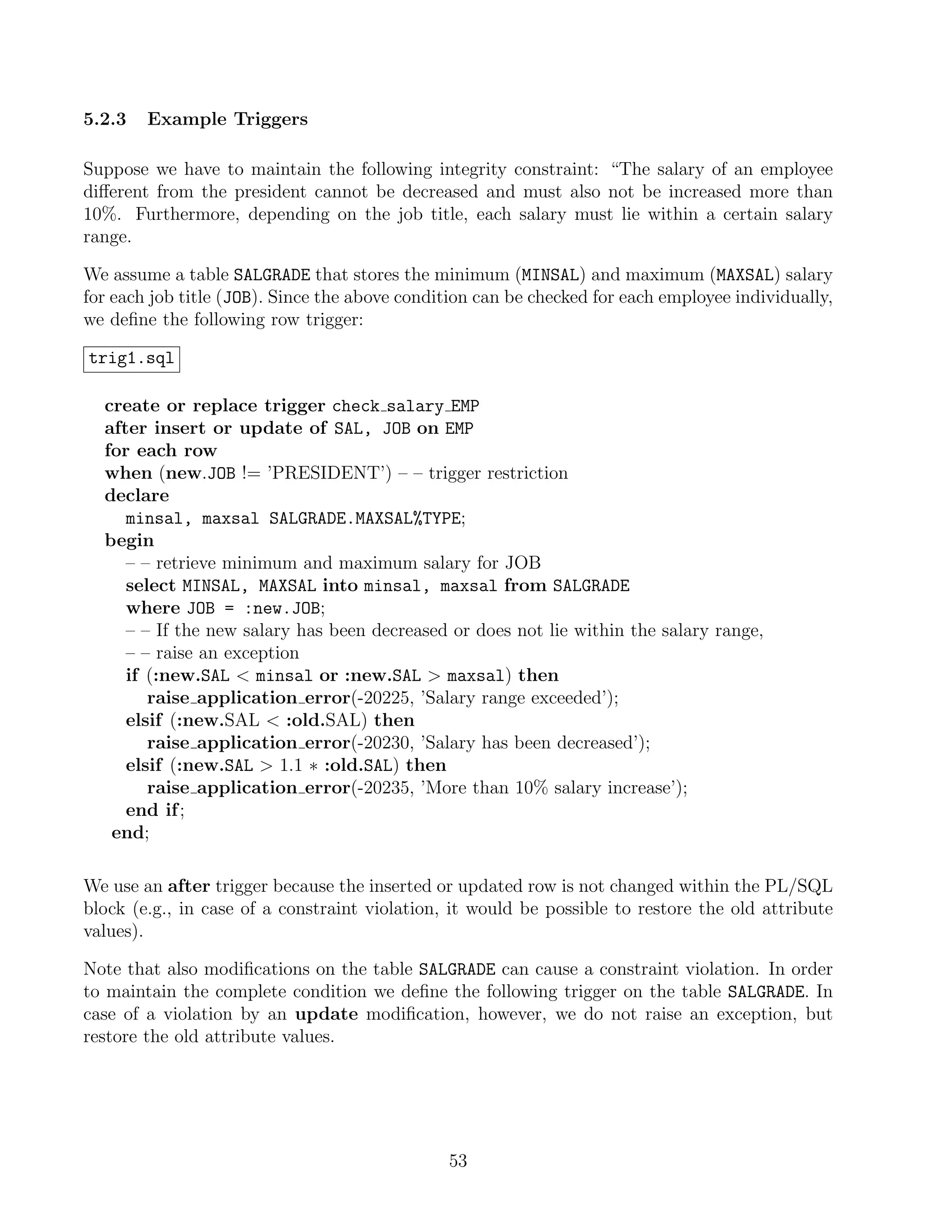
![5 Integrity Constraints and Triggers
5.1 Integrity Constraints
In Section 1 we have discussed three types of integrity constraints: not null constraints, primary
keys, and unique constraints. In this section we introduce two more types of constraints that
can be specified within the create table statement: check constraints (to restrict possible
attribute values), and foreign key constraints (to specify interdependencies between relations).
5.1.1 Check Constraints
Often columns in a table must have values that are within a certain range or that satisfy certain
conditions. Check constraints allow users to restrict possible attribute values for a column to
admissible ones. They can be specified as column constraints or table constraints. The syntax
for a check constraint is
[constraint name] check(condition)
If a check constraint is specified as a column constraint, the condition can only refer that
column.
Example: The name of an employee must consist of upper case letters only; the minimum
salary of an employee is 500; department numbers must range between 10 and
100:
create table EMP
( ...,
ENAME varchar2(30) constraint check name
check(ENAME = upper(ENAME) ),
SAL number(5,2) constraint check sal check(SAL = 500),
DEPTNO number(3) constraint check deptno
check(DEPTNO between 10 and 100) );
If a check constraint is specified as a table constraint, condition can refer to all columns
of the table. Note that only simple conditions are allowed. For example, it is not allowed
to refer to columns of other tables or to formulate queries as check conditions. Furthermore,
the functions sysdate and user cannot be used in a condition. In principle, thus only simple
attribute comparisons and logical connectives such as and, or, and not are allowed. A check
condition, however, can include a not null constraint:
SAL number(5,2) constraint check sal check(SAL is not null and SAL = 500),
Without the not null condition, the value null for the attribute SAL would not cause a violation
of the constraint.
Example: At least two persons must participate in a project, and the project’s start date
must be before the project’s end date:
46](https://image.slidesharecdn.com/cfakepathkunalboss-226-1b02c961-9cd4-4a44-ae8a-48f5f1c614ab-091113025135-phpapp01/75/SQL-48-2048.jpg)
![create table PROJECT
( ...,
PERSONS number(5) constraint check pers check (PERSONS 2),
...,
constraint dates ok check(PEND PSTART) );
In this table definition, check pers is a column constraint and dates ok is a table constraint.
The database system automatically checks the specified conditions each time a database mod-
ification is performed on this relation. For example, the insertion
insert into EMP values(7999,’SCOTT’,’CLERK’,7698,’31-OCT-94’,450,10);
causes a constraint violation
ORA-02290: check constraint (CHECK SAL) violated
and the insertion is rejected.
5.1.2 Foreign Key Constraints
A foreign key constraint (or referential integrity constraint) can be specified as a column con-
straint or as a table constraint:
[constraint name] [foreign key (column(s))]
references table[(column(s))]
[on delete cascade]
This constraint specifies a column or a list of columns as a foreign key of the referencing table.
The referencing table is called the child-table, and the referenced table is called the parent-table.
In other words, one cannot define a referential integrity constraint that refers to a table R before
that table R has been created.
The clause foreign key has to be used in addition to the clause references if the foreign
key includes more than one column. In this case, the constraint has to be specified as a table
constraint. The clause references defines which columns of the parent-table are referenced. If
only the name of the parent-table is given, the list of attributes that build the primary key of
that table is assumed.
Example: Each employee in the table EMP must work in a department that is contained
in the table DEPT:
create table EMP
( EMPNO number(4) constraint pk emp primary key,
...,
DEPTNO number(3) constraint fk deptno references DEPT(DEPTNO) );
The column DEPTNO of the table EMP (child-table) builds the foreign key and references the
primary key of the table DEPT (parent-table). The relationship between these two tables is
illustrated in Figure 2. Since in this table definition the referential integrity constraint includes
47](https://image.slidesharecdn.com/cfakepathkunalboss-226-1b02c961-9cd4-4a44-ae8a-48f5f1c614ab-091113025135-phpapp01/75/SQL-49-2048.jpg)
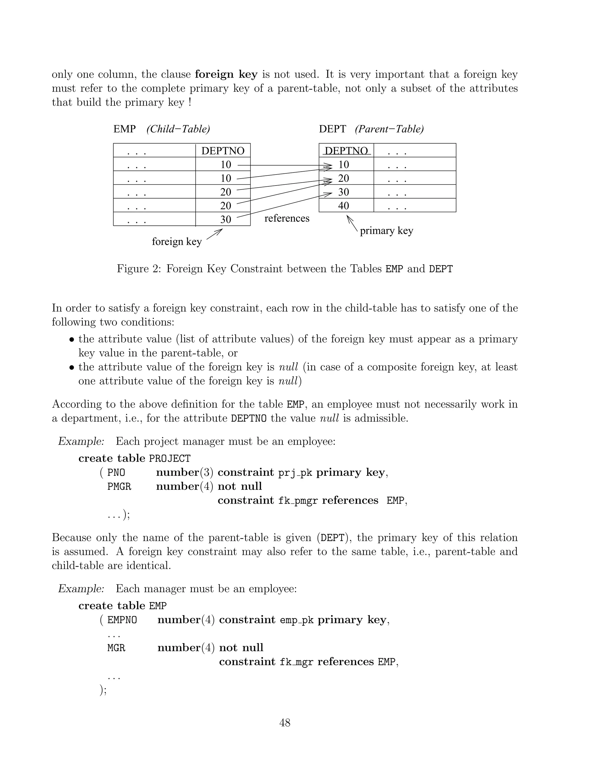
![5.1.3 More about Column- and Table Constraints
If a constraint is defined within the create table command or added using the alter table
command (compare Section 1.5.5), the constraint is automatically enabled. A constraint can
be disabled using the command
alter table table disable
constraint name | primary key | unique[column(s)]
[cascade];
To disable a primary key, one must disable all foreign key constraints that depend on this
primary key. The clause cascade automatically disables foreign key constraints that depend
on the (disabled) primary key.
Example: Disable the primary key of the table DEPT and disable the foreign key constraint
in the table EMP:
alter table DEPT disable primary key cascade;
In order to enable an integrity constraint, the clause enable is used instead of disable. A
constraint can only be enabled successfully if no tuple in the table violates the constraint. Oth-
erwise an error message is displayed. Note that for enabling/disabling an integrity constraint
it is important that you have named the constraints.
In order to identify those tuples that violate an integrity constraint whose activation failed, one
can use the clause exceptions into EXCEPTIONS with the alter table statement. EXCEPTIONS
is a table that stores information about violating tuples.3 Each tuple in this table is identified
by the attribute ROWID. Every tuple in a database has a pseudo-column ROWID that is used to
identify tuples. Besides the rowid, the name of the table, the table owner as well as the name
of the violated constraint are stored.
Example: Assume we want to add an integrity constraint to our table EMP which requires
that each manager must earn more than 4000:
alter table EMP add constraint manager sal
check(JOB != ’MANAGER’ or SAL = 4000)
exceptions into EXCEPTIONS;
If the table EMP already contains tuples that violate the constraint, the constraint cannot
be activated and information about violating tuples is automatically inserted into the table
EXCEPTIONS.
Detailed information about the violating tuples can be obtained by joining the tables EMP and
EXCEPTIONS, based on the join attribute ROWID:
select EMP.∗, CONSTRAINT from EMP, EXCEPTIONS
where EMP.ROWID = EXCEPTIONS.ROW ID;
3
Before this table can be used, it must be created using the SQL script utlexcept.sql which can be found
in the directory $ORACLE HOME/rdbms/admin.
49](https://image.slidesharecdn.com/cfakepathkunalboss-226-1b02c961-9cd4-4a44-ae8a-48f5f1c614ab-091113025135-phpapp01/75/SQL-51-2048.jpg)
![Tuples contained in the query result now can be modified (e.g., by increasing the salary of
managers) such that adding the constraint can be performed successfully. Note that it is
important to delete “old” violations from the relation EXCEPTIONS before it is used again.
If a table is used as a reference of a foreign key, this table can only be dropped using the
command drop table table cascade constraints;. All other database objects that refer
to this table (e.g., triggers, see Section 5.2) remain in the database system, but they are not
valid.
Information about integrity constraints, their status (enabled, disabled) etc. is stored in the
data dictionary, more precisely, in the tables USER CONSTRAINTS and USER CONS CONSTRAINTS.
5.2 Triggers
5.2.1 Overview
The different types of integrity constraints discussed so far provide a declarative mechanism
to associate “simple” conditions with a table such as a primary key, foreign keys or domain
constraints. Complex integrity constraints that refer to several tables and attributes (as they
are known as assertions in the SQL standard) cannot be specified within table definitions. Trig-
gers, in contrast, provide a procedural technique to specify and maintain integrity constraints.
Triggers even allow users to specify more complex integrity constraints since a trigger essen-
tially is a PL/SQL procedure. Such a procedure is associated with a table and is automatically
called by the database system whenever a certain modification (event) occurs on that table.
Modifications on a table may include insert, update, and delete operations (Oracle 7).
5.2.2 Structure of Triggers
A trigger definition consists of the following (optional) components:
• trigger name
create [or replace] trigger trigger name
• trigger time point
before | after
• triggering event(s)
insert or update [of column(s)] or delete on table
• trigger type (optional)
for each row
• trigger restriction (only for for each row triggers !)
when (condition)
• trigger body
PL/SQL block
The clause replace re-creates a previous trigger definition having the same trigger name.
The name of a trigger can be chosen arbitrarily, but it is a good programming style to use
50](https://image.slidesharecdn.com/cfakepathkunalboss-226-1b02c961-9cd4-4a44-ae8a-48f5f1c614ab-091113025135-phpapp01/75/SQL-52-2048.jpg)
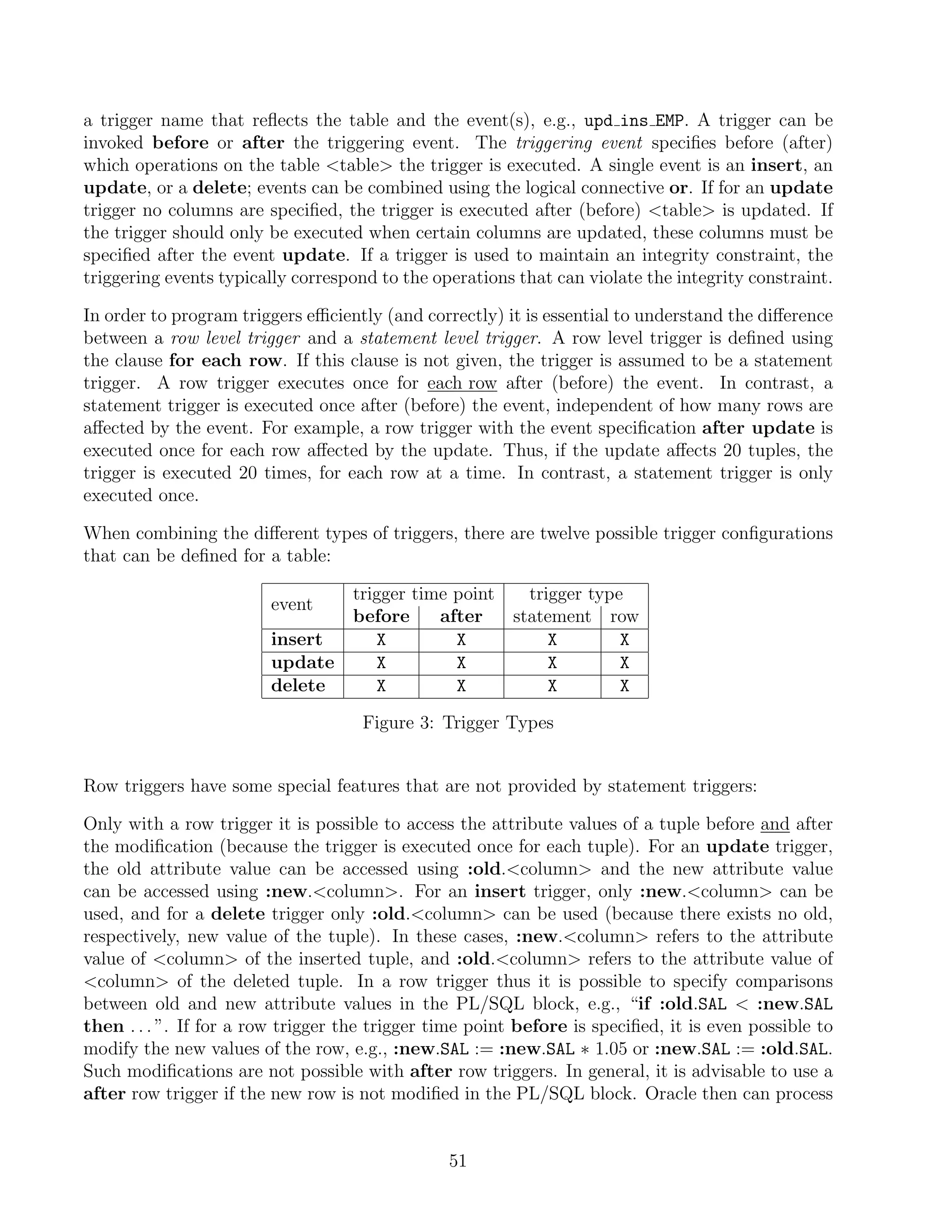
![these triggers more efficiently. Statement level triggers are in general only used in combination
with the trigger time point after.
In a trigger definition the when clause can only be used in combination with a for each row
trigger. The clause is used to further restrict when the trigger is executed. For the specification
of the condition in the when clause, the same restrictions as for the check clause hold. The
only exceptions are that the functions sysdate and user can be used, and that it is possible to
refer to the old/new attribute values of the actual row. In the latter case, the colon “:” must
not be used, i.e., only old.attribute and new.attribute.
The trigger body consists of a PL/SQL block. All SQL and PL/SQL commands except the
two statements commit and rollback can be used in a trigger’s PL/SQL block. Furthermore,
additional if constructs allow to execute certain parts of the PL/SQL block depending on the
triggering event. For this, the three constructs if inserting, if updating[(’column’)], and
if deleting exist. They can be used as shown in the following example:
create or replace trigger emp check
after insert or delete or update on EMP
for each row
begin
if inserting then
PL/SQL block
end if ;
if updating then
PL/SQL block
end if ;
if deleting then
PL/SQL block
end if ;
end;
It is important to understand that the execution of a trigger’s PL/SQL block builds a part of
the transaction that contains the triggering event. Thus, for example, an insert statement in
a PL/SQL block can cause another trigger to be executed. Multiple triggers and modifications
thus can lead to a cascading execution of triggers. Such a sequence of triggers terminates
successfully if (1) no exception is raised within a PL/SQL block, and (2) no declaratively
specified integrity constraint is violated. If a trigger raises an exception in a PL/SQL block,
all modifications up to the beginning of the transaction are rolled back. In the PL/SQL block
of a trigger, an exception can be raised using the statement raise application error (see
Section 4.1.5). This statement causes an implicit rollback. In combination with a row trigger,
raise application error can refer to old/new values of modified rows:
raise application error(−20020, ’Salary increase from ’ || to char(:old.SAL) || ’ to ’
to char(:new.SAL) || ’ is too high’); or
raise application error(−20030, ’Employee Id ’ ||
to char(:new .EMPNO) || ’ does not exist.’);
52](https://image.slidesharecdn.com/cfakepathkunalboss-226-1b02c961-9cd4-4a44-ae8a-48f5f1c614ab-091113025135-phpapp01/75/SQL-54-2048.jpg)