read

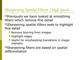
1. Sharpening Spatial Filters ( high pass)
Previously we have looked at smoothing
filters which remove fine detail
Sharpening spatial filters seek to highlight
fine detail
 Remove blurring from images
 Highlight edges
 Useful for emphasizing transitions in image
intensity
Sharpening filters are based on spatial
differentiation

2. Spatial Differentiation
Differentiation measures the rate of change
of a function
Let’s consider a simple 1 dimensional
example

3. Spatial Differentiation
A B

4. Spatial filters : Sharpening ( high pass)
1.LAPLACE
2.SOBEL

5. Spatial filters : Sharpening
1) LAPLACE
Laplace kernels

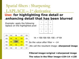
6. Use: for highlighting fine detail or
enhancing detail that has been blurred
.
153
157
156
153
155
159
156
158
156
159
155
158
154
156
160
154
157
158
160
160
157
157
157
156
155
Example: apply the following
laplace on the highlighted pixel
154
*
4
–
158
-
156-158-158
- =
14
So the value after filter = -14
We call the resultant image: sharpened image
.
Filtered image=original +sharpened image
The value in the filter image=154-14 =130
Spatial filters : Sharpening
LAPLACE – 1st
derivative

7. Spatial Fltering
LAPLACIAN

8. In the sharpened image , we may get negative value,
We deal with this case in 3 ways:
1.Covert negative value to zero (matlab does this)
2.Apply 2nd
derivative of laplace
1.Apply laplace again to the resultant sharpened
image
Spatial filters : Sharpening
LAPLACE – 1st
derivative

9. 153
157
156
153
155
159
156
158
156
159
155
158
154
156
160
154
157
158
160
160
157
157
157
156
155
Example: apply the following
laplace 2nd
derivative on the
highlighted pixel
Solution: apply laplace to all pixels
So the value after 2nd
derivative filter =-74
the value of pixel in the filter image=154-74 = 80
Spatial filters : Sharpening
LAPLACE – 2nd
derivative
154
*
4
–
158
-
156-158-158
- =
14
Then apply it again to our pixel:-14*4 – 10 -10 – (-6) -4 =-74

10. Spatial filters : Sharpening
1st
VS 2nd
derivative sharpening
1st
derivative sharpening produces thicker edges in an image
1st derivative sharpening has stronger response to gray level
change
2nd
derivative sharpening has stronger response to fine
details, such as thin lines and isolated points
.
2nd
derivative sharpening has double response to gray level
change

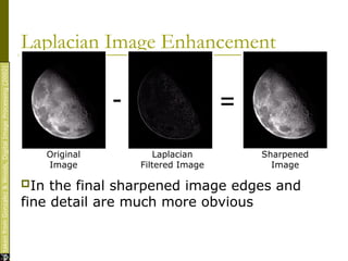
11. Laplacian Image Enhancement
In the final sharpened image edges and
fine detail are much more obvious
es
taken
from
Gonzalez
&
Woods,
Digital
Image
Processing
(2002)
- =
Original
Image
Laplacian
Filtered Image
Sharpened
Image

12. Laplacian Image Enhancement
es
taken
from
Gonzalez
&
Woods,
Digital
Image
Processing
(2002)

13. La place Sharpened image La place filtered image

14. Imfilter : for applying filter
.
Fspecial : for choosing the filter
:
Example: In MATLAB :
>> v=imread('picture2.jpg');
>> h=fspecial('laplacian‘,0);
>> Xp=imfilter(v,h);
>> imshow(Xp)
>> imshow(Xp+v)
Note: Xp=imfilter(x,p, ‘replicate‘)
This command will apply border padding instead of
zero padding
Laplacian Image Enhancement

15. Spatial filters : Sharpening
2) Sobel
Detects horizontal edges Detects vertical edges

16. Spatial filters : Sharpening
2) Sobel
we can apply the sobel horizontal kernel or the
sobel vertical kernel or both and adding them
together
.

17. Spatial filters : Sharpening
2) Sobel

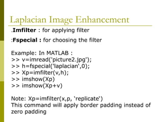
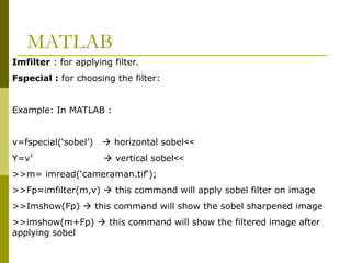
18. MATLAB
Imfilter : for applying filter.
Fspecial : for choosing the filter:
Example: In MATLAB :
>>
v=fspecial(‘sobel’)  horizontal sobel
>>
Y=v’  vertical sobel
>>m= imread(‘cameraman.tif‘);
>>Fp=imfilter(m,v)  this command will apply sobel filter on image
>>Imshow(Fp)  this command will show the sobel sharpened image
>>imshow(m+Fp)  this command will show the filtered image after
applying sobel

19. >>
imshow(v),figure,imshow(f+v)
;
>>
v=imread('picture2.jpg')
;
>>
h=fspecial('sobel')
;
>>
h1=h
;'
>>
p1=imfilter(v,h)
;
>>
p2=imfilter(v,h1)
;
>>
p3=abs(p1)+abs(p2)
;
>>
imshow(v),figure,imshow(p3+v)
;
Spatial filters : Sharpening
2) Sobel

20. Sharpening Filters:
Laplacian Sobel

21. Combining Spatial Enhancement Methods
Successful image
enhancement is typically
not achieved using a single
operation
Rather we combine a
range of techniques in order
to achieve a final result
This example will focus on
enhancing the bone scan to
the right

22. Combining Spatial Enhancement Methods
(cont…)
Images
taken
from
Gonzalez
&
Woods,
Digital
Image
Processing
(2002)
Laplacian filter of
bone scan (a)
Sharpened version
of bone scan
achieved by
subtracting (a)
and (b)
Sobel filter of
bone scan (a)
(a)
(b)
(c)
(d)

23. Combining Spatial Enhancement Methods
(cont…)
es
taken
from
Gonzalez
&
Woods,
Digital
Image
Processing
(2002)
The product of (c)
and (e) which will
be used as a mask
Sharpened image
which is sum of
(a) and (f)
Result of applying
apower-law
trans. to (g)
(
e
)
(
f
)
(
g
)
(
h
)
Image (d) smoothed
with a 5*5 averaging
filter

24. Combining Spatial Enhancement Methods
(cont…)
Compare the original and final images

25. Edge Tracing
b=rgb2gray(a); % convert to gray.
WE can only do edge tracing for gray
images
.
edge(b,'prewitt')
;
edge(b,'sobel')
;
edge(b,'sobel','vertical')
;
edge(b,'sobel','horizontal')
;
edge(b,'sobel','both')
;

26. Edge tracing
We can only do edge tracing using
gray scale images (i.e images without
color).
>> BW=rgb2gray(A);
>> edge(BW,’prewitt’)
That is what I saw
!
>>
edge(BW,’sobel’,’vertical’)
>>
edge(BW,’sobel’,’horizontal’)
>>
edge(BW,’sobel’,’both’)