This document provides the table of contents for the book "Soil Strength and Slope Stability" by J. Michael Duncan, Stephen G. Wright, and Thomas L. Brandon. The book contains 16 chapters that cover topics such as examples of slope failures, soil mechanics principles, stability conditions for analysis, shear strength of soils, methods for limit equilibrium analysis, reinforced slopes, rapid drawdown analysis, seismic slope stability, and slope stabilization techniques.


![DRAINED AND UNDRAINED SHEAR STRENGTHS 21
and the total stress after the load is applied would be
𝜎 = 𝜎0 + Δ𝜎 = 1.2 kPa + 19.4 kPa = 20.6 kPa (3.7)
The values of total stress are defined without reference to
how much of the force might be carried by contacts between
particles and how much is transmitted through water pres-
sure. Total stress is the same for the undrained and the drained
condition. The value of total stress depends only on equilib-
rium; it is equal to the total of all normal forces divided by
the total area.
When the load P is applied rapidly and the specimen is
undrained, the pore pressure changes. The specimen is con-
fined within the shear box and cannot deform. The clay is
saturated (the voids are filled with water), so the volume of
the specimen cannot change until water flows out. In this con-
dition, the added load is carried entirely by increased water
pressure. The soil skeleton (the framework or assemblage
of particles in contact with one another) does not change
shape, does not change volume, and carries none of the new
applied load.
Under these conditions the increase in water pressure is
equal to the change in total stress:
Δu = Δ𝜎 = 19.4 kPa (3.8)
where Δu is the increase in water pressure due to the change
in load in the undrained condition. The water pressure after
the load is applied is equal to the initial water pressure, plus
this change in pressure:
u = u0 + Δu = 0.5 kPa + 19.4 kPa = 19.9 kPa (3.9)
The effective stress is equal to the total stress [Eq. (3.7)]
minus the water pressure [Eq. (3.9)]:
𝜎′
= 20.6 kPa − 19.9 kPa = 0.7 kPa (3.10)
Because the increase in water pressure caused by the 200-N
load is equal to the increase in total stress, the effective stress
does not change.
The effective stress after the load is applied [Eq. (3.10)]
is the same as the effective stress before the load is applied
[Eq. (3.5)]. This is because the specimen is undrained. Water
does not have time to drain as the load is quickly applied, so
there is no volume change in the saturated specimen. As a
result the soil skeleton does not strain. The load carried by
the soil skeleton, which is measured by the value of effective
stress, does not change.
If the load is maintained over a period of time, drainage
will occur, and eventually the specimen will be drained. The
drained condition is achieved when there is no difference be-
tween the water pressures inside the specimen (the pore pres-
sure) and the water pressure outside, governed by the water
level in the reservoir around the direct shear apparatus. This
condition will be achieved (for practical purposes) in about
2 hours and will persist until the load is changed again.
After 2 hours, the specimen will have achieved 99 percent
equilibrium, the volume change will be essentially complete,
and the pore pressure on the horizontal plane will be equal to
the hydrostatic head at that level, u = 0.5 kPa.
In this drained condition, the effective stress is
𝜎′
= 20.6 kPa − 0.5 kPa = 20.1 kPa (3.11)
and all of the 200-N load is carried by the soil skeleton.
Recapitulation
• Total stress is the sum of all forces, including those
transmitted through particle contacts, and those
transmitted through water pressures, divided by
total area.
• Effective stress is equal to the total stress minus the
water pressure. It is the force transmitted through
particle contacts, divided by total area.
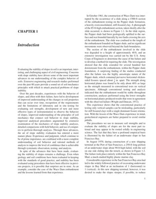
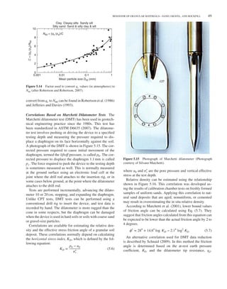
3.3 DRAINED AND UNDRAINED SHEAR
STRENGTHS
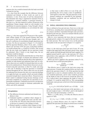
Shear strength is defined as the maximum value of shear
stress that the soil can withstand. The shear stress on the hor-
izontal plane in the direct shear test specimen in Figure 3.1
is equal to the shear force divided by the area:
𝜏 =
T
A
(3.12)
The shear strength of soils is controlled by effective stress,
no matter whether failure occurs under drained or undrained
conditions. The relationship between shear strength and
effective stress can be represented by a Mohr–Coulomb
strength envelope, as shown in Figure 3.2. The relation-
ship between s or 𝜏 and 𝜎′ shown in Figure 3.2 can be
expressed as
s = c′
+ 𝜎′
ff tan 𝜙′
(3.13)
where s is the shear strength, c′ is the effective stress cohe-
sion, 𝜎′
ff
is the effective stress on the failure plane at fail-
ure, and 𝜙′ is the effective stress angle of internal friction.
Effective stress envelopes may be curved to some degree.
This curvature, most important at low pressures, is discussed
in Chapters 5 and 6.
3.3.1 Sources of Shear Strength
If a shear load T is applied to the test specimen shown in
Figure 3.1, the top of the shear box will move to the left
relative to the bottom of the box. If the shear load is large
enough, the clay will fail by shearing on the horizontal plane,
and the displacement would be very large. Failure would
be accompanied by development of a rupture zone or break
through the soil, along the horizontal plane.](https://image.slidesharecdn.com/soilstrengthandslopestability-220624112511-a82802bd/85/Soil-Strength-and-Slope-Stability-pdf-37-320.jpg)


![BEHAVIOR OF GRANULAR MATERIALS—SAND, GRAVEL, AND ROCKFILL 39
0 percent corresponds to the minimum possible unit weight
(𝛾d-min). A relative density value of 100 percent corre-
sponds to the maximum possible unit weight (𝛾d-max). The
equation for relative density in terms of unit weight is shown
as Eq. (5.4):
Dr =
𝛾d−max
𝛾d
⋅
[
𝛾d − 𝛾d−min
𝛾d−max − 𝛾d−min
]
⋅ 100% (5.4)
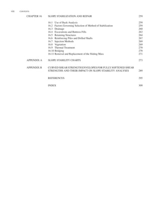
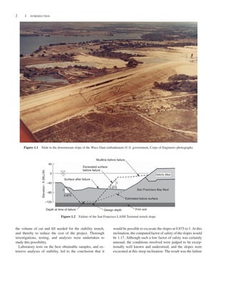
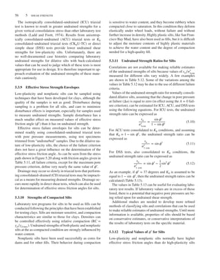
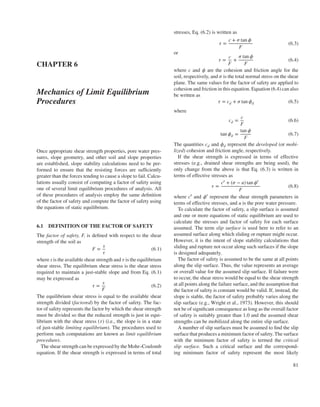
Values of 𝜙′ increase with density. The value of 𝜙0
increases by about 10 degrees as the density varies from
the loosest to the densest state. Values of Δ𝜙 also in-
crease as density increases, ranging from about 3 degrees
for loose materials to about 7 degrees for dense materials.
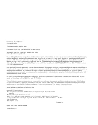
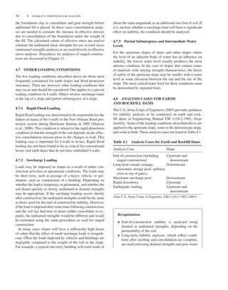
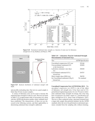
An example is shown in Figure 5.3, for Sacramento River
sand, a uniformly graded fine sand composed predominantly
of feldspar and quartz particles. At a confining pressure of
1 atm, 𝜙0 increases from 35 degrees for Dr = 38 percent
to 44 degrees for Dr = 100 percent. The value of Δ𝜙 in-
creases from 2.5 degrees for Dr = 38 percent to 7 degrees for
Dr = 100 percent.
5.2.3 Effects of Gradation
All other things being equal, values of 𝜙′ are higher for
well-graded granular soils like the Oroville Dam shell mate-
rial (Figures 5.1 and 5.2) than for uniformly graded soils like
Sacramento River sand (Figure 5.3). In well-graded soils,
smaller particles fill gaps between larger particles, and as a
result it is possible to form a more dense packing that offers
greater resistance to shear. Well-graded materials are subject
to segregation of particle sizes during fill placement and may
form fills that are stratified, with alternating coarser and finer
layers unless care is taken to ensure that segregation does not
occur during fill placement.
30
0.1 1 10 0
0 100
Effective normal stress on failure plane (kPa)
200 300 400
100
Shear
stress
on
failure
plane
at
failure,
τ
(kPa)
Max. particle size = No. 50 sieve
Specimen diam. = 35.6 mm
200
300
Dr = 100%
ϕ0 = 44 degrees
∆ϕ = 7 degrees
Dr = 38%
ϕ0 = 35.2 degrees
∆ϕ = 2.5 degrees
Sacramento River Sand
Sacramento River Sand
D r
=
100%
Dr
= 38%
35
40
Angle
of
internal
friction,
ϕ′
45
Effective confining pressure
Atmospheric pressure pa
log scale
– –
σ3′
(a) (b)
Figure 5.3 Effect of density on strength of Sacremento River sand: (a) variations of 𝜙′
with 𝜎′
3
and (b) strength envelopes.
Data from Lee and Seed (1967).
5.2.4 Plane Strain Effects
Most laboratory strength tests are performed using triax-
ial equipment, where a circular cylindrical test specimen is
loaded axially and deforms with radial symmetry. In con-
trast, the deformations for many field conditions are close to
plane strain. In plane strain, all displacements are parallel to
one plane. In the field, this is usually a vertical plane. Strains
and displacements perpendicular to this plane are zero. For
example, in a long embankment, symmetry requires that all
displacements be in vertical planes perpendicular to the lon-
gitudinal axis of the embankment.
The value of 𝜙′ for plane strain conditions (𝜙′
ps) is higher
than the value for triaxial conditions (𝜙′
t). Becker et al. (1972)
found that the value of 𝜙′
ps was 1 to 6 degrees larger than the
value of 𝜙′
t for the same material at the same density, tested
at the same confining pressure. The difference was greatest
for dense materials tested at low pressures. For confining
pressures less than 100 psi, they found that 𝜙′
ps was 3 to 6
degrees larger than 𝜙′
t.
Although there may be a significant difference between
values of 𝜙′ measured in triaxial tests and the values most
appropriate for field conditions close to plane strain, this dif-
ference is usually ignored. It is conservative to ignore the
difference and use triaxial values of 𝜙′ for plane strain con-
ditions. This conventional practice provides an intrinsic addi-
tional safety margin for situations where the strain boundary
conditions are close to plane strain.
5.2.5 Triaxial Tests on Granular Materials
Minimum Specimen Size For design of major struc-
tures such as dams, triaxial tests performed on specimens
compacted to the anticipated field density are frequently](https://image.slidesharecdn.com/soilstrengthandslopestability-220624112511-a82802bd/85/Soil-Strength-and-Slope-Stability-pdf-55-320.jpg)


![BEHAVIOR OF GRANULAR MATERIALS—SAND, GRAVEL, AND ROCKFILL 43
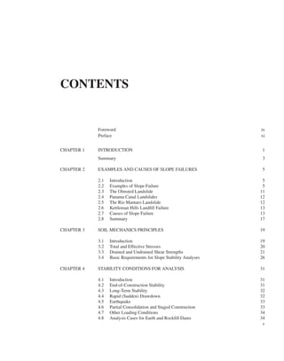
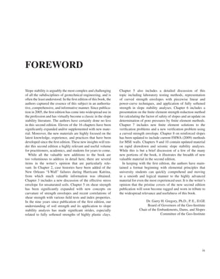
Table 5.4 Correlation between Fiction Angle, Gradation Characteristics, Relative Density, and Confining Pressure
for Sands, Gravels, and Rockfills
𝝓′
= A + B(Dr) −
[
C + D
(
Dr
)]
log10
(
𝝈′
N
pa
)
Parameter Values in Degrees
A B C D
Standard Deviation
(deg)
Gravel and cobbles with Cu > 4 44 10 7 2 3.1
Sand with Cu > 6 39 10 3 2 3.2
Sand with Cu < 6 34 10 3 2 3.2
• Friction angles increase as density increases. This is re-
flected in the value of the parameter B, which indicates
that 𝜙′ increases by 10 degrees as Dr varies from 0 to
100 percent.
• Friction angles decrease logarithmically with increas-
ing normal pressure. This is reflected by the values of
C, which indicates a larger effect for gravel and cobbles
than for sand, and D, which has the same small effect
for all the materials.
By accounting for the effects of density and gradation,
the standard deviation of the correlation is reduced from 4.5
degrees for the trend line shown in Figure 5.6 to slightly over
3 degrees for the correlation equation shown in Table 5.4. The
remaining scatter in the data is due to variables that are not
reflected in the correlation, such as particle strength, particle
shape, and surface roughness. Although these factors are not
readily quantifiable, they cause appreciable variations in the
measured values of 𝜙′.
The value of the normal stress, 𝜎′
N
, in the equation shown
in Figure 5.6 is related to 𝜎′
3
by the following equation:
𝜎′
N
𝜎′
3
=
cos2𝜙
1 − sin 𝜙
= 2sin2
(
45 +
𝜙′
2
)
(5.5)
Values of 𝜎′
N
∕𝜎′
3
vary with 𝜙′ as follows:
𝜙′
(deg)
𝜎′
N
𝜎′
3
30 1.50
40 1.64
50 1.77
60 1.87
This relationship facilitates relating laboratory conditions,
where 𝜎′
3
is known, to field conditions and slope stability
analyses, where 𝜎′
N
is known.
In slope stability analyses, the value of 𝜎′
N
can be deter-
mined from examination of the values of normal stress on the
bases of slices. The effective normal stress should be used
for this purpose. The value of 𝜎′
N
varies from slice to slice
around a slip surface. This variation can be accommodated
in a number of ways:
1. Use an estimated average value of 𝜎′
N
in the correlation
equation.
2. Use the maximum value of 𝜎′
N
in the correlation
equation. This results in the lowest value of 𝜙 around
the slip surface and is therefore conservative.
3. Use a slope stability computer program that is able to
represent variation of shear strength with normal stress.
This involves the least approximation.
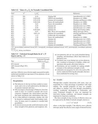
Comparisons of Correlations with Test Data The follow-
ing comparisons of measured and estimated values of 𝜙′
illustrate the use of the correlation equation for gravel and
uniformly graded sand:
1. VDOT 21B gravel [tests by Duncan et al. (2007)].
With 43 percent passing the No. 4 sieve, Cu = 64 to
95, Dr = 75 percent, 𝜎′
N
= 20 psi.
𝜙estimated = 44 + (10)(0.75)
−
[
7 + (2) (0.75) log
35
14.7
]
degrees
𝜙estimated = 44degrees
𝜙measured = 45degrees
2. Uniformly graded silica sand [tests by Duncan and
Chang (1970)].
With 100 percent passing the No. 4 sieve, Cu < 6,
Dr = 75 percent, 𝜎′
N
= 4.5 atm.
𝜙estimated = 34 + (10)(0.90)
−
[
3 + (2) (0.90) log
4.5
1.0
]
degrees
𝜙estimated = 39degrees
𝜙measured = 37degrees](https://image.slidesharecdn.com/soilstrengthandslopestability-220624112511-a82802bd/85/Soil-Strength-and-Slope-Stability-pdf-59-320.jpg)
![44 5 SHEAR STRENGTH
Table 5.5 Probabilities of Overestimating Friction
Angle as a Function of Standard Deviations
Probability Actual Value of 𝜙 Could Be
Smaller Than the Value Estimated
Using Table 5.4
Number of
Standard
Deviations
below Value
Estimated
Using
Table 5.4.
Normal
Distribution
(%)
Lognormal
Distribution
(%)
0 50 50
1 16 16
2 2 2
3 0.1 0.1
Significance of Standard Deviation. The differences
between measured values of 𝜙′ and values computed using
the equation in Table 5.4 are approximated reasonably well
by either normal or lognormal distributions. Either of these
distributions can be used to estimate the reliability of values
of 𝜙′ estimated using the equation. The possibility that the
value of 𝜙 could be overestimated by the correlation equation
can be judged based on the relationships shown in Table 5.5.
Thus, for the VDOT 21B gravel considered in the example
above, the likelihood that the friction angle might be less
than 41 degrees (44 degrees minus one standard deviation)
is 16 percent. For the well-graded silica sand considered in
the second example, the likelihood that the friction angle
might be less than 36 degrees (39 degrees minus one standard
deviation) is also 16 percent.
The often-used “two-thirds rule” for evaluating strength
test results (choosing the design value such that two-thirds
of the measured values are higher and one-third are lower)
corresponds to a value about one-half of a standard deviation
below the average, which, for these estimates of friction
angles for granular materials, is about 1.5 degrees below
the average estimated value. Probability theory indicates that
there is a 31 percent chance that the actual strength will be
lower than a design value selected using the two-thirds rule.
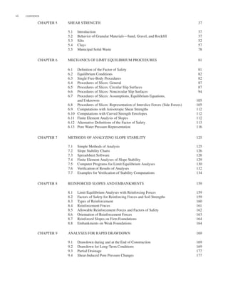
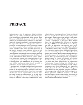
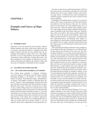
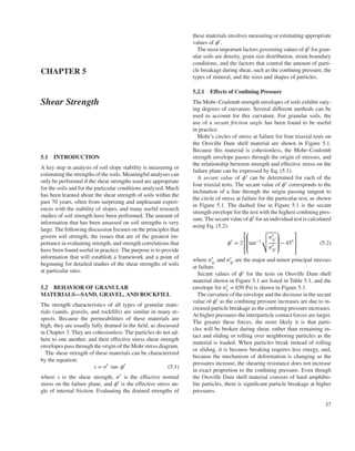
Correlations Based on Standard Penetration Tests The
standard penetration test is a commonly used in situ test in
geotechnical engineering practice. The test is performed by
Split Tube
Ball Check
Shoe
Hardened
Figure 5.7 Cross section of split-spoon sampler (Acker, 1974).Cross section of splitCross section of
split
driving a standard split-spoon or split-barrel sampler [2-in.
OD (outer diameter) and 1.375-in. ID (inner diameter)] into
the soil at the bottom of a borehole a distance of 18 in.,
using a drop hammer weighing 140 lb, falling 30 in. A cross
section of a split-spoon sampler is shown in Figure 5.7. The
number of blows required to drive the sampler the final 12 in.
(from 6 in. penetration to 18 in. penetration) is the SPT blow
count, N.
For use in estimating soil properties based on SPTs, blow
counts are usually standardized in two ways:
1. Various hammer systems involve different amounts of
energy loss and, therefore, deliver different amounts of
energy to the sampler. Blow counts are usually adjusted
to a standard 60 percent of the theoretical energy of the
140-lb hammer falling 30 in. This adjusted blow count
is called N60.
2. Blow counts increase with overburden pressure, even
though the relative density may be the same. For this
reason blow counts are sometimes adjusted to a stan-
dard overburden pressure of 1.0 atm or 1.0 ton per
square foot (tsf). This adjusted blow count is called
N1,60.
Further details regarding SPTs can be found in McGregor
and Duncan (1998) and ASTM D1586 (2011).
Friction angles for granular soils can be estimated using
the SPT in two different ways. First, the relative density
of the granular deposit can be estimated based on the SPT
blow count. The resulting relative density can then be used in
correlations of the type described in the previous section. As
an example, Figure 5.8 can be used to estimate in situ relative
density based on SPT blow count. This relative density can
be used in conjunction with grain size information measured
using the disturbed sample obtained with the split-spoon
sampler during the SPT, to estimate 𝜙0 and Δ𝜙 using the
correlation shown in Table 5.4.
Many other correlations are available to estimate relative
density based on SPT blow count. A summary of these cor-
relations is given in Table 5.6. These correlations take into
account the vertical effective stress at the depth of the blow
count measurement. This is important because relative den-
sity varies with both blow count and vertical pressure, as
shown in Figure 5.8.](https://image.slidesharecdn.com/soilstrengthandslopestability-220624112511-a82802bd/85/Soil-Strength-and-Slope-Stability-pdf-60-320.jpg)


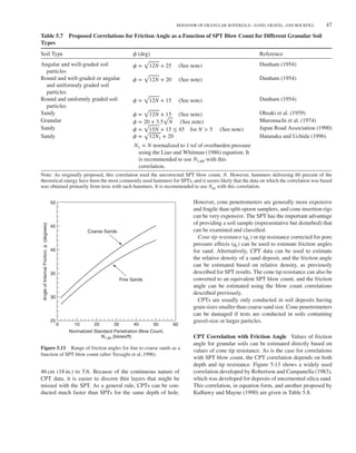
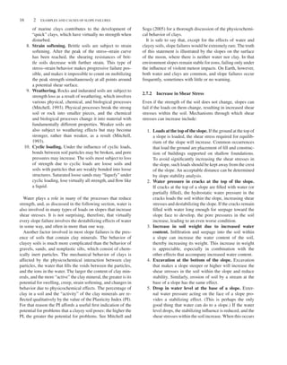
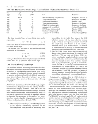
![48 5 SHEAR STRENGTH
Figure 5.12 Cone penetrometers: 15 cm2
cone on the left and
10 cm2
cone on the right.
0
30° 32° 34° 36° 38° 40°
42°
44°
46°
ϕ′ = 48°
4.0
3.5
3.0
2.5
Vertical
Effective
Stress,
σ′
v
(kgf/cm
2
)
2.0
1.5
1.0
0.5
0.0
100 200 300
Cone Tip Resistance, qc (kgf/cm2
)
400 500
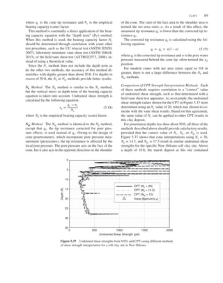
Figure 5.13 Correlation of friction angle with CPT tip resistance
as a function of vertical effective stress (after Robertson and Cam-
panella, 1983). Copyright 2008 Canadian Science Publishing. Re-
produced with permission.
CPT Correlations to Relative Density Many of the corre-
lations developed for CPTs are based on results from labora-
tory tests conducted in calibration chambers with uniformly
Table 5.8 Correlations of Friction Angle with CPT Tip
Resistance for Granular Soils
Equation Reference
𝜙′ = arctan
[
1
2.68
[
log
(
qc
𝜎′
v
)]
+ 0.29
]
Robertson and
Campanella
(1983)
𝜙′ = 17.6 + 11 log
(
qc
√
𝜎′
v
)
Kulhawy and
Mayne (1990)
log = logarithm to base 10.
Note: qc and 𝜎′
v values are in tons per square foot (tsf), atmospheres,
or kg/cm2
.
Table 5.9 Correlations of Relative Density to CPT Tip
Resistance
Equation Reference
Dr = 100
⎡
⎢
⎢
⎢
⎣
(
qc∕
√
𝜎′
v
)
305
⎤
⎥
⎥
⎥
⎦
1∕2 Kulhawy and
Mayne (1990)
Dr = −1.292 + 0.268 ln
(
qc∕
√
𝜎′
v
)
Jamiolkowski
et al. (1985)
Dr =
1
2.41
ln
(
qc∕
√
𝜎′
v
15.7
)
Baldi et al. (1986)
Dr =
100
2.91
ln
(
qc
61𝜎′ 0.71
v
)
Lunne and
Christofferson
(1983)
Dr = 100
[
0.268 ln
(
qc∕
√
𝜎′
v
)
− 0.675
]
Jamiolkowski
et al. (2001)
ln = natural logarithm.
Note: qc and 𝜎′
v values are in tons per square foot (tsf), atmospheres,
or kg/cm2
.
graded sands. Examples of correlations that are used in prac-
tice to estimate relative density are given in Table 5.9. Since
natural deposits of sand are often nonuniform, may contain
fines, and have undergone varying degrees of aging, these
correlations should be considered approximate.
CPT Correlations with SPT Blow Count Many engineers
have been more comfortable with converting CPT results to
equivalent SPT blow count and then using the blow count in
correlations for which they have experience and confidence.
The data in Figure 5.14 can be used to convert CPT tip
resistance to an equivalent value of N60. The measured value
of qc (in atmospheres, or tons/ft2, or kg/cm2) is divided by
the value of C to find the equivalent N60. Other methods to](https://image.slidesharecdn.com/soilstrengthandslopestability-220624112511-a82802bd/85/Soil-Strength-and-Slope-Stability-pdf-64-320.jpg)


![MUNICIPAL SOLID WASTE 79
Open points - 300 to 1500 mm
direct shear tests
Solid points - back analysis of
failed slopes
350
250
150
50
0
0 50 100 200
Normal Stress (kPa)
Shear
Strength
(kPa)
300
35°
Average
400
150 250 350
300
200
100
Figure 5.50 Range of shear strength envelopes for municipal solid
waste based on large-scale direct shear tests and back analysis of
failed slopes (after Eid et al., 2000).
slopes in waste to develop the range of strength envelopes
show in Figure 5.50. All three envelopes (lower bound, av-
erage, and upper bound) are inclined at 𝜙 = 35 degrees.
The average envelope shown in Figure 5.48 corresponds
to c = 25 kPa, and the lowest of the envelopes corresponds
to c = 0.
Based on review of published information on MSW, Bray
et al. (2008, 2009) concluded that fibrous materials tend to
become oriented with their long dimensions horizontal or
subhorizontal. The strength of the waste is smaller when the
failure plane is horizontal (parallel to the fibrous materials),
than when the failure plane cuts across the fibrous materials.
As a result, strengths measured in direct shear tests, where
the failure plane is horizontal, are smaller than strengths
measured in triaxial tests, where failure planes are oriented
at about 60 degrees to horizontal.
Bray et al. (2008, 2009) also found that failure envelopes
for MSW are curved to some degree, and that friction angles
decreased with increasing pressure. They concluded that a
reasonable mean estimate of the shear strength of MSW for
use in preliminary stability evaluations can be expressed as
s = c + 𝜎n tan
[
𝜙0 − Δ𝜙 log10
(
𝜎n
pa
)]
(5.26)
where
s = shear strength in the same units as 𝜎n
c = cohesion intercept = 15 kPa
𝜎n = normal stress on failure plane
𝜙0 = 36 degrees = friction angle for 𝜎n = 1.0 atm
Δ𝜙 = 5 degrees = reduction in friction angle for 10-fold
increase in 𝜎n
pa = atmospheric pressure = 101 kPa
Equation (5.26) applies to shear planes parallel to the fi-
brous material orientation, where the shear strength is lowest.](https://image.slidesharecdn.com/soilstrengthandslopestability-220624112511-a82802bd/85/Soil-Strength-and-Slope-Stability-pdf-95-320.jpg)


![Duncan c06.tex V3 - 07/21/2014 4:38 P.M. Page˜83
SINGLE FREE-BODY PROCEDURES 83
A W
S
N
Aʹ
Bʹ
z
B
β
ℓ
Figure 6.1 Infinite slope and plane slip surface.
forces on the ends of the block exactly balance each other and
can be ignored in the equilibrium equations. Summing forces
in directions perpendicular and parallel to the slip plane gives
the following expressions for the shear force, S, and normal
force, N, on the plane:
S = W sin 𝛽 (6.9)
N = W cos 𝛽 (6.10)
where 𝛽 is the angle of inclination of the slope and slip
plane, measured from the horizontal, and W is the weight
of the block. For a block of unit thickness in the direction
perpendicular to the plane of the cross section in Figure 6.1,
the weight is expressed as
W = 𝛾𝓁z cos 𝛽 (6.11)
where 𝛾 is the total unit weight of the soil, 𝓁 is the distance
between the two ends of the block, measured parallel to
the slope, and z is the depth of the shear plane, measured
vertically. Substituting Eq. (6.11) into Eqs. (6.9) and (6.10)
gives
S = 𝛾𝓁z cos 𝛽 sin 𝛽 (6.12)
N = 𝛾𝓁z cos2
𝛽 (6.13)
The shear and normal stresses on the shear plane are constant
for an infinite slope and are obtained by dividing Eqs. (6.12)
and (6.13) by the area of the plane (𝓁 ⋅ 1) to give
𝜏 = 𝛾z cos 𝛽 sin 𝛽 (6.14)
𝜎 = 𝛾z cos2
𝛽 (6.15)
Substituting these expressions for the stresses into Eq. (6.3)
for the factor of safety for total stresses gives
F =
c + 𝛾z cos2𝛽 tan 𝜙
𝛾z cos 𝛽 sin 𝛽
(6.16)
For effective stresses, the equation for the factor of safety
becomes
F =
c′ + (𝛾z cos2𝛽 − u) tan 𝜙′
𝛾z cos 𝛽 sin 𝛽
(6.17)
z
β
γ
c, ϕ
or
cʹ, ϕʹ, u
Total Stresses: s = c + 𝜎 tan 𝜙
Subaerial (not submerged) slopes:
F =
c
𝛾 z
2
sin(2𝛽)
+ [cot 𝛽] tan 𝜙
Submerged slopes (𝜙 = 0 only):
F =
c
(𝛾 − 𝛾w)z
2
sin(2𝛽)
Effective Stresses: s = c′ + 𝜎′ tan 𝜙′
General case (subaerial slope):
F =
c′
𝛾z
2
sin(2𝛽)
+
[
cot 𝛽 −
u
𝛾z
(cot 𝛽 + tan 𝛽)
]
tan 𝜙′
Submerged slopes—no flow:
F =
c′
(𝛾 − 𝛾w)z
2
sin(2𝛽)
+ [cot 𝛽] tan 𝜙′
Subaerial slope—seepage parallel to slope face:
F =
c′
𝛾z
2
sin(2𝛽)
+
[
cot 𝛽 −
𝛾w
𝛾
(cot 𝛽)
]
tan 𝜙′
Subaerial slope—horizontal seepage:
F =
c′
𝛾z
2
sin(2𝛽)
+
[
cot 𝛽 −
𝛾w
𝛾
(cot 𝛽 + tan 𝛽)
]
tan 𝜙′
Subaerial slope—pore water pressures defined by a con-
stant value of ru = u
𝛾z
:
F =
c′
𝛾z
2
sin(2𝛽)
+ [cot 𝛽 − ru(cot 𝛽 + tan 𝛽)] tan 𝜙′
Figure 6.2 Equations for computing the factor of safety for an
infinite slope.
Equations for computing the factor of safety for an infinite
slope are summarized in Figure 6.2 for both total stress and
effective stress analyses and a variety of water and seepage
conditions.
For a cohesionless (c = 0, c′ = 0) soil, the factor of safety
calculated by an infinite slope analysis is independent of the
depth, z, of the slip surface. For total stresses (or effective
stresses with zero pore water pressure) the equation for the
factor of safety becomes
F =
tan 𝜙
tan 𝛽
(6.18)](https://image.slidesharecdn.com/soilstrengthandslopestability-220624112511-a82802bd/85/Soil-Strength-and-Slope-Stability-pdf-99-320.jpg)
![Duncan c06.tex V3 - 07/21/2014 4:38 P.M. Page˜84
84 6 MECHANICS OF LIMIT EQUILIBRIUM PROCEDURES
Similarly for effective stresses, if the pore water pressures
are proportional to the depth of the slip plane, the factor of
safety is expressed by
F = [cot 𝛽 − ru(cot 𝛽 + tan 𝛽)] tan 𝜙′
(6.19)
where ru is the pore water pressure coefficient suggested by
Bishop and Morgenstern (1960). The value of ru is defined
as
ru =
u
𝛾z
(6.20)
Because the factor of safety for a cohesionless slope is inde-
pendent of the depth of the slip surface, a slip surface that
is only infinitesimally deep has the same factor of safety
as that for deeper surfaces. Thus the infinite slope analy-
sis procedure is the appropriate procedure for any slope in
cohesionless soil.1
The infinite slope analysis is also applicable to slopes in
cohesive soils provided that a firmer stratum parallel to the
face of the slope limits the depth of the failure surface. If such
a stratum exists at a depth that is small compared to the
lateral extent of the slope, an infinite slope analysis provides
a suitable approximation for stability calculations.
The infinite slope equations were derived by consider-
ing equilibrium of forces in two mutually perpendicular
directions and thus satisfy all force equilibrium require-
ments. Moment equilibrium was not considered explicitly.
However, the forces on the two ends of the block are collinear
and the normal force acts at the center of the block. Thus,
moment equilibrium is satisfied, and the Infinite Slope pro-
cedure can be considered to satisfy all the requirements for
static equilibrium.
Recapitulation
• For a cohesionless slope, the factor of safety is in-
dependent of the depth of the slip surface, and thus
an infinite slope analysis is appropriate (exceptions
occur for curved Mohr failure envelopes).
• For cohesive soils, the infinite slope analysis proce-
dure may provide a suitable approximation provided
that the slip surface is parallel to the slope and lim-
ited to a depth that is small compared to the lateral
dimensions of the slope.
• The infinite slope analysis procedure fully satisfies
static equilibrium.
1An exception to this for soils with curved Mohr failure envelopes that pass
through the origin. Although there is no strength at zero normal stress, and
thus the soil might be termed cohesionless, the factor of safety depends on
the depth of slide and the infinite slope analysis may not be appropriate. Also
see the example of the Oroville Dam presented in Chapter 7.
6.3.2 Logarithmic Spiral Procedure
In the Logarithmic Spiral procedure, the slip surface is as-
sumed to be a Logarithmic Spiral, as shown in Figure 6.3
(Frohlich, 1953). A center point, an initial radius, r0, and a
value of 𝜙d define the spiral. The radius of the spiral varies
with the angle of rotation, 𝜃, about the center of the spiral
according to the expression
r = r0e𝜃 tan 𝜙d (6.21)
where 𝜙d is the developed friction angle. The value of 𝜙d
depends on the friction angle of the soil and the factor of
safety, as shown by Eq. (6.7). The stresses along the slip
surface consist of the normal stress (𝜎) and the shear stress
(𝜏). For total stress analyses, the shear stress can be expressed
in terms of the normal stress, the shear strength parameters
(c and 𝜙), and the factor of safety. From Eq. (6.4),
𝜏 =
c
F
+ 𝜎
tan 𝜙
F
(6.22)
or in terms of developed shear strengths,
𝜏 = cd + 𝜎 tan 𝜙d (6.23)
A log spiral has the properties that the radius extended
from the center of the spiral to a point on the slip surface
intersects the slip surface at an angle, 𝜙d, to the normal
(Figure 6.3). Because of this property, the resultant forces
produced by the normal stress (𝜎) and the frictional por-
tion of the shear stress (𝜎 tan 𝜙d) act along a line through
the center of the spiral and produce no net moment about
the center of the spiral. The only forces on the slip surface
that produce moments about the center of the spiral are those
due to the developed cohesion. An equilibrium equation
may be written by summing moments about the center of
the spiral, which involves the factor of safety as the only
Center point
r0
r = r0 eθ tan ϕ
d
θ
ϕd
τ
σ
Figure 6.3 Slope and Logarithmic Spiral slip surface (after
Frohlich, 1953).](https://image.slidesharecdn.com/soilstrengthandslopestability-220624112511-a82802bd/85/Soil-Strength-and-Slope-Stability-pdf-100-320.jpg)
![Duncan c06.tex V3 - 07/21/2014 4:38 P.M. Page˜85
SINGLE FREE-BODY PROCEDURES 85
unknown. This equation may be used to compute the factor
of safety.
In the Logarithmic Spiral procedure a statically determi-
nant solution is achieved by assuming a particular shape
(Logarithmic Spiral) for the slip surface. By assuming a
Logarithmic Spiral, no additional assumptions are required.
Force equilibrium is not considered explicitly in the Loga-
rithmic Spiral procedure. However, there are an infinite num-
ber of combinations of normal and shear stresses along the
slip surface that will satisfy force equilibrium. All of these
combinations of shear and normal stress will yield the same
value for the factor of safety. Thus, the Logarithmic Spiral
implicitly satisfies complete static equilibrium. The Loga-
rithmic Spiral and Infinite Slope procedures are the only two
limit equilibrium procedures that satisfy complete equilib-
rium by assuming a specific shape for the slip surface.
Because the Logarithmic Spiral procedure fully satisfies
static equilibrium, it is accurate in terms of mechanics.
Also, for homogeneous slopes, a Logarithmic Spiral appears
to approximate the shape of the most critical potential slid-
ing surface reasonably well. Thus from a theoretical point of
view, the logarithmic spiral procedure is the best limit equi-
librium procedure for analyses of homogeneous slopes.
For cohesionless (c, c′ = 0) slopes the critical Logarithmic
Spiral that produces the minimum factor of safety has an
infinite radius and the spiral coincides with the face of the
slope (Figure 6.4). In this case the Logarithmic Spiral and
Infinite Slope procedures produce identical values for the
minimum factor of safety.
The Logarithmic Spiral equations are relatively complex
and awkward for hand calculations because of the assumed
shape of the slip surface. However, the Logarithmic Spiral
procedure is computationally efficient and well suited for
implementation in computer calculations. The procedure is
useful for performing the computations required to produce
slope stability charts, and once such charts have been de-
veloped, there is little need for using the detailed Logarith-
mic Spiral equations (Wright, 1969; Leshchinsky and Volk,
1985; Leshchinsky and San, 1994). The Logarithmic Spi-
ral procedure has also received recent interest and attention
for use in software to analyze reinforced slopes, particularly
for design software that must perform many repetitive cal-
culations to find a suitable arrangement for reinforcement
(Leshchinsky, 1997).
Recapitulation
• The Logarithmic Spiral procedure achieves a stati-
cally determinate solution by assuming a Logarith-
mic Spiral shape for the slip surface [Eq. (6.21)].
• The Logarithmic Spiral procedure explicitly sat-
isfies moment equilibrium and implicitly satisfies
force equilibrium. Because equilibrium is fully
Critical slip surface
r ≈ ∞
ϕd = β
ϕd = β
β
Figure 6.4 Critical Logarithmic Spiral slip surface for a cohesion-
less slope.
satisfied, the procedure is accurate with regard to
mechanics.
• The Logarithmic Spiral procedure is theoretically
the best procedure for analysis for homogeneous
slopes. The effort involved in applying it can be re-
duced by use of dimensionless slope stability charts
(Leshchinsky and Volk, 1985; Leshchinsky and San,
1994).
• The Logarithmic Spiral procedure is used in several
computer programs for design of reinforced slopes
using geogrids, soil nails, and so on.
6.3.3 Swedish Circle (𝝓 = 𝟎) Method
In the Swedish Circle method the slip surface is assumed to
be a circular arc and moments are summed about the center
of the circle to calculate a factor of safety. Some form of
the method was apparently first used by Petterson in about
1916 (Petterson, 1955), but the method seems to have first
been formalized for 𝜙 = 0 by Fellenius in 1922 (Fellenius,
1922; Skempton, 1948). The friction angle is assumed to be
zero, and thus the shear strength is assumed to be due to
“cohesion” only. For this reason, the Swedish Circle method
is also called the 𝜙 = 0 method.
The Swedish Circle or 𝜙 = 0 method is actually a special
case of the Logarithmic Spiral procedure: When 𝜙 = 0, a](https://image.slidesharecdn.com/soilstrengthandslopestability-220624112511-a82802bd/85/Soil-Strength-and-Slope-Stability-pdf-101-320.jpg)


![Duncan c06.tex V3 - 07/21/2014 4:38 P.M. Page˜88
88 6 MECHANICS OF LIMIT EQUILIBRIUM PROCEDURES
where Si is the shear force on the base of the ith slice
and the summation is performed for all slices. The shear
force is the product of the shear stress, 𝜏i, and the area of
the base of the slice, which for a slice of unit thickness is
Δ𝓁i ⋅ 1. Thus,
Mr = r
∑
𝜏i Δ𝓁i (6.36)
The shear stress can be expressed in terms of the shear
strength and the factor of safety by Eq. (6.1) to give
Mr = r
∑ si Δ𝓁i
F
(6.37)
where si is the strength of the soil at the base of slice i.
Equating the resisting moment [Eq. (6.37)] and the driving
moment [Eq. (6.34)] and rearranging, the following equation
can be written for the factor of safety:
F =
∑
si Δ𝓁i
∑
Wi sin 𝛼i
(6.38)
The radius has been canceled from both the numerator and
denominator of this equation. However, the equation is still
valid only for a circular slip surface.
At this point the subscript i will be dropped from use with
the understanding that the quantities inside the summation
are the values for an individual slice and that the summations
are performed for all slices. Thus, Eq. (6.38) is written as
F =
∑
s Δ𝓁
∑
W sin 𝛼
(6.39)
For total stresses the shear strength is expressed by
s = c + 𝜎 tan 𝜙 (6.40)
Substituting this into Eq. (6.39), gives
F =
∑
(c + 𝜎 tan 𝜙)Δ𝓁
∑
W sin 𝛼
(6.41)
Equation (6.41) represents the static equilibrium equation
for moments about the center of a circle. If 𝜙 is equal to zero,
Eq. (6.41) becomes
F =
∑
c Δ𝓁
∑
W sin 𝛼
(6.42)
which can be solved for a factor of safety. Equations (6.42)
and (6.31), derived earlier for the Swedish Circle (𝜙 = 0)
method, both satisfy moment equilibrium about the center
of a circle and make no assumptions other than that 𝜙 = 0
and that the slip surface is a circle. Therefore, both equations
produce the same value for the factor of safety. The only
difference is that Eq. (6.31) considers the entire free body as
a single mass, and Eq. (6.42) considers the mass subdivided
into slices. Equation (6.42) is more convenient to use than
Eq. (6.31) because it avoids the need to locate the center of
gravity of what may be an odd-shaped soil mass above the
slip surface.
If the friction angle is not equal to zero, Eq. (6.41) re-
quires that the normal stress on the base of each slice be
known. The problem of determining the normal stress is stat-
ically indeterminate and requires that additional assumptions
be made in order to compute the factor of safety. The Ordi-
nary Method of Slices and the Simplified Bishop procedures
described in the next two sections make two different sets of
assumptions to obtain the normal stress on the base of the
slices and, subsequently, the factor of safety.
6.5.1 Ordinary Method of Slices
The Ordinary Method of Slices is a procedure of slices that
neglects the forces on the sides of the slices. The Ordinary
Method of Slices has also been referred to as the “Swedish
Method of Slices” and the “Fellenius method.” This method
should not, however, be confused with the U.S. Army Corps
of Engineers’ Modified Swedish method, which is described
later. Similarly, the method should not be confused with
other methods of slices that Fellenius developed, includ-
ing a method of slices that fully satisfies static equilibrium
(Fellenius, 1936).
Referring to the slice shown in Figure 6.8 and resolving
forces perpendicular to the base of the slice, the normal force
for the Ordinary Method of Slices can be expressed as
N = W cos 𝛼 (6.43)
The normal force expressed by Eq. (6.43) is the same as the
normal force that would exist if the resultant force of the
forces on the sides of the slice acted in a direction parallel
to the base of the slice (Bishop, 1955). However, it is im-
possible for this to occur and all forces on the slices to be in
equilibrium unless the interslice forces are zero.
Neglect
forces
here
Neglect
forces
here
W
S
N
Figure 6.8 Slice with forces considered in the Ordinary Method
of Slices.](https://image.slidesharecdn.com/soilstrengthandslopestability-220624112511-a82802bd/85/Soil-Strength-and-Slope-Stability-pdf-104-320.jpg)
![Duncan c06.tex V3 - 07/21/2014 4:38 P.M. Page˜89
PROCEDURES OF SLICES: CIRCULAR SLIP SURFACES 89
The normal stress on the base of a slice is obtained by
dividing the normal force by the area of the base of the slice
(1 ⋅ Δ𝓁) to give
𝜎 =
W cos 𝛼
Δ𝓁
(6.44)
Substituting this expression for the normal force into
Eq. (6.41), derived above for the factor of safety from
moment equilibrium, gives the following equation for the
factor of safety:
F =
∑
(c Δ𝓁 + W cos 𝛼 tan 𝜙)
∑
W sin 𝛼
(6.45)
Equation (6.45) is the equation for the factor of safety by
the Ordinary Method of Slices when the shear strength is
expressed in terms of total stresses.
When the shear strength is expressed in terms of effective
stresses, the equation for the factor of safety from moment
equilibrium is
F =
∑
(c′
+ 𝜎′
tan 𝜙′
) Δ𝓁
∑
W sin 𝛼
(6.46)
where 𝜎′ is the effective normal stress, 𝜎 − u. From
Eq. (6.44) for the total normal stress, the effective normal
stress can be expressed as
𝜎′
=
W cos 𝛼
Δ𝓁
− u (6.47)
where u is the pore water pressure on the slip surface.
Substituting this expression for the effective normal stress
[Eq. (6.47)] into the equation for the factor of safety (6.46)
and rearranging gives
F =
∑
[c′
Δ𝓁 + (W cos 𝛼 − u Δ𝓁) tan 𝜙′
]
∑
W sin 𝛼
(6.48)
Equation (6.48) represents an expression for the factor of
safety by the Ordinary Method of Slices for effective stresses.
However, the assumption involved in this equation [𝜎′ =
(W cos 𝛼∕Δ𝓁) − u] can lead to unrealistically low, even neg-
ative, values for the effective stresses on the slip surface. This
can be demonstrated as follows: Let the weight of the slice
be expressed as
W = 𝛾hb (6.49)
where h is the height of the slice at the centerline and b is
the width of the slice (Figure 6.9). The width of the slice is
related to the length of the base of the slice, Δ𝓁, as
b = Δ𝓁 cos 𝛼 (6.50)
Thus, Eq. (6.49) can be written as
W = 𝛾h Δ𝓁 cos 𝛼 (6.51)
b
h
∆ℓ
Figure 6.9 Dimensions for an individual slice.
Substituting this expression for the weight of the slice into
Eq. (6.48) and rearranging gives
F =
∑
[c′
Δ𝓁 + (𝛾h cos2
𝛼 − u)Δ𝓁 tan 𝜙′
]
∑
W sin 𝛼
(6.52)
The expression in parentheses, 𝛾h cos2𝛼 − u, represents the
effective normal stress, 𝜎′, on the base of the slice. Therefore,
we can also write
𝜎′
𝛾h
= cos2
𝛼 −
u
𝛾h
(6.53)
where the ratio 𝜎′∕𝛾h is the ratio of effective normal stress to
total overburden pressure, and u∕𝛾h is the ratio of pore water
pressure to total overburden pressure. Let’s now suppose that
the pore water pressure is equal to one-third the overburden
pressure (i.e., u∕𝛾h = 1
3
). Further suppose that the slip sur-
face is inclined upward at an angle, 𝛼, of 60 degrees from the
horizontal. Then, from Eq. (6.53),
𝜎′
𝛾h
= cos2
(60∘) −
1
3
= −0.08 (6.54)
which indicates that the effective normal stress is negative!
Values of effective stress calculated using Eq. (6.52) will be
negative when the pore water pressures become larger and
the slip surface becomes steeper (𝛼 becomes large). The neg-
ative values occur because the forces on the sides of the slice
are ignored in the Ordinary Method of Slices and there is
nothing to counteract the pore water pressure.
By first expressing the weight of the slice in terms of an
“effective weight” and then resolving forces perpendicular
to the base of the slice, a better expression for the factor of
safety can be obtained for the Ordinary Method of Slices
(Turnbull and Hvorslev, 1967). The effective slice weight,
W′, is given by
W′
= W − ub (6.55)
The term ub represents the vertical uplift force due to the pore
water pressure on the bottom of the slice. Resolving forces](https://image.slidesharecdn.com/soilstrengthandslopestability-220624112511-a82802bd/85/Soil-Strength-and-Slope-Stability-pdf-105-320.jpg)
![Duncan c06.tex V3 - 07/21/2014 4:38 P.M. Page˜90
90 6 MECHANICS OF LIMIT EQUILIBRIUM PROCEDURES
due to the effective stresses in a direction perpendicular to
the base of the slice gives the effective normal force, N′,
N′
= W′
cos 𝛼 (6.56)
or from Eqs. (6.50) and (6.55),
N′
= W cos 𝛼 − u Δ𝓁 cos2
𝛼 (6.57)
The effective normal stress, 𝜎′, is obtained by dividing this
force by the area of the base of the slice, which gives
𝜎′
=
W cos 𝛼
Δ𝓁
− cos2
𝛼 (6.58)
Finally, introducing Eq. (6.58) for the effective normal stress
into Eq. (6.46) for the factor of safety derived from moment
equilibrium gives
F =
∑
[c′
Δ𝓁 + (W cos 𝛼 − u Δ𝓁 cos2
𝛼) tan 𝜙′
]
∑
W sin 𝛼
(6.59)
This alternative expression for the factor of safety by the
Ordinary Method of Slices does not result in negative effec-
tive stresses on the slip surface as long as the pore water
pressures are less than the total vertical overburden pres-
sure, a condition that must clearly exist for any reasonably
stable slope.
Recapitulation
• The Ordinary Method of Slices assumes a circular
slip surface and sums moments about the center of
the circle. The method only satisfies moment equi-
librium.
• For 𝜙 = 0, the Ordinary Method of Slices gives ex-
actly the same value for the factor of safety as does
the Swedish Circle method.
• The Ordinary Method of Slices permits the factor
of safety to be calculated directly. All of the other
procedures of slices described subsequently require
an iterative solution for the factor of safety. Thus,
the method is convenient for hand calculations.
• The Ordinary Method of Slices is less accurate than
are other procedures of slices. The accuracy is less
for effective stress analyses and decreases as the
pore water pressures become larger.
• Accuracy of the Ordinary Method of Slices can be
improved by using Eq. (6.59) rather than Eq. (6.48)
for effective stress analyses.
6.5.2 Simplified Bishop Procedure
In the Simplified Bishop procedure the forces on the sides of
the slice are assumed to be horizontal (i.e., there are no shear
stresses between slices). Forces are summed in the vertical
direction to satisfy equilibrium in this direction and to obtain
an expression for the normal stress on the base of each slice.
Referring to the slice shown in Figure 6.10 and resolving
forces in the vertical direction, the following equilibrium
equation can be written for forces in the vertical direction:
N cos 𝛼 + S sin 𝛼 − W = 0 (6.60)
Forces are considered positive when they act upward. The
shear force in Eq. (6.60) is related to the shear stress by
S = 𝜏 Δ𝓁 (6.61)
or in terms of the shear strength and factor of safety
[Eq. (6.2)], we can write
S =
s Δ𝓁
F
(6.62)
For shear strengths expressed in terms of effective stresses
with the Mohr–Coulomb strength equation, we can write
S =
1
F
[c′
Δ𝓁 + (N − u Δ𝓁) tan 𝜙′
] (6.63)
Combining Eqs. (6.60) and (6.63) and solving for the normal
force, N, we obtain
N =
W − (1∕F)(c′ Δ𝓁 − u Δ𝓁 tan 𝜙′) sin 𝛼
cos 𝛼 + (sin 𝛼 tan 𝜙′)∕F
(6.64)
and the effective normal stress on the base of the slice is given
by
𝜎′
=
N
Δ𝓁
− u (6.65)
Combining Eqs. (6.64) and (6.65) and introducing them into
the equation for equilibrium of moments about the center of
a circle for effective stresses [Eq. (6.46)], we can write, after
rearranging terms,
F =
∑
[
c′ Δ𝓁 cos 𝛼 + (W − u Δ𝓁 cos 𝛼) tan 𝜙′
cos 𝛼 + (sin 𝛼 tan 𝜙′)∕F
]
∑
W sin 𝛼
(6.66)
W
S
N
Ei
Ei + 1
Figure 6.10 Slice with forces for the Simplified Bishop
procedure.](https://image.slidesharecdn.com/soilstrengthandslopestability-220624112511-a82802bd/85/Soil-Strength-and-Slope-Stability-pdf-106-320.jpg)
![Duncan c06.tex V3 - 07/21/2014 4:38 P.M. Page˜91
PROCEDURES OF SLICES: CIRCULAR SLIP SURFACES 91
Equation (6.66) is the equation for the factor of safety for the
Simplified Bishop procedure.
Equation (6.66) was derived with the shear strength ex-
pressed in terms of effective stresses. The only difference
between total and effective stresses that is made in deriv-
ing any equation for the factor of safety is in whether the
shear strength is expressed in terms of total stresses or effec-
tive stresses [e.g., Eq. (6.3) vs. Eq. (6.8)]. An equation for
the factor of safety based on total stresses can be obtained
from the equation for effective stresses by replacing the ef-
fective stress shear strength parameters (c′ and 𝜙′) by their
total stress equivalents (c and 𝜙) and setting the pore water
pressure term (u) to zero. Thus, the equation for the factor
of safety in terms of total stresses for the Simplified Bishop
procedure is
F =
∑
[
c Δ𝓁 cos 𝛼 + W tan 𝜙
cos 𝛼 + (sin 𝛼 tan 𝜙) ∕F
]
∑
W sin 𝛼
(6.67)
In many problems, the shear strength for one layer will be
expressed in terms of total stresses (e.g., strengths from UU
triaxial tests for a clay layer) and for another layer in terms of
effective stresses (e.g., strengths from CD or CU triaxial tests
for a sand or gravel layer). Thus, the terms being summed in
the numerator of Eq. (6.66) or (6.67) will contain a mixture
of effective stresses and total stresses, depending on the ap-
plicable drainage conditions along the slip surface (base of
each slice).
For saturated soils and undrained loading, the shear
strength may be characterized using total stresses with
𝜙 = 0. In this case, Eq. (6.67) reduces further to
F =
∑
c Δ𝓁
∑
W sin 𝛼
(6.68)
Equation (6.68) is identical to Eq. (6.42) derived for the
Ordinary Method of Slices. In this case (𝜙 = 0) the Logarith-
mic Spiral, Swedish Circle, Ordinary Method of Slices, and
Simplified Bishop procedures all give the same value for the
factor of safety. In fact, any procedure that satisfies equilib-
rium of moments about the center of a circular slip surface
will give the same value for the factor of safety for 𝜙 = 0
conditions.
Although the Simplified Bishop procedure does not sat-
isfy complete static equilibrium, the procedure gives rela-
tively accurate values for the factor of safety. Bishop (1955)
showed that the procedure gives improved results over the
Ordinary Method of Slices, especially when analyses are be-
ing performed using effective stresses and the pore water
pressure are relatively high. Also, good agreement has been
shown between the factors of safety calculated by the Sim-
plified Bishop procedure and limit equilibrium procedures
that fully satisfy static equilibrium (Bishop, 1955; Fredlund
and Krahn, 1977; Duncan and Wright, 1980). Wright et al.
(1973) have shown that the factor of safety calculated by the
Simplified Bishop procedure agrees favorably (within about
5 percent) with the factor of safety calculated using stresses
computed independently using finite element procedures.
The primary practical limitation of the Simplified Bishop
procedure is that it is restricted to circular slip surfaces.
Recapitulation
• The Simplified Bishop procedure assumes a circular
slip surface and horizontal forces between slices.
Moment equilibrium about the center of the circle
and force equilibrium in the vertical direction for
each slice are satisfied.
• For 𝜙 = 0, the Simplified Bishop procedure gives
the identical value for the factor of safety as the
Swedish Circle and Ordinary Method of Slices pro-
cedures because all these procedures satisfy moment
equilibrium about the center of a circle and that
produces a unique value for the factor of safety.
• The Simplified Bishop procedure is more accurate
(from the point of view of mechanics) than the Ordi-
nary Method of Slices, especially for effective stress
analyses with high pore water pressures.
6.5.3 Inclusion of Additional Known Forces
The equations for the factor of safety derived above for
the Ordinary Method of Slices and Simplified Bishop
procedures are based on the assumption that the only driving
forces are due to the weight of the soil mass, and the only
resisting forces are those due to the shear strength of the soil.
Frequently, additional driving and resisting forces act on
slopes. Slopes that have water adjacent to them or support
traffic or stockpiled materials are subjected to additional
loads from those sources. Also, the pseudostatic analyses for
seismic loading discussed in Chapter 10 involve additional
horizontal body forces representing earthquake loading.
Finally, stability computations for reinforced slopes include
additional forces representing the reinforcement. All these
forces are known forces, that is, they are prescribed as part
of the definition of the problem and must be included in the
equilibrium equations to compute the factor of safety. How-
ever, because the additional forces are known, they can be
included in the equilibrium equations without requiring any
additional assumptions to achieve a statically determinate
solution. The inclusion of additional forces is shown below
using the Simplified Bishop procedure for illustration.
Consider first the equation of overall moment equilibrium
about the center of a circle. With only forces due to the weight](https://image.slidesharecdn.com/soilstrengthandslopestability-220624112511-a82802bd/85/Soil-Strength-and-Slope-Stability-pdf-107-320.jpg)
![Duncan c06.tex V3 - 07/21/2014 4:38 P.M. Page˜92
92 6 MECHANICS OF LIMIT EQUILIBRIUM PROCEDURES
and shear strength of the soil, equilibrium is expressed by
r
∑ si Δ𝓁i
F
− r
∑
Wi sin 𝛼i = 0 (6.69)
where counterclockwise (resisting) moments are considered
positive and clockwise (overturning) moments are consid-
ered negative. If there are also seismic forces, kWi, and forces
due to soil reinforcement, Ti (Figure 6.11), the equilibrium
equation might be written as
r
∑ si Δ𝓁i
F
− r
∑
Wi sin 𝛼i −
∑
kWidi+
∑
Tihi = 0
(6.70)
where k is the seismic coefficient, di the vertical distance
between the center of the circle and the center of gravity
of the slice, Ti represents the force in the reinforcement
where the reinforcement crosses the slip surface, and hi is the
moment arm of the reinforcement force about the center of
the circle. The summation Σ kWidi is performed for all slices,
while the summation Σ Tihi applies only to slices where the
reinforcement intersects the slip surface. The reinforcement
shown in Figure 6.11 is horizontal, and thus the moment
arm is simply the vertical distance between the reinforcement
and the center of the circle. This, however, may not always
be the case. For example, in Figure 6.12 a slice is shown
where the reinforcement force is inclined at an angle, 𝜓, from
the horizontal.
Because the forces represented by the last two summa-
tions in Eq. (6.70) involve only known quantities, it is con-
venient to replace these summations by a single term, Mn,
that represents the net moment due to the known forces.
The known forces may include seismic forces, reinforcement
forces, and in the case of the slice shown in Figure 6.12, an
additional moment due to a force, P, on the top of the slice.
Equation (6.70) is then written as
r
∑ si Δ𝓁i
F
− r
∑
Wi sin 𝛼i + Mn = 0 (6.71)
Positive values for Mn represent a net counterclockwise mo-
ment; negative values represent a net clockwise moment.
di
hi
Wi
Ti
kWi
Figure 6.11 Slope with known seismic and reinforcement forces.
P
kW
W
N
T
S
β
α
ψ
Figure 6.12 Individual slice with additional known forces.
The equation for the factor of safety that satisfies moment
equilibrium then becomes
F =
∑
si Δ𝓁i
∑
Wi sin 𝛼i − Mn∕r
(6.72)
If the shear strength, s, is expressed in terms of effective
stresses, and the subscripts i are now dropped with the un-
derstanding that the terms inside each summation apply to
an individual slice, Eq. (6.72) can be written as
F =
∑ [
c′
+ (𝜎 − u) tan 𝜙′
]
Δ𝓁
∑
W sin 𝛼 − Mn∕r
(6.73)
To determine the normal stress, 𝜎 (= N∕Δ𝓁) in Eq. (6.73),
the equation for equilibrium of forces in the vertical di-
rection is used again. Suppose that the slice contains the
known forces shown in Figure 6.12. The known forces in
this instance consist of a seismic force, kW, a force, P,
due to water loads on the surface of the slope, and force,
T, due to reinforcement intersecting the base of the slice.
The force P acts perpendicular to the top of the slice,
and the reinforcement force is inclined at an angle, 𝜓,
from the horizontal. Summation of forces in the vertical
direction gives
N cos 𝛼 + S sin 𝛼 − W − P cos 𝛽 + T sin 𝜓 = 0 (6.74)
where 𝛽 is the inclination of the top of the slice and 𝜓 repre-
sents the inclination of the reinforcement from the horizontal.
Equation (6.74) is based on the Simplified Bishop proce-
dure assumption that there are no shear forces on the sides of
the slice (i.e., the interslice forces are horizontal). Note that](https://image.slidesharecdn.com/soilstrengthandslopestability-220624112511-a82802bd/85/Soil-Strength-and-Slope-Stability-pdf-108-320.jpg)
![Duncan c06.tex V3 - 07/21/2014 4:38 P.M. Page˜93
PROCEDURES OF SLICES: CIRCULAR SLIP SURFACES 93
because the seismic force is assumed to be horizontal, it is
not involved in the equation for equilibrium in the vertical
direction; however, if there were a seismic force component
in the vertical direction, the vertical component would appear
in Eq. (6.74). It is again convenient to combine the contribu-
tion of the known forces into a single quantity, represented
in this case by a vertical force, Fv, which includes the ver-
tical components of all of the known forces except the slice
weight,2 that is,
Fv = −P cos 𝛽 + T sin 𝜓 (6.75)
Positive forces are assumed to act upward; negative forces act
downward. The summation of forces in the vertical direction
then becomes
N cos 𝛼 + S sin 𝛼 − W + Fv = 0 (6.76)
Introducing the Mohr–Coulomb strength equation, which
includes the definition of the factor of safety [Eq. (6.63)], into
Eq. (6.76) and then solving for the normal force, N, gives
N =
W − Fv − (1∕F)(c′ Δ𝓁 − u Δ𝓁 tan 𝜙′) sin 𝛼
cos 𝛼 + (sin 𝛼 tan 𝜙′)∕F
(6.77)
Combining Eq. (6.77) for the normal force with Eq. (6.73)
for the factor of safety then gives
F =
∑
[
c′ Δ𝓁 cos 𝛼 +
(
W − Fv − uΔ𝓁 cos 𝛼
)
tan 𝜙′
cos 𝛼 + (sin 𝛼 tan 𝜙′)∕F
]
∑
W sin 𝛼 − Mn∕r
(6.78)
The term Mn represents the net moment due to all known
forces except the weight, including moments produced by the
seismic forces (kW), external loads (P), and reinforcement
(T) on the slice in Figure 6.12.
Equation (6.78) is the equation for the factor of safety
by the Simplified Bishop procedure extended to include ad-
ditional known forces such as those due to seismic loads,
reinforcement, and external water pressures. However, be-
cause only vertical and not horizontal force equilibrium
is considered, the method neglects any contribution to the
normal stresses on the slip surface from horizontal forces,
such as a seismic force and horizontal reinforcement forces.
Horizontal forces are included in Eq. (6.78) only indirectly
through their contribution to the moment, Mn. Consequently,
care should be exercised if the Simplified Bishop proce-
dure is used where there are significant horizontal forces
that contribute to stability. However, it has been the writ-
ers’ experience that even when there are significant horizon-
tal forces, the Simplified Bishop procedure produces results
2The weight, W, could also be included in the force, Fv, but for now the
weight will be kept separate to make these equations more easily compared
with those derived previously with no known forces except the slice weight.
comparable to those obtained by procedures that satisfy all
conditions of equilibrium.
The Simplified Bishop procedure is often used for analysis
of reinforced slopes. If the reinforcement is horizontal, the
reinforcement contributes in the equation of moment equi-
librium but does not contribute in the equation for equilib-
rium of forces in the vertical direction. Thus, the effect of
the reinforcement can be neglected in the equation of vertical
force equilibrium [Eq. (6.74)]. However, if the reinforcement
is inclined, the reinforcement contributes to both moment
equilibrium and vertical force equilibrium. Some engineers
have ignored the contribution of inclined reinforcement in the
equation of vertical force equilibrium [Eq. (6.74)], while oth-
ers have included its effect. Consequently, different results
have been obtained depending on whether or not the con-
tribution of vertical reinforcement forces is included in the
equation of vertical force equilibrium (Wright and Duncan,
1991). It is recommended that the contribution always be
included, as suggested by Eq. (6.74), and when reviewing
the work of others, it should be determined whether or not
the force has been included.
Equations similar to those presented above for the Sim-
plified Bishop procedure can be derived using the Ordinary
Method of Slices. However, because of its relative inaccu-
racy, the Ordinary Method of Slices is generally not used
for analyses of more complex conditions, such as those
involving seismic loading or reinforcement. Therefore, the
appropriate equations for additional known loads with the
Ordinary Method of Slices are not presented here.
6.5.4 Complete Bishop procedure
Bishop (1955) originally presented two different procedures
for slope stability analysis. One procedure is the “simpli-
fied” procedure described above; the other procedure con-
sidered all of the unknown forces acting on a slice and
made sufficient assumptions to fully satisfy static equilib-
rium. The second procedure is often referred to as the Com-
plete Bishop procedure. For the complete procedure, Bishop
outlined what steps and assumptions would be necessary to
fully satisfy static equilibrium; however, no specific assump-
tions or details were stated. In fact, Bishop’s second proce-
dure was similar to a procedure that Fellenius (1936) had
described earlier. Neither of these procedures consists of a
well-defined set of assumptions and steps such as those of
the other procedures described in this chapter. Because nei-
ther the Complete Bishop procedure nor Fellenius’s rigorous
method has been described completely, these methods are
not considered further. Since the pioneering contributions of
Bishop and Fellenius, several procedures have been devel-
oped that set forth a distinct set of assumptions and steps for
satisfying all conditions of static equilibrium. These newer
procedures are discussed later in this chapter.](https://image.slidesharecdn.com/soilstrengthandslopestability-220624112511-a82802bd/85/Soil-Strength-and-Slope-Stability-pdf-109-320.jpg)


![Duncan c06.tex V3 - 07/21/2014 4:38 P.M. Page˜99
PROCEDURES OF SLICES: NONCIRCULAR SLIP SURFACES 99
1 2 3
Z3
cd ∆ℓ
cʹd ∆ℓ
R(= N)
Z2
Z2
Z3
W
W
R
4
5
6
θ2
θ3
Figure 6.17 Force equilibrium polygon (vector diagram) of forces
acting on the second slice for a force equilibrium solution by the
graphical method.
in Figure 6.19. Summation of forces in the vertical direction
for an individual slice produces the following equilibrium
equation:
Fv + Zi sin 𝜃i − Zi+1 sin 𝜃i+1 + N cos 𝛼 + S sin 𝛼 = 0
(6.79)
where Zi and 𝜃i represent the respective magnitudes and
inclinations of the interslice force at the left of the slice, Zi+1
and 𝜃i+1 represent the corresponding values at the right of
the slice, and Fv represents the sum of all known forces in
the vertical direction, including the weight of the slice. In the
absence of any surface loads and reinforcement forces, Fv
is equal to −W. Forces are considered positive when they
act upward. Summation of forces in the horizontal direction
yields the following, second equation of force equilibrium:
Fh + Zi cos 𝜃i − Zi+1 cos 𝜃i+1 − N sin 𝛼 + S cos 𝛼 = 0
(6.80)
The quantity Fh represents the net sum of all known forces
acting on the slice in the horizontal direction; forces acting
to the right are considered positive. If there are no seismic
forces, external loads, or reinforcement forces, the force, Fh,
will be zero. For seismic loading alone, Fh = −kW.
Equations (6.79) and (6.80) can be combined with the
Mohr–Coulomb equation for the shear force [Eq. (6.63)] to
eliminate the shear and normal forces (S and N) and obtain
the following equation for the interslice force, Zi+l, on the
right side of a slice:
Zi+1 =
Fv sin 𝛼 + Fh cos 𝛼 + Zi cos(𝛼 − 𝜃)
− [Fv cos 𝛼 − Fh sin 𝛼 + u Δ𝓁
+Zi sin (𝛼 − 𝜃)](tan 𝜙′∕F) + c′ Δ𝓁∕F
cos(𝛼 − 𝜃i+1) + [sin(𝛼 − 𝜃i+1) tan 𝜙′]∕F
(6.81)
By first assuming a trial value for the factor of safety,
Eq. (6.81) is used to calculate the interslice force, Zi+l, on
the right of the first slice where Zi = 0. Proceeding to the
next slice, where Zi is equal to the value of Zi+1 calculated
for the previous slice, the interslice force on the right of the
second slice is calculated. This process is repeated slice by
slice for the rest of the slices from left to right until a force on
the right of the last slice is calculated. If the force, Zi+1, on
the right of the last slice is essentially zero, the assumed fac-
tor of safety is correct because there is no “right side” on the
last slice, which is triangular. If the force is not zero, a new
trial value is assumed for the factor of safety, and the pro-
cess is repeated until the force on the right of the last slice is
acceptably small.
Janbu’s Generalized Procedure of Slices At this point it
is appropriate to return to the procedure known as Janbu’s
Generalized Procedure of Slices (GPS) (Janbu, 1954a, 1973).
There has been some debate as to whether this procedure
satisfies all conditions of equilibrium or only force equilib-
rium. In the GPS procedure, the vertical components of the
interslice forces are assumed based on a numerical approxi-
mation of the following differential equation for equilibrium
of moments for a slice of infinitesimal width5:
X = −E tan 𝜃t + ht
dE
dX
(6.82)
The quantities X and E represent the vertical and horizontal
components, respectively, of the interslice forces. The quan-
tity ht represents the height of the line of thrust above the
slip surface. The line of thrust is the imaginary line drawn
through the points where the interslice forces, E (or Z), act
(Figure 6.20). The term 𝜃t is an angle, measured from the hor-
izontal, that represents the slope of the line of thrust. In the
GPS procedure the location of the line of thrust is assumed
by the user. The derivative dE∕dX in Eq. (6.82) is approxi-
mated numerically in the GPS procedure, and Eq. (6.82) is
5Additional terms appear in this equation when there are external forces and
other known forces acting on the slice. These additional terms are omitted
here for simplicity.](https://image.slidesharecdn.com/soilstrengthandslopestability-220624112511-a82802bd/85/Soil-Strength-and-Slope-Stability-pdf-115-320.jpg)

![Duncan c06.tex V3 - 07/21/2014 4:38 P.M. Page˜101
PROCEDURES OF SLICES: NONCIRCULAR SLIP SURFACES 101
those described in previous sections. Initially, the interslice
forces are assumed to be horizontal and the unknown factor
of safety and horizontal interslice forces, E, are calculated.
Using this initial set of interslice forces, E, new interslice
shear forces, X, are calculated from Eq. (6.83) and the force
equilibrium solution is repeated. This process is repeated,
each time making a revised estimate of the vertical compo-
nent (X) of the interslice force and calculating the unknown
factor of safety and horizontal interslice forces, until the so-
lution converges (i.e., until there is not a significant change in
the factor of safety). The GPS procedure frequently produces
a factor of safety that is nearly identical to values calculated
by procedures that satisfy all conditions of static equilib-
rium. However, the procedure does not always produce a
stable numerical solution that converges within an acceptably
small error.
The GPS procedure satisfies moment equilibrium in only
an approximate way [Eq. (6.83) rather than Eq. (6.82)]. It can
be argued that once the approximate solution is obtained,
a solution can be forced to satisfy moment equilibrium by
summing moments for each slice individually and calculat-
ing a location for the normal force (N) on the base of the
slice, which will then satisfy moment equilibrium rigorously.
This, however, can be done with any of the force equilib-
rium procedures described in this chapter; but by summing
moments only after a factor of safety is calculated, there is
no influence of moment equilibrium on the computed fac-
tor of safety. Summing moments to compute the location of
the normal force on the base of slices does not appear to be
particularly useful.
6.6.2 Procedures That Satisfy All Conditions
of Equilibrium
Several different procedures of slices satisfy all conditions
of static equilibrium. Each of these procedures makes differ-
ent assumptions to achieve a statically determinate solution.
Several of these procedures are described here.
Spencer’s Procedure Spencer’s (1967) procedure is based
on the assumption that the interslice forces are parallel (i.e.,
all interslice forces have the same inclination).6 The spe-
cific inclination of the interslice forces is computed as one
of the unknowns in the solution of the equilibrium equations.
Spencer’s procedure also assumes that the normal force (N)
acts at the center of the base of each slice. This assumption
has negligible influence on the computed values for the un-
knowns provided that a reasonably large number of slices is
used. Virtually all calculations with Spencer’s procedure are
6Spencer (1967) also described a more general method that allowed for
nonparallel side forces. However, most computer programs implement only
parallel side forces.
=
Q
Zi
Zi+1
θ
θ
θ
Figure 6.21 Interslice forces and resultant when interslice forces
are parallel.
performed by computer and a sufficiently large number of
slices is easily attained.7
Spencer originally presented his procedure for circular slip
surfaces, but the procedure is readily extended to noncircu-
lar slip surfaces. Noncircular slip surfaces are assumed here.
In Spencer’s procedure, two equilibrium equations are solved
first. The equations represent overall force and moment equi-
librium for the entire soil mass, consisting of all slices.8 The
two equilibrium equations are solved for the unknown factor
of safety, F, and interslice force inclination, 𝜃.
The equation for force equilibrium can be written as
∑
Qi = 0 (6.84)
where Qi is the resultant of the interslice forces, Zi and Zi+1,
on the left and right, respectively, of the slice (Figure 6.21).
That is,
Qi = Zi − Zi+1 (6.85)
Because the interslice forces are assumed to be parallel, Qi,
Zi, and Zi+1 have the same direction, and Qi is simply the
difference between the interslice forces on the left and right
of the slice.
For moment equilibrium, moments can be summed about
any arbitrary point. Taking moments about the origin (x =
0, y = 0) of a Cartesian coordinate system, the equation for
moment equilibrium is expressed as
∑
Q(xb sin 𝜃 − yQ cos 𝜃) = 0 (6.86)
where xb is the horizontal coordinate of the center of the base
of the slice and yQ is the vertical coordinate of the point on
the line of action of the force, Q, directly above the center
of the base of the slice (Figure 6.22). The coordinate yQ can
be expressed in terms of the y coordinate of the point on the
center of the base of the slice (yb) by
yQ = yb +
M0
Q cos 𝜃
(6.87)
where M0 is the moment produced by any known forces
about the center of the base of the slice. In the absence of
forces due to seismic loads, loads on the surface of the slope,
7The number of slices used is discussed further in Chapter 14 and is not a
matter of importance here.
8The equations for overall force equilibrium in the horizontal and vertical
directions reduce to a single equation when interslice forces are parallel.
Thus, there is only one force equilibrium equation considered at this stage.](https://image.slidesharecdn.com/soilstrengthandslopestability-220624112511-a82802bd/85/Soil-Strength-and-Slope-Stability-pdf-117-320.jpg)
![Duncan c06.tex V3 - 07/21/2014 4:38 P.M. Page˜102
102 6 MECHANICS OF LIMIT EQUILIBRIUM PROCEDURES
y
yb
xb y
yQ
Q
Figure 6.22 Coordinates for noncircular slip surface used in
Spencer’s procedure.
and any internal forces due to reinforcement, the moment M0
is zero and yQ = yb.9 Each of the quantities in the summation
shown in Eq. (6.86) represents the value for an individual
slice. The subscript i has been omitted for simplicity and will
be omitted in subsequent discussion with the understanding
that the quantities Q, xb, yb, and so on, represent values for
individual slices.
The expression for Q in the equilibrium equations
[(6.84) and (6.86)] is obtained from the equations of force
Fv
Fh
Q
S
N
θ
α
Figure 6.23 Slice with all known and unknown forces for
Spencer’s procedure. Fh = sum of all known forces in the horizontal
direction, and Fy = sum of all known forces in the vertical direction.
9The forces W, S, and N all act through a common point at the center of
the base of the slice, and thus Q must also act through this point unless there
are additional forces on the slice. In Spencer’s (1967) original derivation M0
was zero, and thus yQ = yb.
equilibrium for individual slices (Figure 6.23). Summing
forces in directions perpendicular and parallel to the base of
the slice gives the following two equilibrium equations:
N + Fv cos 𝛼 − Fh sin 𝛼 − Q sin(𝛼 − 𝜃) = 0 (6.88)
S + Fv sin 𝛼 + Fh cos 𝛼 + Q cos(𝛼 − 𝜃) = 0 (6.89)
The quantities Fh and Fv represent all known horizontal and
vertical forces on the slice, including the weight of the slice,
seismic loads, forces due to distributed and concentrated
surface loads, and reinforcement forces. Combining these
two force equilibrium equations [(6.88) and (6.89)] with the
Mohr–Coulomb equation for the shear force, S [Eq. (6.63)]
and solving for Q gives
Q =
−Fv sin 𝛼 − Fh cos 𝛼 − (c′ Δ𝓁∕F)
+(Fv cos 𝛼 − Fh sin 𝛼 + u Δ𝓁)(tan 𝜙′∕F)
cos(𝛼 − 𝜃) + [sin (𝛼 − 𝜃) tan 𝜙′∕F]
(6.90)
Equations (6.87) for yQ and (6.90) for Q can be substituted
into the equilibrium equations [(6.84) and (6.86)] to give two
equations with two unknowns: the factor of safety, F, and the
interslice force inclination, 𝜃. Trial-and-error procedures are
used to solve Eqs. (6.84) and (6.86) for F and 𝜃. Values of
F and 𝜃 are assumed repeatedly until these two equations
are satisfied within acceptable levels of convergence (force
and moment imbalance).10 Once the factor of safety and
interslice force inclination are computed, the equations of
force and moment equilibrium for the individual slices can
be used to calculate the values of the normal force (N) on the
base of the slice, the individual interslice force resultants (Z)
between slices, and the location (yt) of the interslice forces
on the vertical boundary between the slices.
Morgenstern and Price’s Procedure The Morgenstern and
Price (1965) procedure assumes that the shear forces between
slices are related to the normal forces as
X = 𝜆f(x)E (6.91)
where X and E are the vertical and horizontal forces between
slices, 𝜆 is an unknown scale factor that is evaluated together
with the other unknowns, and f(x) is an assumed function
that has prescribed values at each slice boundary. In the Mor-
genstern and Price procedure, the location of the normal
force on the base of the slice is also explicitly or implicitly
assumed. In the original formulation of the Morgenstern and
Price procedure, stresses were integrated across each slice as-
suming that f(x) varied linearly across the slice (Morgenstern
and Price, 1967). This implicitly fixed the distribution of the
10The selection of the error threshold can be important in the final value
of factor of safety calculated. This will be discussed in greater detail in
Chapter 14.](https://image.slidesharecdn.com/soilstrengthandslopestability-220624112511-a82802bd/85/Soil-Strength-and-Slope-Stability-pdf-118-320.jpg)
![Duncan c06.tex V3 - 07/21/2014 4:38 P.M. Page˜103
PROCEDURES OF SLICES: NONCIRCULAR SLIP SURFACES 103
normal stresses, including the location of the normal force
on the base of the slice. In more recent implementations of
the Morgenstern and Price procedure, discrete values of f (x)
have been used, and the location of the normal force has been
assumed. Typically, the normal force is assumed to act at the
midpoint of the base of the slice or at a point on the base of
the slice that is directly below the center of gravity.
The unknowns that are solved for in the Morgenstern and
Price procedure are the factor of safety (F), the scaling pa-
rameter (𝜆), the normal forces on the base of the slice (N),
the horizontal interslice force (E), and the location of the
interslice forces (line of thrust). The vertical component of
the interslice force, X, is known [defined by Eq. (6.91)]; that
is, once the unknowns are calculated using the equilibrium
equations, the vertical component of the interslice forces can
be calculated from the independent equation (6.91).
Morgenstern and Price’s procedure is similar to Spencer’s
procedure. The only difference in terms of unknowns is that
Spencer’s procedure as implemented in most computer pro-
grams involves a single unknown interslice force inclina-
tion, whereas Morgenstern and Price’s procedure involves
an assumed pattern of side force inclinations and a single
unknown scale parameter, 𝜆. If the function f(x) is assumed
to be constant in Morgenstern and Price’s procedure, it pro-
duces results essentially identical to those achieved with us-
ing Spencer’s procedure.11 The major difference between
the two procedures is that Morgenstern and Price’s proce-
dure provides added flexibility in the assumptions for the
interslice force inclinations. The added flexibility allows the
assumption regarding the interslice forces to be changed.
Factors Influencing Choice of f(x) SLOPE/W and SLIDE
both offer a variety of f(x) selections including constant
(same as Spencer’s method), trapezoid (varies linearly from
11There may be subtle differences in the two procedures in this case because
of slightly different locations assumed for the normal forces on the base of
the slice. However, these differences are negligible for all practical purposes.
left to right), half-sine (zero left and right, high in the mid-
dle), clipped sine (nonzero values left and right, higher in
the middle), and user-defined function (any desired variation,
specified point by point). The half-sine is the default in both
SLOPE/W and SLIDE, and for this reason is probably used
more than the other options.
Consideration of the directions of shear stresses on vertical
planes in active and passive earth pressures suggests that
the values of f(x) shown in Figure 6.24 are the most log-
ical. These can be used in either SLOPE/W or SLIDE by
choosing the user-defined function option, and specifying
f(x) = −1 at the left and f(x) = +1 at the right. Plus and mi-
nus 1 are arbitrary choices that result in f (x) = 0 half-way
between. Other choices result in f(x) = 0 left or right of
center. Again, however, the choice of f(x) has little influ-
ence on the calculated factor of safety and is therefore usually
not important.
Chen and Morgenstern’s Procedure The Chen and
Morgenstern (1983) procedure represents a refinement of
the Morgenstern and Price procedure that is able to account
better for the stresses at the ends of a slip surface. Chen and
Morgenstern suggested that at the ends of the slip surface,
the interslice forces must become parallel to the slope. This
is achieved by using the following relationship between the
shear (X) and horizontal (E) forces on the side of the slice:
X = [𝜆f (x) + f0(x)]E (6.92)
where f(x) and f0(x) are two separate functions that define the
distribution of the interslice force inclinations. The function
f(x) is zero at each end of the slip surface, and the function
f0(x) is equal to the tangent of the slope inclination at each
end of the slip surface. The variations of both f(x) and f0(x)
between the two ends of the slip surface are assumed by
the user.
Sarma’s procedure Sarma’s (1973) procedure is different
from all the other procedures discussed in this chapter
Passive zone f(x) < 0
Neutral zone f(x) = 0
Active zone f(x) > 0
Figure 6.24 Values of f(x) based on earth pressure considerations.](https://image.slidesharecdn.com/soilstrengthandslopestability-220624112511-a82802bd/85/Soil-Strength-and-Slope-Stability-pdf-119-320.jpg)


![Duncan c06.tex V3 - 07/21/2014 4:38 P.M. Page˜107
PROCEDURES OF SLICES: REPRESENTATION OF INTERSLICE FORCES (SIDE FORCES) 107
Table 6.2 (continued)
Procedure Assumptions Equilibrium Equations Satisfied Unknows Solved for
Spencer Interslice forces are
parallel, (i.e., all have the
same inclination). The
position of the normal
force (N) on the base of
the slice is assumed,
usually at the center of
the base.
n Σ Moments about any
selected point
n Σ Forces in the
horizontal direction
n Σ Forces the vertical
direction
3n Total equations
1 Factor of safety(F)
1 Interslice force
inclination (𝜃)
n Normal force on the
base of slices (N)
n − 1 Resultant interslice
forces (Z)
n − 1 Locations of side
forces (line of thrust)
3n Total unknowns
Morgenstern and Price Interslice shear force is
related to interslice
normal force by
X = 𝜆f (x)E; the position
of the normal force (N)
on the base of the slice is
assumed, usually at the
center of the base.
n Σ Moments about any
selected point
n Σ Forces in the
horizontal direction
n Σ Forces in the vertical
direction
3n Total equations
1 Factor of safety (F)
1 Interslice force
inclination “scaling”
factor (𝜆)
n Normal force on the
base of slices (N)
n − 1 Horizontal interslice
forces (E)
n − 1 Location of
interslice forces
(line of thrust)
3n Total unknowns
Chen and Morgenstern Interslice shear force is
related to interslice
normal force by
X = [λf(x) + f0(x)]E; the
position of the normal
force (N) on the base of
the slice is assumed,
usually at the center of
the base.
n Σ Moments about any
selected point
n Σ Forces in the
horizontal direction
n Σ Forces in the vertical
direction
3n Total equations
1 Factor of safety (F)
1 Interslice force
inclination “scaling”
factor (𝜆)
n Normal force on the
base of slices (N)
n − 1 Horizontal
interslice forces (E)
n − 1 Location of
interslice forces
(line of thrust)
3n Total unknowns
(continued overleaf)](https://image.slidesharecdn.com/soilstrengthandslopestability-220624112511-a82802bd/85/Soil-Strength-and-Slope-Stability-pdf-123-320.jpg)
![Duncan c06.tex V3 - 07/21/2014 4:38 P.M. Page˜108
108 6 MECHANICS OF LIMIT EQUILIBRIUM PROCEDURES
Table 6.2 (continued)
Procedure Assumptions Equilibrium Equations Satisfied Unknows Solved for
Sarma Interslice shear force is
related to the available
interslice shear force,
Sv, by X = 𝜆f(x)Sv;
interslice shear strength
depends on shear
strength parameters, pore
water pressures, and the
horizontal component of
interslice force; the
position of the normal
force (N) on the base of
the slice is assumed,
usually at the center of
the base.
n Σ Moments about any
selected point
n Σ Forces in the
horizontal direction
n Σ Forces in the vertical
direction
3n Total equations
1 Seismic coefficient (k)
[or factor of safety
(F) if trial and error
is used]
1 Interslice force scaling
factor (𝜆)
n Normal force on the
base of slices (N)
n Normal force on the
base of slices (N)
n − 1 Horizontal
interslice forces (E)
n − 1 Location of
forces (line of thrust)
3n Total unknowns
Table 6.3 Summary of Procedures for Limit Equilibrium Slope Stability Analysis and Their Usefulness
Procedure Use
Infinite Slope Homogeneous cohesionless slopes and slopes where the stratigraphy restricts the slip surface to
shallow depths and parallel to the slope face. Very accurate where applicable.
Logarithmic Spiral Applicable to homogeneous slopes. Accurate. Potentially useful for developing slope stability charts
and used in some software for design of reinforced slopes.
Swedish Circle; 𝜙 = 0
method
Applicable to slopes where 𝜙 = 0 (i.e., undrained analyses of slopes in saturated clays). Relatively
thick zones of weaker materials where the slip surface can be approximated by a circle.
Ordinary Method of
Slices
Applicable to nonhomogeneous slopes and c − 𝜙 soils where slip surface can be approximated by a
circle. Very convenient for hand calculations. Inaccurate for effective stress analyses with high
pore water pressures. Has been applied to noncircular surfaces in some commercial software but is
inappropriate and inaccurate for noncircular slip surfaces.
Simplified Bishop
procedure
Applicable to nonhomogeneous slopes and c − 𝜙 soils where slip surface can be approximated by a
circle. More accurate than Ordinary Method of Slices, especially for analyses with high pore water
pressures. Calculations feasible by hand or spreadsheet. Has been applied to noncircular surfaces
in some commercial software but is inappropriate and inaccurate for noncircular slip surfaces.
Force Equilibrium
procedures (Lowe
and Karafiath’s side
force assumption
recommended)
Applicable to virtually all slope geometries and soil profiles. The only procedures suitable for hand
calculations with noncircular slip surfaces. Less accurate than complete equilibrium procedures
and results are sensitive to assumed inclinations for interslice forces.
Spencer’s procedure. An accurate procedure applicable to virtually all slope geometries and soil profiles. The simplest
complete equilibrium procedure.
Morgenstern and
Price’s procedure
An accurate procedure applicable to virtually all slope geometries and soil profiles. Rigorous,
well-established complete equilibrium procedure.
Chen and
Morgenstern’s
procedure
Essentially an updated Morgenstern and Price procedure. A rigorous and accurate procedure
applicable to any shape of slip surface and slope geometry. Side forces forced to be parallel to
ground surface at the ends of the slip surface
Sarma’s procedure An accurate procedure applicable to virtually all slope geometries and soil profiles. A convenient
complete equilibrium procedure for computing the seismic coefficient required to produce a given
factor of safety. Side force assumptions are difficult to implement for any but simple slopes.](https://image.slidesharecdn.com/soilstrengthandslopestability-220624112511-a82802bd/85/Soil-Strength-and-Slope-Stability-pdf-124-320.jpg)


![Duncan c06.tex V3 - 07/21/2014 4:38 P.M. Page˜112
112 6 MECHANICS OF LIMIT EQUILIBRIUM PROCEDURES
1
2
(a)
(b) (c)
Ti
Ti+1
Ti
Ti+1
3
4
3
4
5
Figure 6.30 Reinforcement forces acting on individual slices:
(a) slope with internal reinforcing elements, (b) reinforcement
forces for slice 4, and (c) reinforcement forces for slice 3.
as known forces, separately from the unknown interslice
forces in the soil, the slice will be assured of receiving the
proper contribution of the reinforcement.
6.9 COMPUTATIONS WITH ANISOTROPIC
SHEAR STRENGTHS
Earlier, the shear strength has been expressed by appropriate
values of cohesion (c, c′) and friction angle (𝜙, 𝜙′). If the
shear strengths are anisotropic, the values of cohesion and
friction angle depend on the orientation of the failure plane.
To perform stability computations when the strengths vary
with the failure plane orientation, it is simply necessary to
assign appropriate values of cohesion and friction to each
slice based on the inclination of the bottom of the slice
(slip surface). Once the strengths are assigned, computations
proceed in the normal manner.
6.10 COMPUTATIONS WITH CURVED
STRENGTH ENVELOPES
The equations presented previously assume that the shear
strength will be represented by a linear Mohr–Coulomb
strength envelope. However, strength envelopes for granular
materials and some other soils are curved.12 Curved strength
envelopes can be represented in two fairly simple ways: by a
series of points representing pairs of values of normal stress
and shear strength or by a power function.
12The influence of curved strength envelopes on the location of the failure
surface is addressed in Appendix B.
The most straightforward way to represent a nonlinear
strength envelope is to use a series of points that define
the variation of shear strength with normal stress. This
type of piecewise linear failure envelope is available in
SLOPE/W, SLIDE, UTEXAS4, and other slope stability
computer programs.
A more elegant means of representing a curved strength
envelope is to use a power function of the form suggested by
De Mello (1977),
s = apa
(
𝜎′
N
pa
)b
(6.94)
where s is the shear strength, a and b are dimensionless
strength parameters, and pa is atmospheric pressure in the
same units as used for the stresses. By introducing atmo-
spheric pressure as indicated, the soil strength parameters a
and b are both dimensionless. The same values of a and b can
be used with any system of units. This type of power func-
tion failure envelope is available in some commercial slope
stability computer programs.
Power functions such as the one represented by Eq. (6.94)
have also been used by Charles and Watts (1980), Charles
and Soares (1984), Atkinson and Farrar (1985), Collins et al.
(1988), Crabb and Atkinson (1988), Maksimovic (1989),
Perry (1994), and Lade (2010).
The shear strength envelope represented by Eq. (6.94) is
curved and passes through the origin on a Mohr diagram,
as shown in Figure 6.31. Values of the parameters a and
b can be determined as follows: Dividing both sides of
Eq. (6.94) by pa, and taking the logarithm of both sides leads
to Eq. (6.95):
log10
(
s
pa
)
= log10 a + b log10
(
𝜎′
N
pa
)
(6.95)
by plotting the log10(s∕pa) against log10(𝜎′
N
∕pa), values of a
and b can be determined as shown in Figure 6.32.
Approximate values of the parameters a and b can be esti-
mated using the following equations:
a ≈ tan 𝜙0 (6.96a)
b ≈ 1 + log10
[
tan
(
𝜙0 − Δ𝜙
)
tan 𝜙0
]
(6.96b)
where 𝜙0 and Δ𝜙 are the friction angle at a confining pressure
of one atmosphere, and the decrease in friction angle for a
10-fold increase in confining pressure, discussed previously.
These methods are illustrated in Chapter 7, Example 5.
6.11 FINITE ELEMENT ANALYSIS OF SLOPES
The finite element method has become a popular tool to as-
sess the stability of slopes. The most common implementa-
tion of the finite element method for this purpose has been](https://image.slidesharecdn.com/soilstrengthandslopestability-220624112511-a82802bd/85/Soil-Strength-and-Slope-Stability-pdf-128-320.jpg)
![Duncan c06.tex V3 - 07/21/2014 4:38 P.M. Page˜113
ALTERNATIVE DEFINITIONS OF THE FACTOR OF SAFETY 113
Shear
Strength,
s
Effective normal stress, σʹN
s = shear strength
s = apa
σʹN
σʹN = effective normal stress
pa
pa = atmospheric pressure
a and b are strength parameters
b
Figure 6.31 Power function shear strength envelope.
–2 –1 0
log10
1
+1
b
log10(a)
b = slope of line
a = s/pa where σʹN /pa = 1
+2
σʹN
pa
σNʹ
pa
log10 = log10 a + b log10
s
pa
log
10
s
p
a
Figure 6.32 Procedure for determining values of the shear
strength parameters a and b from the results of a series of strength
tests.
the strength reduction procedure. While the finite element
method is similar in many respects to limit equilibrium pro-
cedures in that equations for equilibrium are satistied, the dif-
ferences in the procedures are significant enough to discuss
the finite element method separately in Chapter 7.
6.12 ALTERNATIVE DEFINITIONS OF THE
FACTOR OF SAFETY
Up to this point, the factor of safety has been defined with
respect to the shear strength of the soil. This definition is the
one generally used for slope stability analyses, and this def-
inition [Eq. (6.1)] is recommended and used throughout the
book unless otherwise noted. However, other definitions for
the factor of safety have sometimes been used. These usually
B = 8 ft
q = 10,000 psf
c = 0, ϕ = 37°, γ = 132 pcf
Figure 6.33 Footing problem used to illustrate differences
between factors of safety applied to load and to soil shear strength.
lead to different values for the factor of safety. Two such
definitions for the factor of safety are discussed below.
6.12.1 Factor of Safety for Load
One definition of the factor of safety is with respect to load.
The case where the factor of safety is usually defined with
respect to load is bearing capacity. The factor of safety for
bearing capacity defined in terms of load is
F =
load required to cause failure
actual applied load
(6.97)
To illustrate the difference between this definition of the
factor of safety and the factor of safety defined with respect
to shear strength, consider the footing shown in Figure 6.33.
The footing is 8 ft wide, rests on cohesionless soil,
and exerts a bearing pressure of 10,000 psf on the soil.
The ultimate bearing pressure, qult, required to cause failure
in the soil beneath the footing is expressed as
qult =
1
2
𝛾BN𝛾 (6.98)
where N𝛾 is a bearing capacity factor, which depends only
on the angle of internal friction, 𝜙. For a friction angle of](https://image.slidesharecdn.com/soilstrengthandslopestability-220624112511-a82802bd/85/Soil-Strength-and-Slope-Stability-pdf-129-320.jpg)
![Duncan c06.tex V3 - 07/21/2014 4:38 P.M. Page˜114
114 6 MECHANICS OF LIMIT EQUILIBRIUM PROCEDURES
37 degrees the value of N𝛾 is 53 and the ultimate bearing
capacity is then
qult =
1
2
𝛾BN𝛾 =
1
2
(132)(8)(53) = 27,984 ≈ 28,000 lb
(6.99)
Thus, the factor of safety for load is
F =
28,000
10,000
= 2.80 (6.100)
Equation (6.99) defines the factor of safety in terms of load.
If, instead, we consider some fraction of the shear strength
being developed such that
tan 𝜙d =
tan 𝜙
F
(6.101)
where F is the factor of safety with respect to shear strength
and 𝜙d is the developed friction angle, we can write
qequil =
1
2
𝛾BN𝛾-developed (6.102)
where qequil is the equilibrium bearing pressure and
N𝛾-developed is the value of N𝛾 based on the developed friction
angle, 𝜙d. If we let the applied bearing pressure of 10,000
psf shown in Figure 6.33 be the equilibrium pressure, we
can find the value of the factor of safety with respect to shear
strength (and 𝜙d) that satisfies equilibrium [Eq. (6.101)].
This was done by trial and error, assuming a factor of
safety with respect to shear strength and computing the
corresponding equilibrium bearing pressure. The results
are summarized in Table 6.5. It can be seen that a factor
of safety of 1.25 applied to the shear strength produces
equilibrium of the footing under the applied load of 10,000
psf. This value (1.25) for the factor of safety applied to shear
strength is considerably less than the value of 2.80 applied
to load, which was calculated earlier [Eq. (6.100)]. Factors
of safety that are applied to load for bearing capacity are
thus not comparable with the factors of safety applied to
shear strength, as used for slope stability analyses.
The factor of safety with respect to shear strength is closer
to 1.0 than the factor of safety with respect to load; how-
ever, the magnitude of the difference varies significantly
depending on the value of 𝜙. Consider, for example, the slope
shown in Figure 6.34. Factors of safety were calculated for
the three different sets of shear strength parameters shown
Table 6.5 Summary of Computed Equilibrium
Bearing Pressures for Various Factors of Safety on
Shear Strength
Assumed F 𝜙d (deg) N𝛾-developed qequil (psf)
1.00 37.0 53 28,000
1.25 31.1 19 10,000
1.50 26.7 9 4,800
in this figure. The values of the shear strength parameters
were selected so that the factor of safety with respect to shear
strength [Eq. (6.1)] was approximately 1.5. For each slope,
the factors of safety, both with respect to shear strength and
with respect to load, were calculated. The factor of safety
with respect to load was calculated by multiplying the unit
weight of the soil by a factor of safety until the slope was
in just-stable equilibrium with the shear strength fully de-
veloped. The factors of safety for shear strength and load
are summarized for the three slopes in Table 6.6. For the
first set of shear strengths (𝜙 = 0) the factors of safety for
shear strength and load are identical. This will always be
the case when 𝜙 = 0, for slope stability as well as for bear-
ing capacity problems such as the footing shown previously.
For the second set of shear strength parameters, the factor of
safety with respect to load was approximately 11, whereas
the factor of safety for shear strength was approximately 1.5.
This represents a difference of over 700 percent. Finally,
for the third set of shear strength parameters, 𝜙 = 36.9 de-
grees and c = 0, the factor of safety with respect to shear
strength was 1.5, whereas the factor of safety with respect
to load is infinite (i.e., no matter how large the weight of
the soil, the shear strength always remains greater than the
shear stress). In summary, the factors of safety for shear
strength and for load can vary from being the same for 𝜙 = 0,
to being very different for large values of 𝜙, and the two
values are not comparable. Because the soil shear strength
is one of the most important unknowns in a slope stability
analysis—certainly it presents greater uncertainty than the
unit weight of soil in almost all instances—it seems logical
to apply the factor of safety to shear strength.
6.12.2 Factor of Safety for Moments
Another definition that has been suggested for the factor of
safety is one based on moments. In this case the factor of
safety is defined as the ratio of the available resisting moment
divided by the actual driving moment:
F =
available resisting moment
actual driving moment
=
Mr
Md
(6.103)
Table 6.6 Summary of Computed Factors of Safety
Applied to Shear Strength and Applied to Load for
Example Slope and Three Sets of Soil Properties
Factors of Safety Applied to
Property Set Shear Strength Load
1 (𝜙 = 0) 1.50 1.50
2 (c > 0, 𝜙 > 0) 1.50 11.00
3 (c = 0) 1.50 Infinite](https://image.slidesharecdn.com/soilstrengthandslopestability-220624112511-a82802bd/85/Soil-Strength-and-Slope-Stability-pdf-130-320.jpg)
![Duncan c06.tex V3 - 07/21/2014 4:38 P.M. Page˜115
ALTERNATIVE DEFINITIONS OF THE FACTOR OF SAFETY 115
2
50 ft
1
Property
Set
1
2 285
0 36.9
23.7
0 115
128
125
1065
3
c
(psf)
γ
(pcf)
ϕ
(degrees)
Figure 6.34 Slope and soil properties used to compute factors of
safety applied to shear strength and applied to load.
This can be rearranged and written as
Md −
Mr
F
= 0 (6.104)
Equation (6.104) is an equilibrium equation that expresses
a balance between the driving moment and a developed re-
sisting moment that is equal to the total available resisting
moment factored by the factor of safety. If the resisting mo-
ment is due entirely to the shear strength of the soil, the factor
of safety defined in terms of the resisting moment is the same
as the factor of safety defined earlier with respect to shear
strength.
If instead of a simple slope, where all resistance is from the
shear strength of the soil, there are additional forces due to re-
inforcement, the two definitions of factor of safety [Eqs. (6.1)
and (6.103)] can be quite different. Also, the definition of
the factor of safety as a ratio of moments can be ambiguous.
To illustrate this, consider the slope and circular slip surface
shown in Figure 6.35. This slope has a single layer of re-
inforcement. Let the moment taken about the center of the
circle due to the reinforcement be designated as Mt. Let the
corresponding moments due to the available shear strength
be designated as Ms, and the moment due to the weight of
soil be designated as Md. We can now define a factor of safety
with respect to resisting and driving moments. If we choose
to add the moment due to the reinforcement to the resisting
moment due to the shear strength of the soil, we can write
F =
Ms + Mt
Md
(6.105)
Alternatively, we can choose to subtract the restoring
moment due to the reinforcement from the driving moment
due to the soil weight and write
F =
Ms
Md − Mt
(6.106)
a
r
dT
W
Md = W a
Ms = r s ℓ
Mt = T dT
T
s
ℓ
Figure 6.35 Simple reinforced slope with driving and resisting
moments.
Equations (6.105) and (6.106) both represent legitimate
definitions for the factor of safety defined as a ratio of
moments; however, the two definitions give different val-
ues for the factor of safety. Equations (6.105) and (6.106)
are more easily interpreted if we rewrite them as follows:
For Eq. (6.105) we can write
Md =
Ms
F
+
Mt
F
(6.107)
and for Eq. (6.106) we can write
Md =
Ms
F
+ Mt (6.108)
Both of these equations can be interpreted as equilibrium
equations. The first equation, where the contribution of the
reinforcement was added to the resisting moment, states that
the driving moment is balanced by moments due to the fac-
tored shear strength and the factored reinforcement forces,
where factored values are reduced by a factor of safety, F.
Thus, the factor of safety in Eq. (6.107) is applied equally
to the reinforcement forces and the shear strength. The sec-
ond of the two equilibrium equations [Eq. (6.108)], where
the reinforcement contribution was used to reduce the driv-
ing moments, states that the driving moment is in equilibrium
with the full reinforcement force, plus the factored resistance
due to the shear strength of the soil. In this case the factor of
safety is applied only to the soil shear strength.
To illustrate the differences in values computed for the
factors of safety of reinforced slopes depending on how
the factor of safety is defined, consider the slope shown in
Figure 6.36. This slope has a single layer of reinforcement
and 𝜙 = 0. The factor of safety for the unreinforced slope](https://image.slidesharecdn.com/soilstrengthandslopestability-220624112511-a82802bd/85/Soil-Strength-and-Slope-Stability-pdf-131-320.jpg)
![Duncan c06.tex V3 - 07/21/2014 4:38 P.M. Page˜116
116 6 MECHANICS OF LIMIT EQUILIBRIUM PROCEDURES
Case Factor of Safety
Factor of Safety applied to shear strength
only.
Factor of Safety applied to reinforcement
force only.
Factor of Safety applied to both shear
strength and reinforcement force.
1.51
4.82
1.32
0.5
Saturated clay
c = 350 psf, ϕ = 0, γ = 98 pcf
T = 9000 Ib/ft
10 ft
20 ft
1
Figure 6.36 Reinforced slope with computed factors of safety defined (applied)
in three different ways.
is 0.91, thus indicating that the reinforcement is necessary
to make the slope stable. Factors of safety were computed
by applying the factor of safety to shear strength only
[Eq. (6.108)] and to both shear strength and reinforcement
force equally [Eq. (6.107)]. A third factor of safety was
computed by applying the factor of safety to only the rein-
forcement force (i.e., the shear strength was assumed to be
fully mobilized and the reinforcement force was reduced by
the factor of safety). The three different values for the factor
of safety shown in Figure 6.36 range from approximately
1.3 to 4.8, a range of over threefold. Clearly, the manner
in which the factor of safety is defined will affect the
computed value.
Although any of the foregoing definitions for factor of
safety could be used to compute a factor of safety, only
Eq. (6.108) is consistent with the definition of factor of
safety generally used for slope stability analyses through-
out this book. Instead of defining and computing a factor
of safety that is applied equally to the reinforcement forces
and soil strength [Eq. (6.107)] or to only the reinforcement
force, it seems more appropriate first to apply a suitable fac-
tor of safety to the reinforcement forces before any slope
stability computations begin and then compute a separate
factor of safety with respect to the shear strength of the soil.
This approach is recommended and is discussed further in
Chapter 8.
6.13 PORE WATER PRESSURE
REPRESENTATION
Whenever the shear strength of one or more materials is
expressed in terms of effective stresses, the pore water
pressures must be determined and represented in the slope
stability analysis. Several methods are available for doing
this, depending on the seepage and groundwater conditions
and the degree of rigor required. The various methods are
described and discussed in this section.
6.13.1 Flow Net Solutions
When steady-state seepage conditions exist in a slope, a
graphical flow net solution can be used to determine the pore
water pressures. For most slopes, this requires determining
the location of a line of seepage representing the uppermost
flow line and then constructing families of curves represent-
ing flow and equipotential lines in the region of saturated
flow, below the line of seepage (Casagrande, 1937). Once a
correct flow net has been constructed, pore water pressures
can be calculated at any point desired. Pore water pressures
are usually assumed to be zero above the line of seepage.
Constructing flow nets is an excellent means of develop-
ing understanding of and intuition about seepage of water
through soil masses. Although flow nets provide an accurate
representation of pore water pressures, they are difficult](https://image.slidesharecdn.com/soilstrengthandslopestability-220624112511-a82802bd/85/Soil-Strength-and-Slope-Stability-pdf-132-320.jpg)

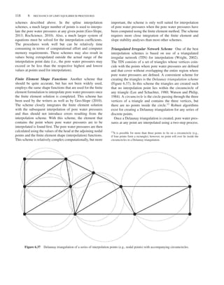
![Duncan c06.tex V3 - 07/21/2014 4:38 P.M. Page˜119
PORE WATER PRESSURE REPRESENTATION 119
First, the triangle that contains the point where pressures
are to be interpolated is located. Then, the pore water pres-
sures are interpolated linearly from the values of pore water
pressure at the three vertices of the enclosing triangle. The
interpolation equation is of the form of Eq. (6.110), but the
interpolation point never lies outside the perimeter of the tri-
angle formed by the three points used for interpolation. Also,
by using the Delaunay triangulation scheme, it is usually
possible to avoid having the three points used for interpo-
lation being located on essentially a straight line. One of
the most important advantages of the TIN-based scheme is
that algorithms exist for very quickly locating the appro-
priate triangle that contains the point where pressures are
to be interpolated, and, thus, the points to be used for in-
terpolation are located quickly (Lee and Schachter, 1980;
Mirante and Weingarten, 1982; Jones, 1990). In contrast, the
three- and four-point schemes described earlier, as well as
schemes using the finite element shape functions, may in-
volve a significant amount of time being spent on locating
the appropriate points or finite element that are to be used
for the interpolation. The TIN-based scheme also has the ad-
vantage of using a very simple linear interpolation function
[Eq. (6.110)] that requires very little computational time and
computer memory for storage.
Another advantage of the TIN-based interpolation scheme
is that it is applicable to interpolation using any type of irreg-
ularly gridded data, not just the results from finite element
analyses. For example, there may be cases where some pore
water pressures are recorded in piezometers or by ground-
water observations. These measured data may then be sup-
plemented by additional data points based on judgment and
interpretation to provide a grid of values. Such values can
then easily be used to compute values of pore water pressure
at other points using the TIN-based interpolation scheme.
Once any of these procedures is implemented in computer
codes, they can also be used for other forms of interpola-
tion required in slope stability computations. For example,
they are useful for interpolating values of undrained shear
strength when the undrained shear strengths vary both verti-
cally and horizontally. Conditions where such variation of
undrained shear strength occurs include mine tailings dis-
posal structures and clay foundations beneath embankments.
6.13.4 Phreatic Surface
Establishing variations of pore water pressure in two di-
mensions can be complex and time consuming. Considering
that groundwater and seepage conditions are often not well
known, approximations may be justified. In these cases, it
may be appropriate to use pore water pressures based on
the position of the phreatic surface. The phreatic surface is
the line of zero pressure (atmospheric pressure) at the upper
boundary of the seepage region.
Pore water pressure is equal to the product of the pressure
head at the point in question, hp, and the unit weight of
water, 𝛾w:
u = hp𝛾w (6.111)
If the phreatic surface is a straight line and the equipotential
lines are also straight lines (Figure 6.38a), perpendicular
to the phreatic surface, the pressure head is related to the
vertical distance, zp, below the phreatic surface by
hp = zp cos2
𝛽 (6.112)
where 𝛽 is the slope of the phreatic surface. If, instead, the
phreatic surface and equipotential lines are curved as shown
in Figure 6.38b, the pore water pressure can be expressed by
the following inequalities:
zp𝛾w cos2
𝛽′
< u < zp𝛾w cos2
𝛽′′
(6.113)
where 𝛽′ is the slope of the phreatic surface at the point where
the equipotential line intersects the phreatic surface, and 𝛽′′
is the slope of the phreatic surface directly above the point
of interest. In this case (𝛽′′ < 𝛽′), and it is conservative to
express the pore water pressure as
u = zp𝛾w cos2
𝛽′′
(6.114)
(a)
(b)
βʺ
βʹ
Phreatic surface
Equipotential (h = constant) line
P
zp
β
β
Phreatic surface
Equipotential (h = constant) line
hp
P
zp
z
p
c
o
s
β
Figure 6.38 (a) Linear and (b) curved phreatic surfaces used to
approximate pore water pressures.](https://image.slidesharecdn.com/soilstrengthandslopestability-220624112511-a82802bd/85/Soil-Strength-and-Slope-Stability-pdf-135-320.jpg)
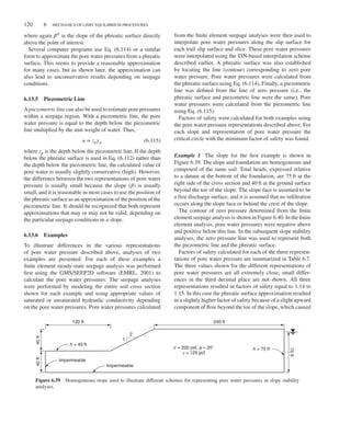


![126 7 METHODS OF ANALYZING SLOPE STABILITY
where 𝛾 is the unit weight of the soil in the embankment;
𝛾H represents the maximum vertical stress produced by the
embankment. Equation (7.8) is an equilibrium equation cor-
responding to ultimate conditions, that is, with the shear
strength of the soil fully mobilized. If, instead, only some
fraction of the shear strength is developed, that is, the factor
of safety is greater than unity, a factor of safety can be intro-
duced into the equilibrium equation (7.8) and we can write
𝛾H = 5.53
c
F
(7.9)
In this equation F is the factor of safety with respect to the
shear strength of the foundation, and the term c∕F represents
the mobilizes cohesion, cd. Equation (7.9) can be rearranged
to give
F = 5.53
c
𝛾H
(7.10)
Equation (7.10) can be used to estimate the factor of safety
against a deep-seated failure of an embankment on soft clay.
Equation (7.10) gives a conservative estimate of the factor
of safety of an embankment because it ignores the strength of
the embankment and the depth of the foundation in compar-
ison with the embankment width. Alternative bearing capac-
ity equations that are applicable to reinforced embankments
on thin clay foundations are presented in Chapter 8.
7.1.3 Infinite Slope
In Chapter 6, the equations for an infinite slope were pre-
sented. For these equations to be applicable, the depth of
the slip surface must be small compared to the lateral ex-
tent of the slope. However, in the case of cohesionless soils,
the factor of safety does not depend on the depth of the slip
surface. It is possible for a slip surface to form at a small
enough depth that the requirements for an infinite slope are
met, regardless of the lateral extent of the slope. Therefore, an
infinite slope analysis is rigorous and valid for cohesionless
slopes. The infinite slope analysis procedure is also applica-
ble to cases where there is a stronger layer of soil parallel
to the slope at shallow depth, for example, where a layer
of relatively weak weathered soil is underlain by stronger,
unweathered material.
The general equation for the factor of safety for an infinite
slope with the shear strength expressed in terms of total
stresses is
F = cot 𝛽 tan 𝜙 + (cot 𝛽 + tan 𝛽)
c
𝛾z
(7.11)
where z is the vertical depth of the slip surface below the
face of the slope. For shear strengths expressed by effective
stresses the equation for the factor of safety can be written as
F =
[
cot 𝛽 −
u
𝛾z
(cot 𝛽 + tan 𝛽)
]
tan 𝜙′
+ (cot 𝛽 + tan 𝛽)
c′
𝛾z
(7.12)
where u is the pore water pressure at the depth of the slip
surface.
For effective stress analyses, Eq. (7.12) can also be written
as
F = [cot 𝛽 − ru(cot 𝛽 + tan 𝛽)] tan 𝜙′
+ (cot 𝛽 + tan 𝛽)
c′
𝛾z
(7.13)
where ru is the pore pressure ratio defined by Bishop and
Morgenstern (1960) as
ru =
u
𝛾z
(7.14)
Values of ru can be determined for specific seepage condi-
tions. For example, for seepage parallel to the slope, the pore
pressure ratio, ru, is given by
ru =
𝛾w
𝛾
hw
z
cos2
𝛽 (7.15)
where hw is the height of the free water surface vertically
above the slip surface (Figure 7.2a). If seepage exits the slope
face at an angle (Figure 7.2b), the value of ru is given by
ru =
𝛾w
𝛾
1
1 + tan 𝛽 tan 𝜃
(7.16)
where 𝜃 is the angle between the direction of seepage (flow
lines) and horizontal. For the special case of horizontal seep-
age (𝜃 = 0), the expression for ru reduces to
ru =
𝛾w
𝛾
(7.17)
Recapitulation
• Simple equations can be used to compute the factor
of safety for several slope and shear strength con-
ditions, including a vertical slope in cohesive soil,
an embankment on a deep deposit of saturated clay,
and an infinite slope.
• Depending on the particular slope conditions and
equations used, the accuracy ranges from excellent,
(e.g., for a homogeneous slope in cohesionless soil)
to relatively imprecise (e.g., for bearing capacity of
an embankment on saturated clay).
7.2 SLOPE STABILITY CHARTS
The stability of homogeneous slopes can be analyzed us-
ing slope stability charts as described in Chapter 6. Fellenius
(1936) was one of the first to recognize that factors of safety
could be expressed by charts. His work was followed by the
work of Taylor (1937) and Janbu (1954b). Since the pioneer-
ing work of these authors, numerous others have developed
charts for slope stability. The charts developed by Janbu are](https://image.slidesharecdn.com/soilstrengthandslopestability-220624112511-a82802bd/85/Soil-Strength-and-Slope-Stability-pdf-142-320.jpg)
![SLOPE STABILITY CHARTS 127
z
hw
β
β θ
(a)
(b)
Figure 7.2 Infinite slope with seepage: (a) parallel to slope face and (b) exiting
the slope face.
some of the most useful for many conditions, and these are
described in further detail in Appendix A. The charts cover
a range in slope and soil conditions and they are quite easy
to use. In addition, the charts provide the minimum factor
of safety and eliminate the need to search for a critical slip
surface.
Stability charts rely on dimensionless relationships be-
tween the factor of safety and other parameters that describe
the slope geometry, soil shear strengths, and pore water pres-
sures. For example, the infinite slope equation for effective
stresses presented earlier [Eq. (7.13)] can be written as
F = [1 − ru(1 + tan2
𝛽)]
tan 𝜙′
tan 𝛽
+ (1 + tan2
𝛽)
c′
𝛾z
(7.18)
or
F = A
tan 𝜙′
tan 𝛽
+ B
c′
𝛾z
(7.19)
where
A = 1 − ru(1 + tan2
𝛽) (7.20)
B = 1 + tan2
𝛽 (7.21)
A and B are dimensionless parameters (stability numbers)
that depend only on the slope angle, and in the case of A,
the dimensionless pore water pressure coefficient, ru. Simple
charts for A and B as functions of the slope angle and pore
water pressure coefficient, ru, are presented in Appendix A.
For purely cohesive (𝜙 = 0) soils and homogeneous slopes,
the factor of safety can be expressed as
F = N0
c
𝛾H
(7.22)
where N0 is a stability number that depends on the slope
angle, and in the case of slopes flatter than about 1:1, on
the depth of the foundation below the slope. For vertical
slopes the value of N0 according to the Swedish slip circle
method is 3.83. This value (3.83) is slightly less than the
value of 4 shown in Eq. (7.5) based on a plane slip surface.
In general, circular slip surfaces give a lower factor of safety
than a plane, especially for flat slopes. Therefore, circles are
generally used for analysis of most slopes in cohesive soils.
A complete set of charts for cohesive slopes of various incli-
nations and foundation depths is presented in Appendix A.
Procedures are also presented for using average shear
strengths with the charts when the shear strength varies.
For slopes with both cohesion and friction, additional
dimensionless parameters are introduced. Janbu (1954b)
showed that the factor of safety could be expressed as
F = Ncf
c′
𝛾H
(7.23)
where Ncf is a dimensionless stability number. The stabil-
ity number depends on the slope angle, 𝛽, the pore water
pressures, u, and the dimensionless parameter 𝜆c𝜙, which is
defined as
𝜆c𝜙 =
𝛾H tan 𝜙′
c′
(7.24)
Stability charts employing 𝜆c𝜙 and Eq. (7.23) to calculate the
factor of safety are presented in Appendix A. These charts
can be used for soils with cohesion and friction as well
as a variety of pore water pressure and external surcharge
conditions.](https://image.slidesharecdn.com/soilstrengthandslopestability-220624112511-a82802bd/85/Soil-Strength-and-Slope-Stability-pdf-143-320.jpg)
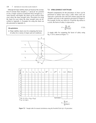
![FINITE ELEMENT ANALYSES OF SLOPE STABILITY 129
Slice
No.
1
b W
h1 cʹ u W cos α W sin α
W sin α
W
cos
α
-
u
Δℓ
cos
2
α
(W
cos
α
-
u
Δℓ
cos
2
α)tanϕʹ
u Δℓ cʹ Δℓ
ϕʹ
h2
γ1 h3
γ2 Δℓ α
γ3
2
3
4
5
6
7
8
9
10
Note: 1. W = b × (h1γ1 + h2γ2 + h3γ3)
2. Δℓ = b / cos α
Σ
Σ (W cos α – u Δℓ cos2
α) tan ϕʹ + cʹ Δℓ
F =
Summation:
Figure 7.4 Sample table for manual calculations using the Ordinary Method of Slices and effective stresses.
For the Ordinary Method of Slices with the shear strength
expressed in terms of effective stresses, the preferred
equation for computing the factor of safety is
F =
∑ [
c′Δ𝓁 +
(
W cos 𝛼 − uΔ𝓁 cos2𝛼
)
tan 𝜙′
]
∑
W sin 𝛼
(7.26)
A table for computing the factor of safety using this form
of the Ordinary Method of Slices equation is shown in
Figure 7.4.
Tables such as the ones shown in Figures 7.3 and 7.4 are
readily represented and implemented in computer spread-
sheet software. More sophisticated spreadsheets have been
developed for computing the factor of safety using proce-
dures of slices such as the Simplified Bishop, force equi-
librium, and even Chen and Morgenstern’s procedures (Low
et al., 1998, 2007; Low, 2003; Low and Tang, 2007; Low and
Duncan, 2013).
The number of different computer spreadsheets that have
been developed and used to compute factors of safety is
undoubtedly very large. This attests to the usefulness of
spreadsheets for slope stability analyses but at the same time
presents several important problems: First, because such a
large number of different spreadsheets are used and because
each spreadsheet is often used only once or twice, it is dif-
ficult to validate the correctness of spreadsheets. Also, be-
cause one person may write a spreadsheet, use it for some
computations, and then discard the spreadsheet, results are
sometimes poorly archived and difficult to interpret or to un-
derstand later. Electronic copies of the spreadsheet may have
been discarded. Hard copies of numerical tabulations from
the spreadsheet may have been saved, but unless the under-
lying equations, formulas, and logic that were used to create
the numerical values are also clearly documented, it may be
difficult to resolve inconsistencies or check for errors.
Recapitulation
• Spreadsheets provide a useful way of performing
calculations by the procedures of slices.
• Spreadsheet calculations can be difficult to check
and archive.
7.4 FINITE ELEMENT ANALYSES OF SLOPE
STABILITY
The finite element method has found increasing use in
geotechnical engineering practice over the past 50 years.
It was first used to solve problems of heat flow and water flow
in soils and later was applied to determination of stresses and
deformations in excavated slopes and embankments. More
recently, it has been used to calculate the factor of safety
defined in the same way as that used in limit equilibrium](https://image.slidesharecdn.com/soilstrengthandslopestability-220624112511-a82802bd/85/Soil-Strength-and-Slope-Stability-pdf-145-320.jpg)


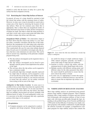


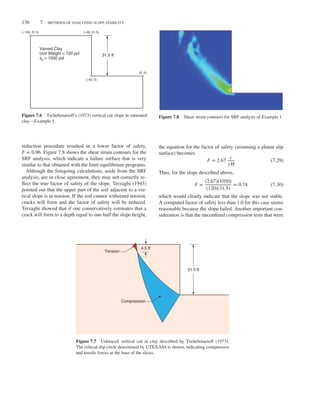


![EXAMPLES FOR VERIFICATION OF STABILITY COMPUTATIONS 143
100 ft
100 ft
Critical circle -
Spencer’s
procedure
50 ft
r = 174 ft
(‒600, 0)
(‒600, ‒50) (100,‒50)
(‒300, 100)
(‒100, 124)
(‒200, 100)
(‒500, 0) (100, 0)
(0, 0)
1 1
2 Sand:
Saturated clay: su = 2500 psf (ϕ = 0)
γ = 140 pcf
c = 0
ϕ = 40°
γ = 40 pcf
2
Figure 7.18 Cohesionless fill slope on saturated clay foundation.
with time and its strength is expected to increase with time.
Therefore, the critical period (lowest factor of safety) for the
embankment is immediately after construction. Although
some amount of drainage and consolidation may occur while
the embankment is being constructed, it is conservative to
ignore this factor, and to use undrained strengths from UU
tests performed on undisturbed samples of the foundation
clay taken before construction.
Soil shear strength and unit weight properties are shown in
Figure 7.18. Drained (effective stress) shear strength parame-
ters are shown for the sand embankment, and undrained shear
strengths are shown for the clay foundation. Stability com-
putations were performed using limit equilibrium computer
programs and several procedures of slices.
The minimum factors of safety for various procedures
are summarized in Table 7.5, and the critical slip surface
by Spencer’s procedure using UTEXAS4 is shown in
Figure 7.18. Contours of shear strain for the SRF analysis
are shown in Figure 7.19 for comparison. Since the cross
section is symmetrical, the SRF analysis indicates that
failure can occur in either direction. The SRF analysis gave
a factor of safety equal to 1.19, essentially the same as the
limit equilibrium analyses.
As expected, the Simplified Bishop procedure gives a value
for the factor of safety that is very close to the one calcu-
lated by Spencer’s procedure. The Simplified Janbu proce-
dure without the correction factor applied gives a factor of
safety that is approximately 10 percent lower, but the cor-
rected value (1.16) agrees closely with the values by the
Simplified Bishop and Spencer’s procedures. The factor of
safety determined using the SRF approach agreed well with
the results from Spencer’s procedure for all programs.
The factor of safety was also computed using the Ordinary
Method of Slices with a spreadsheet program for the critical
circle found by Spencer’s procedure. The computations are
shown in Figure 7.20. The computed factor of safety is 1.08,
approximately 10 percent less than the value calculated using
Spencer’s procedure. Differences of this order (10 percent)
are typical for cases like this because, with 𝜙 > 0, shear
Table 7.5 Summary of Slope Stability Analyses for a
Cohesionless Embankment Supported by a Saturated
Clay Foundation
Factor of Safety
Procedure UTEXAS4 SLOPE/W SLIDE Phase2
Spencer 1.19 1.20 1.20 —
Simplified Bishop 1.22 1.22 1.23 —
Simplified
Janbu—no
correction
1.07 1.07 1.08 —
Simplified
Janbu—with
correction, f0
1.16a 1.16a 1.17 —
Strength reduction
factor
— — — 1.19
a
Correction based on Figure 6.13 for d∕L = 0.34; f0 = 1.09.
strength varies with normal stress, and the normal stresses
on the bases of slices from the Ordinary Method of Slices
are too low.
As an additional, approximate check on the calculations,
the bearing capacity equation [Eq. (7.10)] was used to calcu-
late a factor of safety. This gave
F = 5.53
2500
(140)(100)
= 0.99 (7.32)
The bearing capacity factor in Eq. (5.32) is based on a foun-
dation of unlimited depth and is conservative for this case
where the failure mechanism is affected by the limited depth
of clay in the foundation. Although the bearing capacity so-
lution represented by Eq. (7.32) underestimates the stabil-
ity of the embankment in this example, it provides a simple
and convenient way of preliminary screening for potential
problems. In general, if the factor of safety for bearing ca-
pacity is near or below 1.0, the factor of safety is likely to be
marginal and additional, more detailed analyses are probably
warranted.](https://image.slidesharecdn.com/soilstrengthandslopestability-220624112511-a82802bd/85/Soil-Strength-and-Slope-Stability-pdf-159-320.jpg)


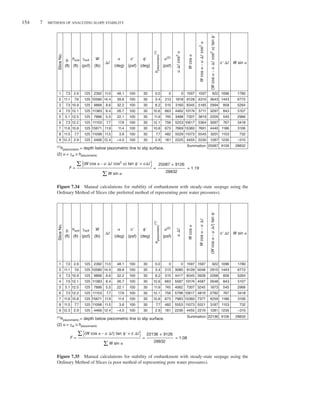
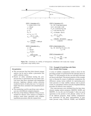

![EXAMPLES FOR VERIFICATION OF STABILITY COMPUTATIONS 157
Shell
Shell
Core
Figure 7.39 Contours of shear strain determined from SRF analysis for Example 8. The pore pressures were determined from a finite
element seepage analysis.
W 1.8
1.6
1.8
1.6
Trial F
Solution:
F = 1.61
Calculated
F
1.4
1.4
(lb)
W
(lb)
α
(deg)
W
sin
α
b
(ft)
1
2
3
4
5
6
7
8
9
10
1
2
3
4
5
6
7
8
9
10
36659
215174
683527
894190
1406585
1648280
315386
1055716
867907
98993
43.2
40.2
35.0
28.7
21.7
13.1
7.7
3.4
–4.8
–11.7
(a)
(b)
(c)
20.0
35.2
65.0
62.5
89.9
105.7
21.2
81.8
114.7
49.8
13.1
20.8
10.0
29.5
52.5
82.2
101.4
92.2
54.1
14.2
140
140
140
140
140
140
140
140
140
140
120
120
120
120
120
120
120
120
120
120
36659
215174
683527
894190
1406585
1648280
315386
1055716
867907
98993
0.0
26.6
76.0
84.9
69.1
34.2
5.6
0.0
0.0
0.0
Slice
No.
Slice
No.
Trial F = 1.4 Trial F = 1.6 Trial F = 1.8
h
shell
(ft)
h
core
(ft)
(1) hpiezometric = depth below piezometric line to slip surface.
h
piezometric
(1)
u
(2)
(psf)
F1 = = 1.603
(2) u = γw × hpiezometric.
γ
shell
(ft)
γ
core
(pcf)
25.110
138831
391572
429214
519784
374514
42435
62854
–72569
–20099
0
0
0
0
0
0
0
0
0
0
38
20
20
20
20
20
20
38
38
38
0.0
23.2
38.3
55.3
59.9
34.2
11.5
12.9
7.2
0.0
0
1450
2392
3449
3741
2131
719
805
452
0
28641
59724
192187
247055
389600
517970
109240
773349
637567
77342
1.11
0.93
0.97
1.00
1.03
1.03
1.03
1.03
0.95
0.87
Sum:
Sum: Sum: Sum:
3033119
3033119
1891646
1891646 3049608 3062944
28641
59724
192187
247055
389600
517970
109240
773349
671239
77342
1.06
0.91
0.95
0.99
1.01
1.03
1.02
1.03
0.96
0.88
26942
65575
202309
250447
384494
505074
106939
752799
667142
87886
1.03
0.89
0.94
0.97
1.00
1.02
1.02
1.02
0.96
0.89
27918
666770
205441
253565
388071
507919
107296
755174
663990
86799
F = F
Σ mα
m
α
m
α
m
α
mα = cos α +
ΣW sin α
cʹb + (W – ub) tan ϕʹ
cʹb
+
(W
–
ub)
tan
ϕʹ
[c
ʹ
b
+
(W
–
ub)
tan
ϕʹ]
÷
m
α
[c
ʹ
b
+
(W
–
ub)
tan
ϕʹ]
÷
m
α
[c
ʹ
b
+
(W
–
ub)
tan
ϕʹ]
÷
m
α
ϕʹ
(deg)
cʹ
(psf)
F2 = = 1.612
3049608
1891646
F3 = = 1.619
3062944
1891646
sin α tan ϕʹ
Figure 7.40 Manual calculations for stability of clay core dam with steady-state seepage using
the Simplified Bishop procedure: (a) calculation of slice weights, (b) calculations for factor of
safety, and (c) summary of trial-and-error solution for F.](https://image.slidesharecdn.com/soilstrengthandslopestability-220624112511-a82802bd/85/Soil-Strength-and-Slope-Stability-pdf-173-320.jpg)


![REINFORCEMENT FORCES 161
knitted from polyester fibers. Galvanized or epoxy-coated
steel strips have been used for slope reinforcement. The strips
usually have raised ribs to increase their pullout resistance.
Polyester yarns can be coextruded with polyethylene sheaths
to create geosynthetic strips. Welded mild steel mats or grids
have also been used for reinforcing slopes and embankments.
Key sources of information about geosynthetic reinforcing
for slopes are the book by Koerner (2012), which contains a
great deal of information on the fundamental characteristics
and properties of polymers, geotextiles, and geogrids, and
the FHWA (2009) publication, which covers a wide range of
subjects related to geotextiles, geogrids, steel strips, and steel
grids, and their use in reinforced walls and slopes.
8.4 REINFORCEMENT FORCES
The long-term capacity of reinforcement, denoted here as
TLTDS, depends on the following factors:
• Tensile strength. For steel, the tensile strength is the
yield strength. For geotextiles, the tensile strength is
normally measured using short-term wide-width tensile
tests (ASTM D4594, 2009). Geogrids are often tensile
tested using the single rib or multirib methods described
in ASTM D6637 (2011).
• Creep characteristics. Steel does not creep appreciably,
but geosynthetic materials do. The tensile loads used
for design of geotextile- and geogrid-reinforced walls
must be reduced to values lower than those measured in
short-term tensile tests, to stresses that are low enough
so that little or no creep deformation will occur over the
design life of the structure.
• Installation damage. Geogrids and geotextiles are sub-
ject to damage during installation that results in holes
and tears. Polyvinylchloride (PVC) or another func-
tionally equivalent polymeric materials are used to coat
polyethylene terephthalate (PET) geogrids to increase
the resistance to installation damage. Geotextiles used
as reinforcement are not coated. In both cases, instal-
lation damage testing should be performed to quan-
tify the potential for damage. Steel reinforcement is
not typically susceptible to damage during installation.
However, if the steel has an epoxy or PVC coating for
corrosion protection, the coating may be adversely af-
fected. For this reason, steel reinforcement is usually
galvanized.
• Durability. The mechanical properties of geosynthetics
are subject to deterioration during service as a result
of attack by chemical and biological agents. Steel is
subject to corrosion.
• Pullout resistance. Near the ends of the reinforcement,
capacity is limited by the resistance to pullout, or slip
between the reinforcement and the soil within which it
is embedded.
• Reinforcement stiffness and tolerable strain within the
slope. To be useful for slope reinforcement, the reinforc-
ing material must have stiffness as well as strength. A
very strong but easily extensible rubber band would not
provide effective reinforcement because it would have
to stretch so much to mobilize its tensile capacity that it
would not be able to limit the deformation of the slope.
Values of TLTDS, the long-term capacity of reinforcing
materials, must satisfy the following criteria:
1. TLTDS ≤ capacity determined by short-term tensile
strength, creep, installation damage, and deterioration
of properties over time.
2. TLTDS ≤ capacity determined by pullout resistance.
Methods of applying these requirements to geosynthetics
and steel reinforcing are described in the following sections.
8.4.1 Criterion 1: Creep, Installation Damage,
and Deterioration in Properties over Time
Geotextiles and Geogrids The effects of creep, installation
damage, and long-term deterioration on geosynthetic mate-
rials can be evaluated using the expression
TLTDS =
Tult
(RFCR)(RFID)(RFD)
(8.5)
where TLTDS is the long-term design strength (F/L); Tult is
the short-term ultimate strength, measured in a wide-strip
tension test or a rib tensile test (F/L); RFCR is the strength
reduction factor to allow for creep under long-term load;
RFID is the strength reduction factor to allow for installation
damage; and RFD is the strength reduction factor to allow
for deterioration in service. Values of RFCR, RFID, and RFD
recommended by the FHWA are given in Table 8.1. The units
of TLTDS and Tult are force per unit length of reinforced slope.
Steel Reinforcement Steel reinforcing does not creep
appreciably and is not subject to significant installation
damage. Epoxy and PVC coatings are subject to installation
damage, but galvanized coating is not. The effects of
long-term deterioration of steel due to corrosion can be
evaluated using the expression
TLTDS ≤ Ac fy (8.6)
where TLTDS is the allowable long-term reinforcement
design strength (F/L); Ac is the cross-sectional area of
reinforcement after corrosion, calculated by reducing the
metal thickness by the loss expected during the life of the
installation [Ac is the area per unit length of slope (L2∕L)];](https://image.slidesharecdn.com/soilstrengthandslopestability-220624112511-a82802bd/85/Soil-Strength-and-Slope-Stability-pdf-177-320.jpg)
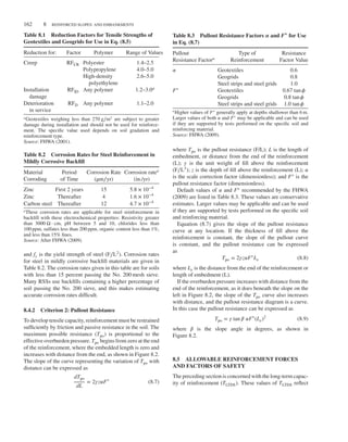


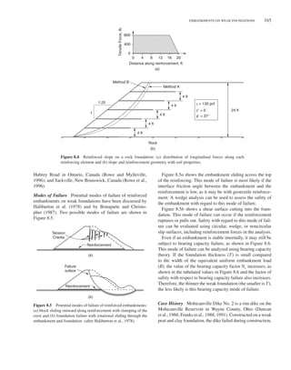


![Duncan c09.tex V2 - 06/20/2014 3:12 P.M. Page˜170
170 9 ANALYSES FOR RAPID DRAWDOWN
soils are readily determined by means of isotropically
consolidated–undrained (ICU) triaxial compression tests
with pore pressure measurements. This type of test is well
within the capability of most soil mechanics laboratories.
The disadvantage of effective stress analyses is that it is
difficult to estimate the pore water pressures that will ex-
ist within low-permeability soils during drawdown. The pore
pressure changes during drawdown depend on the changes in
stress that result from the changing water loads on the slope
and the undrained response of the soils within the slope to
these changes in load. While the changes in stress can be
estimated with reasonable accuracy, particularly at shallow
depths beneath the surface of the slope, the undrained re-
sponse of the soil is much harder to estimate. The changes
in pore pressure are considerably different for materials that
tend to dilate during shear and those that do not. Although in
principle it is possible to estimate these pore water pressures,
for example, by using Skempton’s pore water pressure coef-
ficients (Skempton, 1954), in practice this is difficult and the
results are uncertain.
Most effective stress analyses of stability during rapid
drawdown have used the assumptions regarding pore water
pressures that were suggested by Bishop (1954) and later
used by Morgenstern (1963). These assumptions have been
justified on the basis of the fact that they are conservative
in most cases. They have been found to result in reason-
able values of factor of safety for dams that suffered rapid
drawdown failures: Wong et al. (1983) found that the val-
ues of safety factor calculated using Morgenstern’s assump-
tion were F = 1.2 for Pilarcitos Dam and F = 1.0 for Walter
Bouldin Dam, both of which failed.
It seems likely that Bishop and Morgenstern’s assumptions
for pore water pressures during drawdown are more accurate
for soils that do not tend to dilate during shear than for those
that do tend to dilate. Thus, although these assumptions may
show reasonable correspondence with failures of slopes in
materials that are not densely compacted and that tend to con-
tract during shear, they are likely to be unduly conservative
for better-compacted materials that do tend to dilate during
shear. Use of effective stress analyses based on the Bishop
and Morgenstern assumptions would treat all fill materials
alike with respect to pore water pressures during drawdown,
regardless of how well they are compacted or how strongly
they might tend to dilate during shear.
Terzaghi and Peck (1967) suggested that pore water pres-
sures during drawdown in well-compacted silty sands could
be estimated using flow nets. Several investigators (Browzin,
1961; Brahma and Harr, 1963; Newlin and Rossier, 1967;
Desai and Sherman, 1971; Desai, 1972, 1977) used theoret-
ical methods to analyze the nonsteady flow conditions fol-
lowing drawdown. Like the Bishop and Morgenstern pore
pressure assumptions, these methods do not consider the
behavior of the soil with regard to dilatancy and are thus not
capable of representing the important factors that control the
pore water pressures during drawdown.
Svano and Nordal (1987) and Wright and Duncan (1987)
used procedures for estimating pore water pressures dur-
ing drawdown that reflect the influence of dilatancy on the
pore water pressure changes. Svano and Nordal (1987) used
two-stage stability analyses and iterated to achieve consis-
tency between the calculated factor of safety and the values
of the pore water pressures. Wright and Duncan (1987) used
finite element analyses to estimate the stress changes during
drawdown and Skempton’s pore pressure parameters to cal-
culate the pore water pressures. These studies indicate that it
is possible to estimate realistic pore water pressures for effec-
tive stress analyses, but it is more cumbersome and difficult
than using total stress analyses, as described in the following
sections.
Terzaghi and Peck (1967) summarized the problems
in estimating pore water pressures during drawdown in
these words:
[I]n order to determine the pore pressure conditions for the
drawdown state, all the following factors need to be known: The
location of the boundaries between materials with significantly
different properties; the permeability and consolidation charac-
teristics of each of these materials; and the anticipated maxi-
mum rate of drawdown. In addition, the pore pressures induced
by the changes in the shearing stresses themselves … need to be
taken into consideration. In engineering practice, few of these
factors can be reliably determined. The gaps in the available in-
formation must be filled by the most unfavorable assumptions
compatible with the known facts.
By using undrained strengths in low-permeability zones,
as described in the following sections, many of the prob-
lems associated with estimating pore water pressures for
effective stress analyses can be avoided, and the accuracy
of rapid drawdown stability analyses can be improved very
considerably.
9.2.2 Total Stress Methods
Total stress methods are based on undrained shear strengths
in low-permeability zones. The undrained shear strengths
are estimated based on the effective stresses that exist in
the slope prior to drawdown. Some zones within the slope
may consolidate with time following construction, and their
undrained strengths will increase. Portions of the same soils
at lower stresses (near the surface of the slope) may expand
following construction, and their undrained strengths will
decrease with time.
Several total stress analysis methods have been suggested
and used for sudden-drawdown analyses. These include
the U.S. Army Corps of Engineer’s (1970) method and](https://image.slidesharecdn.com/soilstrengthandslopestability-220624112511-a82802bd/85/Soil-Strength-and-Slope-Stability-pdf-186-320.jpg)
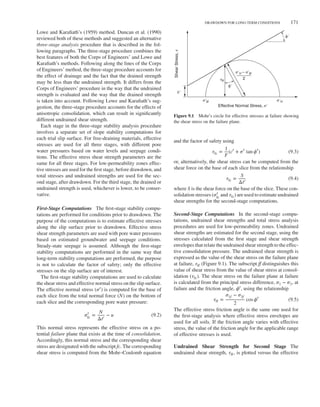

![Duncan c09.tex V2 - 06/20/2014 3:12 P.M. Page˜173
DRAWDOWN FOR LONG-TERM CONDITIONS 173
Variation of 𝛕ff with 𝛔′
fc
and Kc The undrained shear
strength envelopes shown in Figure 9.2, for Kc = 1 and
Kc = Kf , represent the extremes possible for the lowest and
highest possible values of Kc. Lowe and Karafiath (1959)
showed that for the same value of 𝜎′
fc
, the undrained strength
(𝜏ff) varies with the value of Kc. They recommended that
anisotropically consolidated undrained (ACU) triaxial tests
be performed to measure undrained shear strengths using
a range of Kc values to develop data that could be used
to evaluate undrained strengths for second-stage analyses.
This procedure results in accurate evaluation of undrained
strengths for the second-stage analyses but requires exten-
sive and difficult testing. The ACU test specimens must be
consolidated slowly to avoid failure during consolidation.
Wong et al. (1983) found that the difficult ACU tests
could be avoided by interpolating undrained strengths for
values of Kc between Kc = 1 and Kc = Kf instead of deter-
mining the strengths experimentally. They found that val-
ues of 𝜏ff calculated assuming that 𝜏ff varies linearly with
Kc were the very nearly same as values measured in ACU
tests. Using this method of interpolation, only isotropically
consolidated–undrained (ICU) tests with pore water pres-
sure measurements need be performed. Both of the envelopes
shown in Figure 9.2 can be determined from ICU tests, which
are much easier to perform than ACU tests.
Once the Kc = Kf and Kc = 1 envelopes shown in
Figure 9.2 have been determined, the undrained shear
strength for the second-stage computations is obtained
based on the effective normal stress on the slip surface, 𝜎′
fc
[Eq. (9.2)] and the estimated effective principal stress ratio
for consolidation, Kc. The effective principal stress ratio for
consolidation is estimated following the recommendations of
Lowe and Karafiath (1959). They suggested the assumption
that the orientation of the principal stresses at consolidation
is the same as the orientation of the principal stresses at
failure. This leads to the following equation for the effective
principal stress ratio:
K1 =
𝜎′
fc
+ 𝜏fc[(sin 𝜙′ + 1)∕ cos 𝜙′]
𝜎′
fc
+ 𝜏fc[(sin 𝜙′ − 1)∕ cos 𝜙′]
(9.10)
where K1 is the effective principal stress ratio for consolida-
tion corresponding to the stage 1 analyses and 𝜎′
fc
and 𝜏fc are
the effective normal stress and shear stress on the shear plane
at consolidation.
Values of the effective principal stress ratio can be cal-
culated from Eq. (9.10) using the shear stress and effective
normal stress calculated from Eqs. (9.2) and (9.3); the fric-
tion angle is the effective stress friction angle used in the
first-stage computations and in Eq. (9.5) to calculate 𝜏ff. Val-
ues of the undrained shear strength for the effective consoli-
dation pressure, 𝜎′
fc
, and a consolidation stress ratio Kc = K1,
are obtained from the two shear strength envelopes shown
in Figure 9.2. Linear interpolation between the values for
Kc = 1 and Kc = Kf to obtain the value corresponding to K1
can be expressed by
𝜏ff =
(Kf − K1)𝜏ff(Kc=1) + (K1 − 1)𝜏ff(Kc=Kf )
Kf − 1
(9.11)
where 𝜏ff(Kc=1) and 𝜏ff(Kc=Kf ) are the undrained shear
strengths from the two shear strength envelopes shown in
Figure 9.2. The undrained shear strengths are determined
from these two envelopes using the value of the effective
stress, 𝜎′
fc
, which was calculated from Eq. (9.2).
The effective principal stress ratio at failure shown in
Eq. (9.11) can be calculated from the effective stress shear
strength parameters. If there is no cohesion, the value for Kf
does not depend on the magnitude of the stress and is given
by
Kf = tan2
(
45 +
𝜙′
2
)
(9.12)
If the value of c′ is not zero, the value of Kf depends on the
effective stress on the slip surface and is given by
Kf =
(𝜎′ + c′ cos 𝜙′)(1 + sin 𝜙′)
(𝜎′ − c′ cos 𝜙′)(1 − sin 𝜙′)
(9.13)
where 𝜎′ is the effective stress on the slip surface after con-
solidation (and also at failure because Kc = Kf ).
If a significant effective cohesion (c′) exists, the effective
minor principal stress, 𝜎′
3
implicit in Eqs. (9.10) and (9.13)
may become negative (i.e., the terms in the denominator of
these equations become negative). When this occurs, the ef-
fective consolidation stress ratios become negative and are
nonsensical. The negative stress results from the fact that the
soil is assumed to have cohesion, and this implies a tensile
strength. The corresponding negative values for 𝜎′
3
are, how-
ever, not realistic. In cases where negative effective stresses
are calculated, the values are rejected and instead of interpo-
lating shear strengths using values of Kc, the shear strength is
taken to be the lower of the shear strengths from the Kc = 1
and Kc = Kf envelopes. Negative effective stresses can be de-
tected by calculating the effective minor principal stresses
after consolidation using Eqs. (9.14) and (9.15):
𝜎′
3c = 𝜎′
fc + 𝜏fc
sin 𝜙′ − 1
cos 𝜙′
(9.14)
𝜎′
3f = (𝜎′
fc − c′
cos 𝜙′
)
1 − sin 𝜙′
cos2𝜙′
(9.15)
Equation (9.14) is the effective minor principal stress corre-
sponding to the Kc = 1 envelope; Eq. (9.15) corresponds to
the Kc = Kf envelope. The values of 𝜎′
3c
and 𝜎′
3f
correspond
to the stresses in Eqs. (9.10) and (9.13), respectively. If either
value is negative (or zero), no interpolation is performed and
the lower of the Kc = 1 and Kc = Kf strengths is used for the
undrained shear strength in the second-stage stability com-
putations. After the undrained shear strength is determined
for each slice, a total stress analysis is performed using the](https://image.slidesharecdn.com/soilstrengthandslopestability-220624112511-a82802bd/85/Soil-Strength-and-Slope-Stability-pdf-189-320.jpg)

![Duncan c09.tex V2 - 06/20/2014 3:12 P.M. Page˜175
DRAWDOWN FOR LONG-TERM CONDITIONS 175
0
0
2000
4000
40°
20°
6000 Kc = Kf Kc = 1
2000 4000 6000
σʹfc, psf
τ
ff
,
psf
8000 10000
Figure 9.5 Shear strength envelopes for example problem.
water depth has no effect on the final results as long as the
slope is fully submerged before drawdown. The total (satu-
rated) unit weight of the soil is 125 pcf. The effective stress
shear strength parameters are c′ = 0, 𝜙′ = 40 degrees. The
intercept and slope of the Kc = 1 undrained shear strength
envelope (d and 𝜓) are 2000 psf and 20 degrees. The shear
strength envelopes are shown in Figure 9.5.
Stability calculations are performed for two slip surfaces.
Both of the slip surfaces are planes parallel to the sur-
face of the slope; one is 5 ft deep, the other is 30 ft deep.
Total drawdown is assumed to occur (i.e., the water is as-
sumed to be fully removed from the face of the slope).
It is further assumed that after drainage has occurred, the
pore water pressures are zero. The calculations for each of
the three stages are described below, and key quantities are
summarized in Table 9.2.
First-Stage Analysis The total normal stress on the slip
surface is computed for a submerged infinite slope from the
equation
𝜎 = 𝛾zcos2
𝛽 + 𝛾w(hw + zsin2
𝛽) (9.18)
Thus, for the slip surface at a depth of 5 ft,
𝜎 = (125)(5)cos2
(18.4∘) + (62.4)[100 + (5)sin2
(18.4∘)]
= 6834 psf (9.19)
Similarly, for the slip surface at a depth of 30 ft, the total
normal stress is 9803 psf. The pore water pressure on the
slip plane is computed from
u = 𝛾w(z + hw) (9.20)
For the slip surface at a depth of 5 ft, the pore water pressure
is
u = (62.4)(5 + 100) = 6552 psf (9.21)
and, similarly, the pore water pressure at a depth of 30 ft
is u = 8112 psf. The effective normal stress is computed by
subtracting the pore water pressure from the total stress (i.e.,
𝜎′ = 𝜎 − u). Thus, for the slip surface at a depth of 5 ft the
effective stress is
𝜎′
= 6834 − 6552 = 282 psf (9.22)
Table 9.2 Summary of Stability Calculations for Rapid Drawdown of Example Slope
Quantity z = 5 ft z = 30 ft
Stage 1 Total normal stress on the failure plane, 𝜎fc 6834 psf 9803 psf
Pore water pressure, u 6552 psf 8112 psf
Effective normal stress on the failure plane (consolidation
pressure), 𝜎′
fc
282 psf 1691 psf
Shear stress on the failure plane after consolidation, 𝜏fc 94 psf 562 psf
Stage 2 Shear strength, 𝜏ff(Kc=1) 2103 psf 2615 psf
Shear strength, 𝜏ff(Kc=Kf ) 237 psf 1419 psf
Effective principal stress ratio for consolidation, K1 2.0 2.0
Undrained shear strength (interpolated), 𝜏ff 1585 psf 2283 psf
Shear stress (after drawdown), 𝜏 187 psf 1123 psf
Factor of safety (undrained strengths) 8.48 2.03
Stage 3 Total normal stress (after drawdown), 𝜎 563 psf 3376 psf
Pore water pressure (after drawdown and drainage) 0 0
Effective normal stress (after drawdown and drainage) 563 psf 3376 psf
Drained shear strength 472 psf 2833 psf
Final stage Governing strength after drawdown 472 psf (drained) 2283 psf (undrained)
Factor of safety after drawdown 2.52 (third stage) 2.03 (second stage)](https://image.slidesharecdn.com/soilstrengthandslopestability-220624112511-a82802bd/85/Soil-Strength-and-Slope-Stability-pdf-191-320.jpg)
![Duncan c09.tex V2 - 06/20/2014 3:12 P.M. Page˜176
176 9 ANALYSES FOR RAPID DRAWDOWN
and for the slip surface at a depth of 30 ft, the effective normal
stress is 1691 psf (= 9803 − 8112). These represent the ef-
fective normal stresses after consolidation, 𝜎′
fc
. The effective
normal stresses can also be calculated directly using sub-
merged unit weights (𝛾′) and the following equation because
there is no flow:
𝜎′
= 𝛾′
z cos2
𝛽 (9.23)
The shear stress on the slip surfaces is calculated from
𝜏 = (𝛾 − 𝛾w)z sin 𝛽 cos 𝛽 (9.24)
For the slip surface at a depth of 5 ft, this gives
𝜏 = (125 − 62.4)(5) sin(18.4∘) cos(18.4∘) = 94 psf (9.25)
and, similarly, for the slip surface at a depth of 30 ft the shear
stress is 562 psf. These stresses represent the shear stresses,
𝜏fc, on the two potential slip surfaces after consolidation. The
consolidation stresses are summarized in Table 9.2.
Second-Stage Analysis For the second-stage analysis the
undrained shear strengths are determined based on 𝜎′
fc
and
𝜏fc. The undrained shear strengths for the Kc = 1 shear
strength envelope are computed using the equation
𝜏ff(Kc=1) = d + 𝜎′
fc tan 𝜓 (9.26)
For the slip surface at a depth of 5 ft, this gives
𝜏ff(Kc=1) = 2000 + (282) tan (20∘) = 2103 psf (9.27)
The corresponding value for the slip surface at a depth of 30 ft
is 𝜏ff(Kc=1) = 2615 psf. The shear strengths from the envelope
for Kc = Kf are computed from
𝜏ff(Kc=Kf ) = c′
+ 𝜎′
fc tan 𝜙′
(9.28)
For the slip plane at a depth of 5 ft, this gives
𝜏ff(Kc=Kf ) = 0 + (252) tan (40∘) = 237 psf (9.29)
Similarly, for the slip surface at 30 ft depth, 𝜏ff(Kc=Kf ) is
1419 psf.
The undrained shear strengths for the second-stage analysis
are interpolated using the effective principal stress ratios
and the undrained shear strength values determined above.
The effective principal stress ratios after consolidation are
calculated using the stresses from the first-stage analysis and
Eq. (9.10). For the slip surface at a depth of 5 ft,
K1 =
282 + 94{[sin(40∘) + 1]∕cos(40∘)}
282 + 94{[sin(40∘) − 1]∕cos(40∘)}
= 2.0 (9.30)
The effective principal stress ratio for consolidation for the
slip surface at a depth of 30 ft is also equal to 2.0.
The effective principal stress ratio at failure is calculated
from Eq. (9.12). The effective principal stress ratio at fail-
ure is 4.6 and is the same for both depths because c′ = 0.
Undrained shear strengths are determined using Eq. (9.11).
For the slip surfaces at depths of 5 and 30 ft, the shear
strengths are as follows:
𝜏ff =
⎧
⎪
⎪
⎪
⎨
⎪
⎪
⎪
⎩
(4.6 − 2.0) 2103 + (2.0 − 1)237
4.6 − 1
= 1585 psf
for 5-ft depth
(4.6 − 2.0)2615 + (2.0 − 1)1419
4.6 − 1
= 2283 psf
for 30-ft depth
(9.31)
(9.32)
The next step in the second-stage analysis is to calculate
the factor of safety after drawdown using the undrained shear
strengths. For the infinite slope and complete drawdown (no
water above slope), the shear stress is calculated from
𝜏 = 𝛾z sin 𝛽 cos 𝛽 (9.33)
For the slip surface at a depth of 5 ft, this gives
𝜏 = (125)(5) sin(18.4∘) cos(18.4∘) = 187 psf (9.34)
Similarly, for the slip surface at a depth of 30 ft the shear
stress is 1123 psf. The factors of safety for the slip surfaces
are calculated by dividing the undrained shear strength by the
shear stress. For the slip surfaces at depths of 5 and 30 ft, this
gives, respectively,
F =
⎧
⎪
⎨
⎪
⎩
1585
187
= 8.48 for 5-ft depth
2283
1123
= 2.03 for 30-ft depth
(9.35)
(9.36)
These values represent the factors of safety for undrained
conditions during drawdown.
Third-Stage Analysis The third-stage analysis is begun
by estimating the fully drained shear strengths of the soil
(assuming that all excess pore water pressures due to draw-
down have dissipated). For this example the water level is
assumed to be lowered to such a depth that there will be
no pore water pressures after drainage is complete. The to-
tal normal stress and effective stress are equal since the pore
water pressures are zero. The effective stress for drained con-
ditions after drawdown is computed from the equation
𝜎′
= 𝛾z cos2
𝛽 (9.37)
For the slip surface at a depth of 5 ft, this gives
𝜎′
= (125)(5) cos2
(18.4∘) = 563 (9.38)
The drained shear strength is then
𝜏drained = 0 + (563) tan(40∘) = 472 psf (9.39)
This value (472 psf) is much less than the value of undrained
shear strength (1585 psf) determined earlier. Therefore,
the factor of safety would be lower if drainage occurred.](https://image.slidesharecdn.com/soilstrengthandslopestability-220624112511-a82802bd/85/Soil-Strength-and-Slope-Stability-pdf-192-320.jpg)
![Duncan c09.tex V2 - 06/20/2014 3:12 P.M. Page˜177
SHEAR-INDUCED PORE PRESSURE CHANGES 177
The shear stress was calculated above [Eq. (9.34)] to be 187
psf, and the factor of safety for the slip surface at a depth of
5 ft is, therefore,
F =
472
187
= 2.52 (9.40)
For the slip surface at a depth of 30 ft, the effective normal
stress after drainage is calculated as
𝜎′
= (125)(30) cos2
(18.4∘) = 3376 (9.41)
and the corresponding drained shear strength is
𝜏drained = 0 + (3376) tan(40∘) = 2833 (9.42)
This value of 2833 psf for the drained shear strength is
higher than the value of 2283 psf determined earlier for the
undrained shear strength. Thus, the undrained shear strength
controls, and the factor of safety is equal to the value of 2.02
that was calculated earlier [Eq. (9.36)].
The calculations for this example show that the drained
shear strength controls the stability after drawdown for the
shallow (5 ft) depth while the undrained shear strength con-
trols the stability for deeper (30 ft) depth. It is commonly
found that drained shear strength is smaller at shallower
depths, and undrained shear strength is smaller at deeper
depths. Generally, this pattern of drained and undrained shear
strengths controlling the stability is expected to happen.
For slip surfaces that encompass a range of depths, the con-
trolling shear strength may be the drained strength in some
parts and the undrained strength in others.
9.3 PARTIAL DRAINAGE
Partial drainage during drawdown may result in reduced pore
water pressures and improved stability. Theoretically, such
improvement in stability could be computed and taken into
account by effective stress stability analyses. The compu-
tations would be performed like effective stress analyses
for long-term stability except that pore water pressures for
drawdown would be considered. Although such an approach
seems logical, it is beyond the current state of practice and
probably beyond the present state of the art. The principal
difficulties lie in predicting the pore water pressures induced
by drawdown.
9.4 SHEAR-INDUCED PORE PRESSURE
CHANGES
Approaches based on construction of flow nets, and most nu-
merical solutions (finite difference, finite element), do not ac-
count for the very important changes in pore water pressures
that are induced by shear deformations. Well-compacted fills
are likely to tend to dilate during drawdown, reducing pore
pressures and increasing strength. Poorly compacted fills are
likely to tend to compress during drawdown, increasing pore
pressures and reducing strength. These effects are reflected in
total stress analyses of the type described above through the
very different undrained strengths used for well-compacted
and poorly compacted fill materials. Ignoring shear-induced
pore water pressures results in the use of the same pore pres-
sures and the same strengths for well-compacted and poorly
compacted fills and can result in very large inaccuracies in
rapid drawdown stability analyses. For a more complete dis-
cussion of procedures for estimating pore water pressures
due to rapid drawdown, see Wright and Duncan (1987).](https://image.slidesharecdn.com/soilstrengthandslopestability-220624112511-a82802bd/85/Soil-Strength-and-Slope-Stability-pdf-193-320.jpg)


![182 10 SEISMIC SLOPE STABILITY
Recapitulation
• Comprehensive analysis procedures exist and are
used to evaluate seismic stability for large embank-
ments and slopes where the consequences of fail-
ure are high or significant soil strength losses are
possible.
• Pseudostatic analysis procedures approximate the
earthquake loads as a static force and are less accu-
rate than other procedures but useful as a screening
tool.
• The pseudostatic seismic force is usually assumed
to act through the center of gravity of the soil mass,
and this assumption seems reasonable.
• Newmark-type sliding block analyses provide a sim-
ple way of estimating permanent displacements in a
slope caused by an earthquake.
10.2 PSEUDOSTATIC SCREENING ANALYSES
Pseudostatic analyses provide a useful way of screening
for potential seismic stability problems, especially when the
soils involved are not expected to lose a significant amount
of their strength due to the earthquake. Makdisi and Seed
(1977) found that for clayey soils, dry or partially saturated
cohesionless soils, or very dense saturated cohesionless soils,
80 percent of the static undrained strength represents an ap-
proximate threshold between large and small strains induced
by cyclic loading. Substantial permanent strains may be pro-
duced when these nonliquefiable soils are subjected to cyclic
loads near their full undrained strengths. Essentially elastic
behavior was observed when these same soils were subjected
to large numbers of cycles (> 100) at 80 percent of their
undrained strengths. Accordingly, Makdisi and Seed (1977)
and Seed (1979) recommended the use of 80 to 85 percent
of the static undrained strength as the dynamic yield strength
for nonliquefiable soils.
Use of pseudostatic analyses as screening analyses can be a
simple process. A suitable seismic coefficient is determined
based on an appropriate criterion and the factor of safety is
computed. The computed factor of safety provides an in-
dication of the possible magnitude of seismically induced
displacements. The newer methods more closely associate
the determination of the seismic coefficient with the type of
ground acceleration employed, the amount of tolerable dis-
placement, and the calculated factor of safety. This is shown
schematically in Figure 10.4. For a given value of maximum
horizontal acceleration (MHA), different combinations of
seismic coefficient and factor of safety can result in similar
values of displacement.
Peak Ground Acceleration (PGA)
Negligible permanent displacement
Seismic
Coefficient,
k
Factor of Safety
1.0
15 cm permanent displacement
1 m permanent displacement
Maximum Horizontal Acceleration (MHA)
(unconditional stability)
Figure 10.4 Relationship between factor of safety, seismic coef-
ficient, and anticipated displacement (after Kavanzanjian, 2013).
Criteria for selection of seismic coefficients and for
determining what are acceptable factors of safety have been
developed by Seed (1979), Hynes-Griffin and Franklin
(1984), Kavazanjian et al. (1997), Bray et al. (1998), Bray
and Travasarou (2009), and FHWA (2011) and by comparing
the results of pseudostatic analyses with field experience
and the results of deformation analyses.
Several methods for using pseudostatic analyses to
determine the need for more detailed studies are summa-
rized in Table 10.1. Each involves a combination of these
components:
1. A reference peak acceleration, aref. The reference
accelerations used have normally been the peak accel-
eration in bedrock beneath the slope or the peak ground
acceleration at the top of the slope. Peak bedrock ac-
celeration is easier to use because determining peak
acceleration at the top of the slope requires a dynamic
response analysis. In some newer methods, the elas-
tic spectral acceleration for 5 percent damping at a
specified period is used.
2. Acceleration multiplier. The seismic coefficient used
in the pseudostatic analysis is equal to aref∕g multi-
plied by an acceleration multiplier, a∕aref [k = (aref∕g)
(a∕aref)]. Values of acceleration multiplier ranging
from 0.17 to 0.75 have been recommended, as shown
in Table 10.1.
3. Shear strength reduction factor. Most authorities rec-
ommend using reduced shear strengths in pseudostatic
analyses. As shown in Table 10.1, the strength re-
duction most often recommended is 15 to 20 percent,
based on the static shear strength, following the find-
ings of Makdisi and Seed (1977). For landfills with
geosynthetic liners, Bray et al. (1998) recommended
using residual strengths because the strength of the](https://image.slidesharecdn.com/soilstrengthandslopestability-220624112511-a82802bd/85/Soil-Strength-and-Slope-Stability-pdf-198-320.jpg)


![CHAPTER 11
Analyses of Embankments with
Partial Consolidation of Weak
Foundations
Clay foundations are sometimes too weak to support the
entire load of an embankment. Methods of improving
stability in these cases include constructing the embankment
in stages, allowing time for partial consolidation between
stages, constructing the embankment continuously but
slowly to allow time for partial consolidation, and using
wick drains or sand drains to accelerate the rate of drainage
and pore pressure dissipation. As the foundation clay con-
solidates, its strength increases and stability is improved.
Figure 11.1 shows a stress path (shear stress and effective
normal stress on a potential failure plane) for an element
of soil in the foundation of an embankment constructed in
stages. The most critical periods (the periods when the factor
of safety is lowest) are those corresponding to the end of
placement of a new portion of the embankment, when the
stresses are closest to the failure envelope. The factor of
safety increases as consolidation occurs, and the stress point
moves away from the failure envelope. After a period of
consolidation, it is possible to increase the height of the
embankment safely.
The benefits of consolidation during construction are illus-
trated clearly by studies of two test embankments constructed
in Poland (Wolski et al., 1988, 1989). The engineers who
performed the studies summarized their findings as follows
(Wolski et al., 1989): “[I]t was shown that by constructing
the fill in stages, it was possible to safely construct a fill
twice as thick as the original shear strength in the ground
would have permitted. After another two years of consolida-
tion even this load could be doubled to an 8 m thick fill before
failure occurred.”
When it is impractical to construct an embankment slowly
or to construct it in stages to achieve partial consolidation
during construction, wick drains or sand drains can be used
to accelerate the rate of consolidation. In any of these cases
where consolidation during construction is essential to the
stability of the embankment, consolidation and stability anal-
yses are needed to determine the amount of consolidation, the
factor of safety, and the allowable rate of fill placement.
11.1 CONSOLIDATION DURING CONSTRUCTION
Although it is frequently assumed that there is no consol-
idation or dissipation of excess pore water pressure during
construction of embankments on weak clays, this may not
be a good approximation if construction proceeds slowly.
The rate of consolidation of clays in the field is frequently fast
enough so that a significant amount of dissipation of excess
pore water pressure will occur during construction. As shown
in Figure 11.2, undrained conditions would correspond to
point 2a, whereas partial dissipation during construction
Stage II
A
3 1 - initial
Effective stress, σʹ
Shear
strength,
τ
Strength envelope for foundation clay
2 - end of Stage I
4 - end of Stage II
3 - after pause
Stresses on potential
shear plane at A
4
2
1
K0 line
Potential shear plane
Weak clay foundation
Embankment Stage I
Figure 11.1 Stress changes during staged construction.
Shear
stress,
τ
Strength envelope for foundation clay
2a 2b
1
2c
K0 line
Effective stress, σʹ
1 - initial
2a - no dissipation
2c - full dissipation
2b - partial dissipation
Figure 11.2 Effect of pore pressure dissipation during embank-
ment construction.
193](https://image.slidesharecdn.com/soilstrengthandslopestability-220624112511-a82802bd/85/Soil-Strength-and-Slope-Stability-pdf-209-320.jpg)


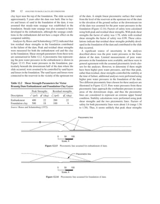


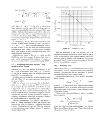


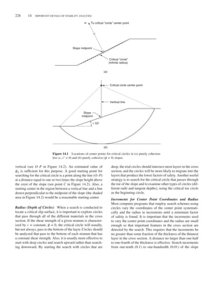


![Duncan c14.tex V2 - 06/20/2014 4:11 P.M. Page˜241
OTHER DETAILS 241
The corresponding shear strength on the slip surface is then
determined from the following:
𝜏ff =
𝜎1 − 𝜎3
2
cos 𝜙′
=
1
2
𝛾z
[
tan2
(
45 +
𝜙′
2
)
− 1
]
(14.9)
where 𝜏ff is the shear stress on the failure plane at failure.
The shear strength, s = 𝜏ff, can be calculated from
Eq. (14.9) and entered into the slope stability calculations as
a cohesion (s = c = 𝜏ff) that increases linearly with depth,
together with 𝜙 = 0. This approach is simple and seems to
work reasonably well. If the zone where the problem occurs
does not have a major impact on the stability of the slope,
Ladd’s simple approach is adequate.
Use the Ordinary Method of Slices Very large or negative
normal stresses at the toe of the slope do not occur in the
Ordinary Method of Slices. The normal force on the base
of the slice varies from a value equal to the weight of the
slice (when the base is horizontal) to zero (when the base of
the slice is vertical). Thus, if problems occur in the passive
zone with other limit equilibrium procedures, the Ordinary
Method of Slices can be used.
Change the Side Force Inclination The final remedy for
eliminating tension near the toe of the slip surface is to
change the inclination of the interslice forces in the area
where the problem occurs. Figure 14.17 can be used to deter-
mine an appropriate interslice force inclination that is con-
sistent with the slip surface inclination in the passive shear
zone. Depending on the developed friction angle (𝜙d) and
slip surface inclination (𝛼), an appropriate interslice force
inclination (𝜃) can be determined from Figure 14.17. The in-
clination can be used directly as the assumed interslice force
inclination in force equilibrium slope stability calculations.
However, this can only be done with force equilibrium pro-
cedures. The interslice force inclination cannot be changed
directly in other limit equilibrium procedures, although the
inclination can be changed indirectly in the Morgenstern
and Price and Chen and Morgenstern procedures through the
assumed values for f(x) and g(x).
Discussion Slope stability calculations in which critical
noncircular slip surfaces have been located show that the
critical slip surface exits the toe of the slope at angles very
similar to what would be expected based on passive earth
pressure theory (i.e., the inclinations agree well with those
shown in Figure 14.17). Thus, it is generally sufficient to
initiate a search with a reasonable starting angle (45 degrees
or less, depending on the shear strength properties of the
soil), and the critical slip surface is then usually found
without problems. It is also helpful to place constraints on
the inclination of the slip surface in an automatic search for
a noncircular slip surface to avoid very steep slip surfaces
being considered at the toe of the slope. Many computer
programs that search for critical noncircular slip surfaces
contain provisions for limiting the steepness of the slip
surfaces where they exit the slope.
Use of the appropriate passive inclination for the slip sur-
face appears to be the most realistic solution to problems
at the toe of the slope and probably conforms most closely
with conditions in the field. The only instances where one
of the other techniques described needs to be employed is
when circular slip surfaces are being used. In these cases the
second and third options—calculation of the strength inde-
pendently, and using the Ordinary Method of Slices—usually
work well.
Recapitulation
• Very large positive or negative forces may develop
on the sides and bottom of slices when the slip sur-
face is steep near the toe of the slope, and the forces
act in directions that are significantly different from
the directions corresponding to minimum passive
earth pressures.
• The problem of inappropriate stresses at the toe of
the slip surface is best remedied by changing the
inclination of the slip surface so that it corresponds
more closely to the inclination of the shear plane for
passive earth pressures.
• The problem of inappropriate stresses at the toe
of a slope may also be remedied by (1) estimat-
ing shear strength directly based on Rankine pas-
sive earth pressure theory, (2) using the Ordinary
Method of Slices, or (3) changing the interslice force
inclination.
14.5 OTHER DETAILS
Additional details that affect the results of slope stability
calculations include the number of slices into which the soil
mass is divided and the tolerances used to define convergence
in the iterative procedures for calculating factors of safety.
14.5.1 Iteration Tolerances and Convergence
All procedures except the infinite slope and the Ordinary
Method of Slices procedures require an iterative (trial-and-
error) process to calculate the factor of safety for a given slip
surface. The iterative process requires one or more conver-
gence criteria to define when a sufficiently accurate solution
for the factor of safety has been found. Convergence crite-
ria can be specified in terms of maximum allowable changes
in the calculated values of factor of safety on successive
iterations, or limits on the magnitude of allowable force and](https://image.slidesharecdn.com/soilstrengthandslopestability-220624112511-a82802bd/85/Soil-Strength-and-Slope-Stability-pdf-257-320.jpg)


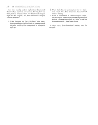


![ANALYSIS SUMMARY FIGURE 251
1
1 2 3 4 5 6 7 8 9 10 11 12 13 14 15 16
2
3
4
5
6
7
8
9
10
20.0
35.2
65.0
62.5
89.9
105.7
21.2
81.8
114.7
49.8
13.1
20.8
10.0
29.5
52.5
82.2
101.4
92.2
54.1
14.2
140
140
140
140
140
140
140
140
140
140
120
120
120
120
120
120
120
120
120
120
36659
215174
683527
894190
1406585
1648280
315386
1055716
867907
98993
43.2
40.2
35.0
28.7
21.7
13.1
7.7
3.4
–4.8
–11.7
25110
138831
391572
429214
519784
374514
42435
62854
–72569
–20099
1891646 3050560
1.613
0
0
0
0
0
0
0
0
0
0
38
20
20
20
20
20
20
38
38
38
0.0
23.2
38.3
55.3
59.9
34.2
11.5
12.9
7.2
0.0
0
1450
2392
3449
3741
2131
719
805
452
0
28641
59724
192187
247055
389600
517970
109240
773349
637567
77342
1.06
0.91
0.95
0.99
1.01
1.03
1.02
1.03
0.96
0.88
27011
65660
202533
250670
384751
505280
106965
752971
666912
87806
0.0
26.6
76.0
84.9
69.1
34.2
5.6
0.0
0.0
0.0
Trial F = 1.613
b cʹ
W u
hshell hcore
γshell γcore
Note: Trial F adjusted repeatedly until computed value, Fʹ, and trial value are the same.
Slice
No.
α W sin α hpiez
Σ
cʹb
+
(W
–ub)
tan
ϕʹ
cʹb
+
(W
–ub)
tan
ϕʹ
Ÿ
m
α
mα
ϕʹ
= Σ =
Fʹ =
Figure 15.1 Sample spreadsheet for Simplified Bishop Procedure.
Table 15.1 Sample Description of Contents of Spreadsheet Presented in Figure 15.1
Column no. Description
1 Slice number
2 Horizontal width of slice
3 Height of portion of slice in the shell material; measured at midpoint of slice, hshell
4 Total unit weight of shell material, 𝛾shell
5 Height of portion of slice in the core material; measured at midpoint of slice, hcore
6 Total unit weight of core material, 𝛾core
7 Weight of slice, W = b(𝛾shellhshell + 𝛾corehcore)
8 Inclination of the bottom of the slice, 𝛼, in degrees measured from the horizontal [positive when the bottom of
the slice is inclined in the same direction as the slope face (e.g., near the crest of the slope); negative when
the base of the slice is inclined in the direction opposite that of the slope face (e.g., near the toe of the slope)]
9 Product of slice weight and sine of the angle, 𝛼
10 Cohesion value for soil at bottom of slice
11 Friction angle for soil at bottom of slice
12 Height of pieizometric line (hpiez) above the center of the base of the slice
13 Pore water pressure at the center of the bottom of the slice, u = 𝛾waterhpiez
14 Intermediate term used to compute numerator in equation for factor of safety: c′b + (W − ub) tan 𝜙′
15 Value of the quantity m𝛼 for trial factor of safety; trial factor of safety is shown above column
15 (m𝛼 = cos 𝛼 + sin 𝛼 tan 𝜙′∕F)
16 Column 14 divided by column 15, representing terms in the numerator of the expression for factor of safety;
column 16 summed for all slices and divided by the summation of column 9 to compute a new factor of
safety, F′](https://image.slidesharecdn.com/soilstrengthandslopestability-220624112511-a82802bd/85/Soil-Strength-and-Slope-Stability-pdf-267-320.jpg)


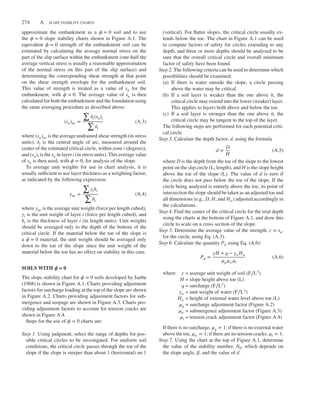


![Duncan bapp01.tex V2 - 06/24/2014 4:03 P.M. Page˜286
286 A SLOPE STABILITY CHARTS
Calculate Pe:
Pe =
𝛾H + q − 𝛾wH′
w
𝜇q𝜇′
w
=
(115)(40) + 0 − (62.4)(30)
(1)(0.96)
= 2870 psf
Estimate cav = 120 psf and 𝜙av = 33 degrees:
𝜆c𝜙 =
Pe tan 𝜙
c
=
(2870)(0.64)
120
= 15.3
From Figure A.5, with b = 1.5 and 𝜆c𝜙 = 15.3:
x0 = 0 and y0 = 1.9
X0 = (H)(x0) = (40)(0) = 0 ft
Y0 = (H)(y0) = (40)(1.9) = 76 ft
Plot the critical circle on the given slope as shown in
Figure A.12. Calculate cav, tan 𝜙av, and 𝜆c𝜙 as follows:
cav =
∑
𝛿ici
∑
𝛿i
=
(19)(100) + (42)(150)
19 + 42
= 134 psf
tan 𝜙av =
∑
𝛿i tan 𝜙i
∑
𝛿i
=
(19)(tan 35∘) + (42)(tan 30∘)
19 + 42
= 0.62
𝜆c𝜙 =
(2870)(0.62)
134
= 13.3
From Figure A.5, with b = 1.5 and 𝜆c𝜙 = 13.3:
x0 = 0.02 and y0 = 1.85
X0 = (H)(x0) = (40)(0.02) = 0.8 ft
Y0 = (H)(y0) = (40)(1.85) = 74 ft
This circle is close to the previous iteration, so keep 𝜆c𝜙 =
13.3 and cav = 134 psf. From Figure A.5, with b = 1.5 and
𝜆c𝜙 = 13.3, Ncf = 35. Calculate the factor of safety:
F = Ncf
c
Pd
= 35
(
134
4141
)
= 1.13
with F = 1.13, the slope would be very close to failure.
Example A.5. Figure A.13 shows a slope where a rela-
tively thin layer of soil overlies firm soil. The critical failure
mechanism for this example is sliding along a plane paral-
lel to the slope, at the top of the firm layer. This slope can
be analyzed using the infinite slope stability chart shown in
Figure A.7. Calculate the factor of safety for seepage paral-
lel to the slope and for horizontal seepage emerging from the
slope.
For seepage parallel to the slope:
X = 8 ft and T = 11.3 ft
ru =
X
T
𝛾w
𝛾
cos2
𝛽 =
8
11.3
(
62.4
120
)
(0.94)2
= 0.325
From Figure A.7, with ru = 0.325 and cot 𝛽 = 2.75, A = 0.62
and B = 3.1. Calculate the factor of safety:
F = A
tan 𝜙′
tan 𝛽
+ B
c′
𝛾H
= 0.62
(
0.577
0.364
)
+ 3.1
[
300
(120) (12)
]
= 0.98 + 0.65 = 1.63
For horizontal seepage emerging from slope, 𝜃 = 0 degree:
ru =
𝛾w
𝛾
1
1 + tan 𝛽 tan 𝜃
=
62.4
120
[
1
1 + (0.364) (0)
]
= 0.52
From Figure A.7, with ru = 0.52 and cot 𝛽 = 2.75, A = 0.41
and B = 3.1. Calculate the factor of safety:
F = A
tan 𝜙′
tan 𝛽
+ B
c′
𝛾H
= 0.41
(
0.577
0.364
)
+ 3.1
[
300
(120) (12)
]
= 0.65 + 0.65 = 1.30
Note that the factor of safety for seepage emerging from the
slope is smaller than the factor of safety for seepage parallel
to the slope.
Example A.6. Figure A.14 shows a submerged clay slope
with 𝜙 = 0 and strength increasing linearly with depth.
Surface of seepage
Seepage parallel to slope
γ = 120 pcf
cʹ = 300 psf
ϕʹ = 30°
tan ϕʹ = 0.577
β = 20°
tan β = 0.364
cot β = 2.75
11.3 ft 8 ft
12 ft
20°
Figure A.13 Infinite slope analysis.](https://image.slidesharecdn.com/soilstrengthandslopestability-220624112511-a82802bd/85/Soil-Strength-and-Slope-Stability-pdf-302-320.jpg)
![Duncan bapp01.tex V2 - 06/24/2014 4:03 P.M. Page˜287
EXAMPLES 287
45°
Submerged
slope
1
0
cu
1
H0 = 15 ft
H = 100 ft
1150 psf
γ = 100 pcf
γb = 37.6 pcf
150 psf
Figure A.14 𝜙 = 0, and strength increasing with depth.
The factor of safety is calculated using the slope stability
chart shown in Figure A.8. Extrapolating the strength profile
up to zero gives H0 = 15 ft. Calculate M as follows:
M =
H0
H
=
15
100
= 0.15
From Figure A.8, with M = 0.15 and 𝛽 = 45 degrees, N =
5.1. From the soil strength profile, cb = 1150 psf. Calculate
the factor of safety:
F = N
cb
𝛾(H + H0)
= 5.1
[
1150
(37.6) (115)
]
= 1.36](https://image.slidesharecdn.com/soilstrengthandslopestability-220624112511-a82802bd/85/Soil-Strength-and-Slope-Stability-pdf-303-320.jpg)


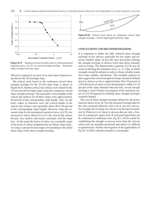


![Duncan b01.tex V3 - 07/16/2014 2:31 P.M. Page˜297
REFERENCES 297
Bromwell, L. G., and Carrier, W. D. I. (1979). Consolidation of
fine-grained mining wastes, Proceedings of 6th Pan-American
Conference on Soil Mechanics and Foundation Engineering,
Vol. 1, Lima, Peru, pp. 293–304.
Bromwell, L. G., and Carrier, W. D. I. (1983). Reclamation alterna-
tives for phosphatic clay disposal areas. Symposium on Surface
Mining, Hydrology, Sedimentology and Reclamation, University
of Kentucky, Lexington, pp. 371–376.
Browzin, B. S. (1961). Non-steady flow in homogeneous earth
dams after rapid drawdown, Proceedings of the Fifth Interna-
tional Conference on Soil Mechanics and Foundation Engineer-
ing, Paris, Vol. 2, pp. 551–554.
Busbridge, J. R., Chan, P., Milligan, V., La Rochelle, P., and
Lefebvre, L. D. (1985). Draft report on “The effect of geogrid
reinforcement on the stability of embankments on a soft sensi-
tive Champlain clay deposit,” Prepared for the Transportation
Development Center, Montreal, Quebec, by Golder Associates
and Laval University.
Byrne, J. (2003). Personal communication.
Byrne, R. J., Kendall, J., and Brown, S. (1992). Cause and mecha-
nism of failure, Kettlemen Hills Landfill B-19, Unit IA, Proceed-
ings ASCE Specialty Conference on Performance and Stability of
Slopes and Embankments—II, Vol. 2, pp. 1188–1215.
Carter, M., and Bentley, S. P. (1985). The geometry of slip surfaces
beneath landslides: Predictions from surface measurements,
Canadian Geotechnical Journal, 22(2), 234–238.
Casagrande, A. (1937). Seepage through dams, Journal of the New
England Water Works Association, 51(2), June [reprinted in Con-
tributions to Soil Mechanics 1925–1940, Boston Society of Civil
Engineers, Boston, 1940, pp. 295–336.]
Celestino, T. B., and Duncan, J. M. (1981). Simplified search for
noncircular slip surfaces, Proceedings of the Tenth International
Conference on Soil Mechanics and Foundation Engineering,
Stockholm, Vol. 3, June, pp. 391–394.
Chandler, R. J. (1977). Back analysis techniques for slope stabiliza-
tion works: A case record, Géotechnique, 27(4), 479–495.
Chandler, R. J. (1988). The in-situ measurement of the undrained
shear strength of clays using the field vane, Vane Shear Strength
Testing in Soils: Field & Lab Studies, STP 1014, ASTM, West
Conshohocken, PA, pp. 13–44.
Chandler, R. J. (1991). Slope stability engineering: Developments
and applications. Proceedings of the International Conference
on Slope Stability, Isle of Wight, England, Thomas Telford,
London.
Chang, C. Y., and Duncan, J. M. (1970). Analysis of soil movements
around a deep excavation, Journal of the Soil Mechanics and
Foundation Division, 96(SM5), 1655–1681.
Charles, J. A., and Soares, M. M. (1984). Stability of compacted
rockfill slopes, Géotechnique, 34(1), 61–70.
Charles, J. A., and Watts, K. S. (1980). The influence of confining
pressure on the shear strength of compacted rockfill, Géotech-
nique, 30(4), 353–397.
Chen, L. T., and Poulos, H. G. (1997). Piles subjected to lateral
soil movements, Journal of Geotechnical and Geoenvironmental
Engineering, 123(9), 802–811.
Chen, Z.-Y., and Morgenstern, N. R. (1983). Extensions to the
generalized method of slices for stability analysis, Canadian
Geotechnical Journal, 20(1), 104–119.
Chen, Z.-Y., and Shao, C. M. (1988). Evaluation of minimum
factor of safety in slope stability analysis, Canadian Geotech-
nical Journal, 25(4), 735–748.
Chirapuntu, S., and Duncan, J. M. (1975). The Role of Fill Strength
in the Stability of Embankments on Soft Clay Foundations,
Geotechnical Engineering Report No. TE 75-3, University of
California, Berkeley.
Chirapuntu, S., and Duncan, J. M. (1977). Cracking and progressive
failure of embankments on soft clay foundations, Proceedings of
the International Symposium on Soft Clay, Bangkok, Thailand,
pp. 453–470.
Chopra, A. K. (1967). Earthquake response of earth dams, Jour-
nal of the Soil Mechanics and Foundations Division, 93(SM2),
65–81.
Christian, J. T. (1996). Reliability methods for stability of existing
slopes, Uncertainty in the Geologic Environment: From Theory
to Practice, Proceedings of Uncertainty ’96, ASCE Geotechnical
special publication No. 58, Madison, WI, pp. 409–418.
Christian, J. T., and Alfredo, U. (1998). Probabilistic evaluation of
earthquake-induced slope failure, Journal of Geotechnical and
Geoenvironmental Engineering, 1140–1143.
Christian, J. T., and Baecher, G. B. (2001). Discussion on “Factors
of safety and reliability in geotechnical engineering by J. M.
Duncan,” Journal of Geotechnical and Geoenvironmental Engi-
neering, 127(8), 700–702.
Christian, J. T., Ladd, C. C., and Baecher, G. B. (1994). Reliabil-
ity applied to slope stability analysis, Journal of Geotechnical
Engineering, 120(12), 2180–2207.
Chugh, A. K. (1981). Pore water pressures in natural slopes, Inter-
national Journal for Numerical Methods in Geomechanics, 5(4),
449–454.
Chugh, A. K. (1982). Procedure for design of restraining structures
for slope stabilization problems, Geotechnical Engineering, 13,
223–234.
Coatsworth, A. M. (1985). A rational approach to consolidated
undrained triaxial testing, Proceedings for the 20th Regional
Meeting, Engineering Group, Guildford, U.K., Geological Soci-
ety, Vol. 1.
Collins, I. F., Gunn, C. I. M., Pender, M. J., and Wang Y. (1988).
Slope stability analysis for materials with a nonlinear failure
envelope, International Journal for Numerical and Analytical
Methods in Geomechanics, 12(5), 533–550.
Collins, S. A., Rogers, W., and Sowers, G. F. (1982). Report of
Embankment Reanalysis—Mohicanville Dikes, Report to the
Huntington District, U.S. Army Corps of Engineers, Hunt-
ington, West Virginia, by Law Engineering Testing Company,
July.
Cooper, M. R. (1984). The application of back-analysis to the
design of remedial works for failed slopes, Proceedings, Fourth
International Symposium on Landslides, Toronto, Vol. 2,
pp. 387–392.
Crabb, G. I., and Atkinson, J. H. (1988). Determination of soil
strength parameters for the analysis of highway slope failures,
Slope Stability Engineering—Developments and Applications,
Proceedings of the International Conference on Slope, Stability,
Institute of Civil Engineers.
Cruden, D. M. (1986). The geometry of slip surfaces beneath
landslides: Predictions from surface measurements: Discussion,
Canadian Geotechnical Journal, 23(1), 94.
Dai, S. H., and Wang, M. O. (1992). Reliability Analysis in Engi-
neering Applications, Van Nostrand Reinhold, New York.
Das, B. M. (2002). Principles of Geotechnical Engineering, 5th ed.,
Brooks/Cole, Pacific Grove, CA.
Decourt, L. (1990). The standard penetration test: state of the art
report, NGI Publication No. 179, Oslo, Norway.
De Mello, V. F. B. (1977). Reflections on design decisions of prac-
tical significance to embankment dams, Géotechnique, 27(3),
281—354.](https://image.slidesharecdn.com/soilstrengthandslopestability-220624112511-a82802bd/85/Soil-Strength-and-Slope-Stability-pdf-313-320.jpg)


