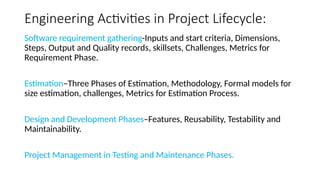
Engineering Activities inProject Lifecycle:
Software requirement gathering-Inputs and start criteria, Dimensions,
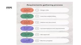
Steps, Output and Quality records, skillsets, Challenges, Metrics for
Requirement Phase.
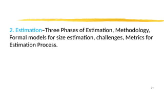
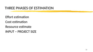
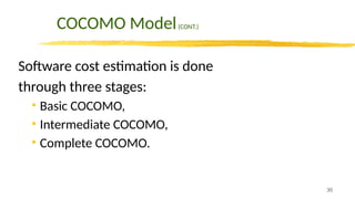
Estimation–Three Phases of Estimation, Methodology, Formal models for
size estimation, challenges, Metrics for Estimation Process.
Design and Development Phases–Features, Reusability, Testability and
Maintainability.
Project Management in Testing and Maintenance Phases.
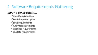
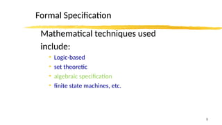
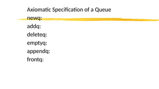
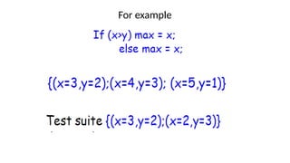
Functional specification usingpre-condition and post
condition
e.g. Module Sort – Sort a list L of integers in ascending
order
Pre-Condt – non-null L
Post-Condt – for all ‘i’, 1<=i<= size {L}, L[i]<=L[i+1]
L=[1,8,7,6,5]
L=[3,4,5,6,8]
10
11.
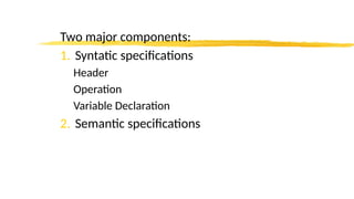
E – InitialState
E’ – Final State
Input : non null L
Output : for all i , 1<=i<size{L’} and L[i]<=l’[i+1] and
L’=permutation[L]
11
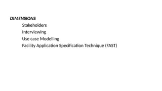
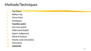
Methods/Techniques
1. Top Down
2.Bottom Up
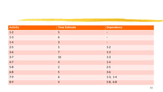
3. Three Point
4. Analogous
5. Function point
6. Use case points
7. Wide band Delphi
8. Expert Judgement
9. What if Analysis
10. Monte Carlo Simulation
11. Parametric
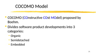
12. COCOMO
24
31
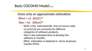
Basic COCOMO Model(CONT.)
Givesonly an approximate estimation:
Effort = a1 (KLOC)a2
Tdev = b1 (Effort)b2
• KLOC is the estimated kilo lines of source code,
• a1,a2,b1,b2 are constants for different
categories of software products,
• Tdev is the estimated time to develop the
software in months,
• Effort estimation is obtained in terms of person
months (PMs).
34
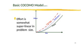
Basic COCOMO Model(CONT.)
Effort is
somewhat
super-linear in
problem size.
Effort
Size
Em
bedded
Sem
idetached
Organic
35.
35
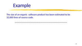
Example
The size ofan organic software product has been estimated to be
32,000 lines of source code.
36.
36
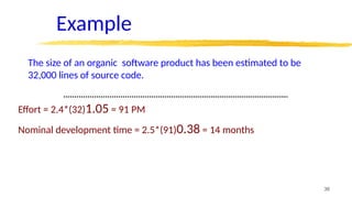
Example
The size ofan organic software product has been estimated to be
32,000 lines of source code.
Effort = 2.4*(32)1.05 = 91 PM
Nominal development time = 2.5*(91)0.38 = 14 months
37.
37
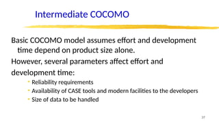
Intermediate COCOMO
Basic COCOMOmodel assumes effort and development
time depend on product size alone.
However, several parameters affect effort and
development time:
• Reliability requirements
• Availability of CASE tools and modern facilities to the developers
• Size of data to be handled
39
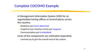
Complete COCOMO Example
AManagement Information System (MIS) for an
organization having offices at several places across
the country:
• Database part (semi-detached)
• Graphical User Interface (GUI) part (organic)
• Communication part (embedded)
Costs of the components are estimated separately:
• summed up to give the overall cost of the system.
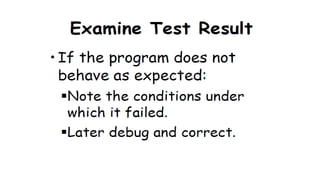
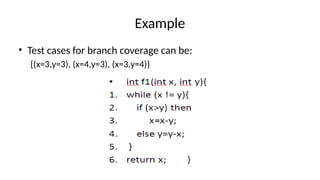
Example
• Test casesfor branch coverage can be:
{(x=3,y=3), (x=4,y=3), (x=3,y=4)}
59.
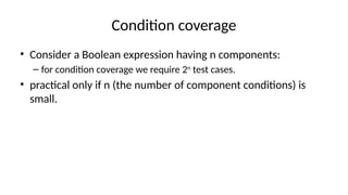
Condition coverage
• Considera Boolean expression having n components:
– for condition coverage we require 2n
test cases.
• practical only if n (the number of component conditions) is
small.
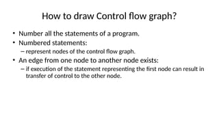
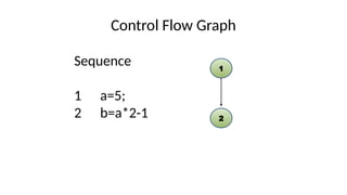
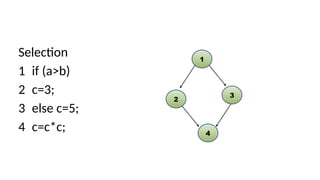
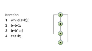
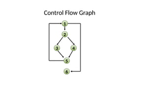
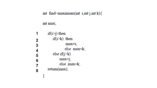
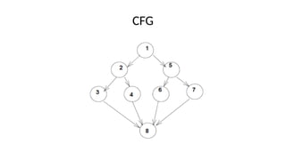
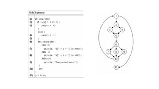
How to drawControl flow graph?
• Number all the statements of a program.
• Numbered statements:
– represent nodes of the control flow graph.
• An edge from one node to another node exists:
– if execution of the statement representing the first node can result in
transfer of control to the other node.
Cyclomatic complexity
• Anotherway of computing cyclomatic complexity:
– determine number of bounded areas in the graph
• Any region enclosed by a nodes and edge sequence.
• V(G) = Total number of bounded areas + 1
65.
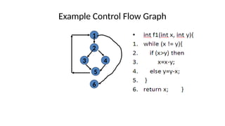
Example
• From avisual examination of the CFG:
– the number of bounded areas is 2.
– cyclomatic complexity = 2+1=3.
66.
Cyclomatic complexity
• McCabe'smetric provides:
– a quantitative measure of estimating testing difficulty
– Amenable to automation
• Intuitively,
– number of bounded areas increases with the number of decision
nodes and loops.
67.
Cyclomatic complexity
• Thecyclomatic complexity of a program provides:
– a lower bound on the number of test cases to be designed
– to guarantee coverage of all linearly independent paths.
68.
Cyclomatic complexity
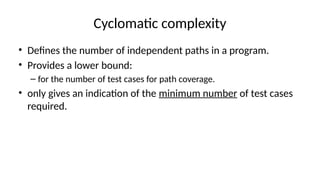
• Definesthe number of independent paths in a program.
• Provides a lower bound:
– for the number of test cases for path coverage.
• only gives an indication of the minimum number of test cases
required.
69.
Path testing
• Thetester proposes initial set of test data using his experience
and judgement.
70.
An interesting applicationof cyclomatic complexity
• Relationship exists between:
– McCabe's metric
– the number of errors existing in the code,
– the time required to find and correct the errors.
71.
Cyclomatic complexity
• Cyclomaticcomplexity of a program:
– also indicates the psychological complexity of a program.
– difficulty level of understanding the program.
72.
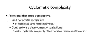
Cyclomatic complexity
• Frommaintenance perspective,
– limit cyclomatic complexity
• of modules to some reasonable value.
– Good software development organizations:
• restrict cyclomatic complexity of functions to a maximum of ten or so.
73.
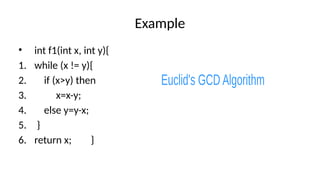
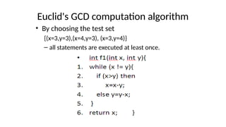
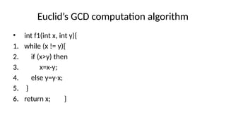
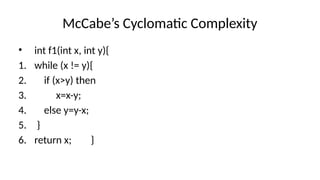
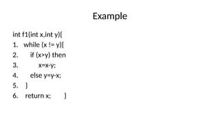
Euclid’s GCD computationalgorithm
• int f1(int x, int y){
1. while (x != y){
2. if (x>y) then
3. x=x-y;
4. else y=y-x;
5. }
6. return x; }
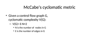
McCabe's cyclomatic metric
•Given a control flow graph G,
cyclomatic complexity V(G):
– V(G)= E-N+2
• N is the number of nodes in G
• E is the number of edges in G
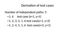
Derivation of testcases
Number of independent paths: 3
–1, 6 test case (x=1, y=1)
–1, 2, 3, 5, 1, 6 test case(x=1, y=2)
–1, 2, 4, 5, 1, 6 test case(x=2, y=1)
Data Flow-Based Testing
•For a statement numbered S,
– DEF(S) = {X/statement S contains a definition of X}
– USES(S)= {X/statement S contains a use of X}
– Example: 1: a=b; DEF(1)={a}, USES(1)={b}.
– Example: 2: a=a+b; DEF(1)={a}, USES(1)={a,b}.
91.
Project SizeEstimation Techniques - Software Engineeri
ng
– GeeksforGeeks
6 Success
What is an Estimation Method? 6 Project Planning Tips
[2024] • Asana
ful Project Estimation Techniques in 2024
92

![Functional specification using pre-condition and post
condition
e.g. Module Sort – Sort a list L of integers in ascending
order
Pre-Condt – non-null L
Post-Condt – for all ‘i’, 1<=i<= size {L}, L[i]<=L[i+1]
L=[1,8,7,6,5]
L=[3,4,5,6,8]
10](https://image.slidesharecdn.com/module4-250312042814-8c54e6cc/85/Software-engineering-module-4-notes-for-btech-and-mca-10-320.jpg)
![E – Initial State
E’ – Final State
Input : non null L
Output : for all i , 1<=i<size{L’} and L[i]<=l’[i+1] and
L’=permutation[L]
11](https://image.slidesharecdn.com/module4-250312042814-8c54e6cc/85/Software-engineering-module-4-notes-for-btech-and-mca-11-320.jpg)

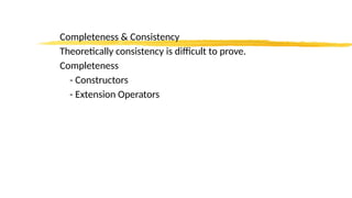
![1. Stack [integer] Header
Declare
2. Create() Stack; Constructors
3. Push(stack, integer) Stack;
4. Pop(stack) stack;
5. Top(stack) integer or undefined; Extension Operators
Var
6. s: stack ; i: integer ; Variable declaration
For all
7. top(create())=undefined;
8. top(push(s,i))=I;
9. pop(create())=create(); Axioms
10. pop(push(s,i))=s;
end](https://image.slidesharecdn.com/module4-250312042814-8c54e6cc/85/Software-engineering-module-4-notes-for-btech-and-mca-16-320.jpg)
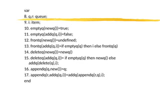
![1. queue[item] header
declare
2. newq() queue;
3. addq(queue, item) queue;
4. deleteq(queue) queue;
5. emptyq(queue) Boolean;
6. appendq(queue,queue) queue;
7. frontq(queue) Item or undefined;](https://image.slidesharecdn.com/module4-250312042814-8c54e6cc/85/Software-engineering-module-4-notes-for-btech-and-mca-18-320.jpg)
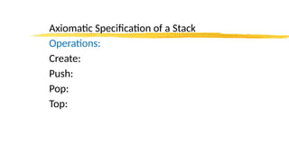
![FP=UFP*[0.65+0.01*46]
FP=50*1.11=55.5 => 56
1 FP=60 LOC
56 * 60 =3360 LOC
FP - Domain Count Weighting Factor Value
EI 3 3 9
EO 2 4 8
EQ 2 3 6
ILF 1 7 7
EIF 4 5 20
28](https://image.slidesharecdn.com/module4-250312042814-8c54e6cc/85/Software-engineering-module-4-notes-for-btech-and-mca-28-320.jpg)


![ Project Size Estimation Techniques - Software Engineeri
ng
– GeeksforGeeks
6 Success
What is an Estimation Method? 6 Project Planning Tips
[2024] • Asana
ful Project Estimation Techniques in 2024
92](https://image.slidesharecdn.com/module4-250312042814-8c54e6cc/85/Software-engineering-module-4-notes-for-btech-and-mca-91-320.jpg)