Waarom timeseries
Wat zijntimeseries
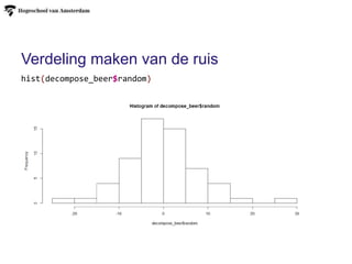
Decompositie van timeseries
Basis functies voor timeseries
Stabiliseren van timeseries
Omgaan met NA in timeseries
Analyse van de ruis (AR/MA/white noise)
4.
CREDITS TO
• MichelangeloVargas voor vak 3.4 SEC
• NA n dataset http://publish.illinois.edu/spencer-guerrero/2014/12/11/2-dealing-
with-missing-data-in-r-omit-approx-or-spline-part-1/
• Decompositie https://anomaly.io/seasonal-trend-decomposition-in-r/
• Basis functies https://cran.r-project.org/doc/contrib/Ricci-refcard-ts.pdf
• AR/MA modelleren https://www.analyticsvidhya.com/blog/2015/12/complete-
tutorial-time-series-modeling/
• Forecast https://media.readthedocs.org/pdf/a-little-book-of-r-for-time-
series/latest/a-little-book-of-r-for-time-series.pdf
5.
Het doel vandit college is
• Data kunt ombouwen naar timeseries
• Tijdreeks formules begrijpen
• Tijdreeksen transformeren middels decompositie
• Met de timeseries package kunt werken
6.
Waarom timeseries
Een voorbeeld
Eris een distributie-centrum met producten die in opslag zijn en
producten die niet in opslag zijn. Dit heeft te maken met het aantal
bestellingen per maand. Verschillende mensen in het bedrijf
vermoeden dat het aantal bestellingen van een bepaald product stijgt.
Hoe controleren we dit? Wat zullen de bestellingen in de
toekomst zijn?
7.
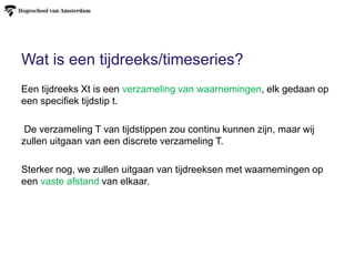
Wat is eentijdreeks/timeseries?
Een tijdreeks Xt is een verzameling van waarnemingen, elk gedaan op
een specifiek tijdstip t.
De verzameling T van tijdstippen zou continu kunnen zijn, maar wij
zullen uitgaan van een discrete verzameling T.
Sterker nog, we zullen uitgaan van tijdreeksen met waarnemingen op
een vaste afstand van elkaar.
8.
Een tijdreeks ismeestal een samenstelling
van componenten
Voor het beschrijven van een tijdreeks maken we gebruik van vier
componenten.
• De trend De trend geeft de globale beschrijving van de stijging of
daling van een tijdreeks.
• De seizoencomponent Deze component geeft het cyclische
gedrag van de tijdreeks. De periode van dit gedrag hoort constant
en bekend te zijn.
• De conjunctuurcomponent Deze component geeft het cyclische
gedrag waarvan de periode niet bekend is. Deze periode zal over
het algemeen langer zijn dan de seizoensperiode.
• De toevallige component Dit is het gedrag dat we niet kunnen
beschrijven met de drie andere componenten.
9.
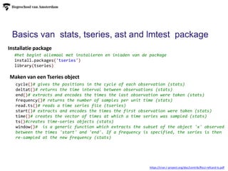
Basics van stats,tseries, ast and lmtest package
cycle()# gives the positions in the cycle of each observation (stats)
deltat()# returns the time interval between observations (stats)
end()# extracts and encodes the times the last observation were taken (stats)
frequency()# returns the number of samples per unit time (stats)
read.ts()# reads a time series file (tseries)
start()# extracts and encodes the times the first observation were taken (stats)
time()# creates the vector of times at which a time series was sampled (stats)
ts()#creates time-series objects (stats)
window()# is a generic function which extracts the subset of the object 'x' observed
between the times 'start' and 'end'. If a frequency is specified, the series is then
re-sampled at the new frequency (stats)
#het begint allemaal met installeren en inladen van de package
install.packages('tseries')
library(tseries)
Maken van een Tseries object
Installatie package
https://cran.r-project.org/doc/contrib/Ricci-refcard-ts.pdf
10.
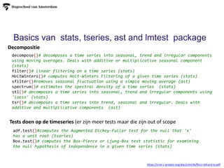
Tests doen opde timeseries (er zijn meer tests maar die zijn out of scope
Decompositie
https://cran.r-project.org/doc/contrib/Ricci-refcard-ts.pdf
decompose()# decomposes a time series into seasonal, trend and irregular components
using moving averages. Deals with additive or multiplicative seasonal component
(stats)
filter()# linear filtering on a time series (stats)
HoltWinters()# computes Holt-Winters Filtering of a given time series (stats)
sfilter()#removes seasonal fluctuation using a simple moving average (ast)
spectrum()# estimates the spectral density of a time series (stats)
stl()# decomposes a time series into seasonal, trend and irregular components using
'loess' (stats)
tsr()# decomposes a time series into trend, seasonal and irregular. Deals with
additive and multiplicative components (ast)
adf.test()#computes the Augmented Dickey-Fuller test for the null that 'x'
has a unit root (tseries)
Box.test()# computes the Box-Pierce or Ljung-Box test statistic for examining
the null hypothesis of independence in a given time series (stats)
Basics van stats, tseries, ast and lmtest package
11.
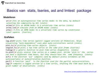
Grafieken
Modelleren
https://cran.r-project.org/doc/contrib/Ricci-refcard-ts.pdf
Basics van stats,tseries, ast and lmtest package
ar()# fits an autoregressive time series model to the data, by default
selecting the complexity by AIC (stats)
arima()# fits an ARIMA model to a univariate time series (stats)
arima.sim()# simulate from an ARIMA model (stats)
arma() # fits an ARMA model to a univariate time series by conditional
least squares (tseries)
lag.plot# plots time series against lagged versions of themselves. Helps
visualizing "auto-dependence" even when auto-correlations vanish (stats)
plot.ts()# plotting time-series objects (stats)
seqplot.ts()# plots a two time series on the same plot frame (tseries)
tsdiag()# a generic function to plot time-series diagnostics (stats)
ts.plot()# plots several time series on a common plot. Unlike 'plot.ts' the series
can have a different time bases, but they should have the same frequency (stats)
acf() # the function 'acf' computes (and by default plots) estimates of the
autocovariance or autocorrelation function.
pacf() # Function 'pacf' is the function used for the partial autocorrelations.
lag()# computes a lagged version of a time series, shifting the time base back by a
given number of observations (stats)
12.
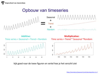
Opbouw van timeseries
Additive:
Timeseries = Seasonal + Trend + Random
https://anomaly.io/seasonal-trend-decomposition-in-r/
Multiplicative:
Time series = Trend * Seasonal *Random
kijk goed naar de twee figuren en vertel hoe je het verschil ziet
13.
https://drsifu.wordpress.com/2012/11/27/time-series-econometrics/
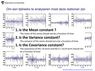
1.Is the Meanconstant ?
The mean of the series should not be a function of time
2.Is the Variance constant?
The variance of the series should not a be a function of time.
1.Is the Covariance constant?
The covariance of the i th term and the (i + m) th term should not
be a function of time
Om een tijdreeks te analyseren moet deze stationair zijn
14.
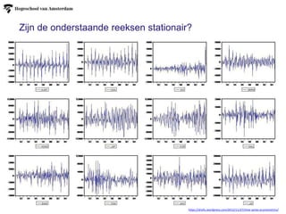
Zijn de onderstaandereeksen stationair?
https://drsifu.wordpress.com/2012/11/27/time-series-econometrics/
15.
https://www.analyticsvidhya.com/blog/2015/12/complete-tutorial-time-series-modeling/
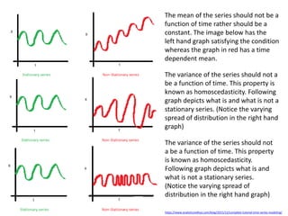
The mean ofthe series should not be a
function of time rather should be a
constant. The image below has the
left hand graph satisfying the condition
whereas the graph in red has a time
dependent mean.
The variance of the series should not a
be a function of time. This property is
known as homoscedasticity. Following
graph depicts what is and what is not a
stationary series. (Notice the varying
spread of distribution in the right hand
graph)
The variance of the series should not
a be a function of time. This property
is known as homoscedasticity.
Following graph depicts what is and
what is not a stationary series.
(Notice the varying spread of
distribution in the right hand graph)
16.
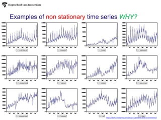
Examples of nonstationary time series WHY?
https://drsifu.wordpress.com/2012/11/27/time-series-econometrics/
17.
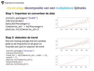
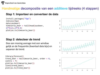
Handmatige decompositie vaneen additieve tijdreeks (4 stappen)
Stap 1: Importeer en converteer de data
Stap 2: detecteer de trend
install.packages("fpp")
library(fpp)
data(ausbeer)
timeserie_beer = tail(head(ausbeer,
17*4+2),17*4-4)
plot(as.ts(timeserie_beer))
Doe een moving average met een window
gelijk an de frequentie (kwartaal data bijv) en
separeer de trend.
library(forecast)
trend_beer = ma(timeserie_beer, order = 4,
centre = T)
plot(as.ts(timeserie_beer))
lines(trend_beer)
plot(as.ts(trend_beer))
18.
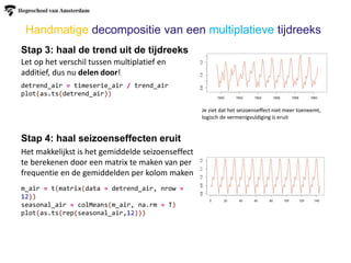
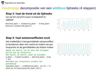
Handmatige decompositie vaneen additieve tijdreeks (4 stappen)
Stap 3: haal de trend uit de tijdreeks
Stap 4: haal seizoenseffecten eruit
Het makkelijkst is het gemiddelde seizoenseffect
te berekenen door een matrix te maken van per
frequentie en de gemiddelden per kolom maken
detrend_beer = timeserie_beer - trend_beer
plot(as.ts(detrend_beer))
Let op het verschil tussen multiplatief en
additief
#maak een matrix van de data met kolommen
gelijk aan de frequentie
#en kantel de matrix zodat de kolommen
m_beer = t(matrix(data = detrend_beer, nrow
= 4))
#bereken per frequentie element het
gemiddelde
seasonal_beer = colMeans(m_beer, na.rm = T)
plot(as.ts(rep(seasonal_beer,16)))
19.
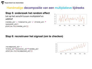
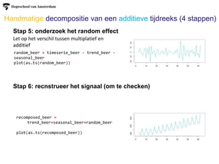
Handmatige decompositie vaneen additieve tijdreeks (4 stappen)
Stap 5: onderzoek het random effect
Stap 6: recnstrueer het signaal (om te checken)
Let op het verschil tussen multiplatief en
additief
random_beer = timeserie_beer - trend_beer -
seasonal_beer
plot(as.ts(random_beer))
recomposed_beer =
trend_beer+seasonal_beer+random_beer
plot(as.ts(recomposed_beer))
20.
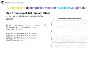
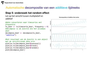
Automatische decompositie vaneen additieve tijdreeks
Stap 5: onderzoek het random effect
Let op het verschil tussen multiplatief en
additief
#data converteren naar timeseries met
frequentie
ts_beer <- ts(timeserie_beer, frequency = 4)
#decompose is de functie die het allemaal
doet
decompose_beer <- decompose(ts_beer,
"additive")
#het resultaat van de functie is een object
met de verschillende data erin
plot(as.ts(decompose_beer$seasonal))
plot(as.ts(decompose_beer$trend))
plot(as.ts(decompose_beer$random))
plot(decompose_beer)
21.
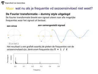
Maar wat nuals je frequentie vd sezoensinvloed niet weet?
De Fourier transformatie – dummy style uitgelegd
De Fourier transformatie breekt een signaal uiteen naar alle mogelijke
frequenties waar het signaal uit bestaat:
een sinus een samengesteld signaal
Het resultaat is een grafiek waarbij de pieken de frequenties van de
seizoensinvloed zijn, denk erom frequentie dus T = 1 / f
Sin(ϖt)
22.
Maar wat nuals je frequentie vd sezoensinvloed niet weet?
De Fourier transformatie in R
https://anomaly.io/detect-seasonality-using-fourier-transform-r/
# Install and import TSA package
install.packages("TSA")
library(TSA)
# Lees een dataset in
raw = read.csv("iets.csv")
# compute the Fourier Transform
p = periodogram(vectormetwaarden)
#let op dit is een object met data erin!
#maak df met frequenie en spec = hoogte piek
dd = data.frame(freq=p$freq, spec=p$spec)
#rangschik df van hoge naar lage pieken
order = dd[order(-dd$spec),]
#pak de belangijkste 2 (of meer) pieken eruit
top2 = head(order, 2)
# display the 2 highest "power" frequencies
top2
# convert frequency to time periods
time = 1/top2$f
time
23.
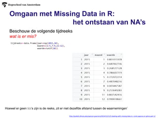
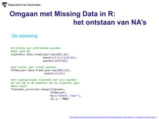
Omgaan met MissingData in R:
het ontstaan van NA’s
Beschouw de volgende tijdreeks
wat is er mis?
http://publish.illinois.edu/spencer-guerrero/2014/12/11/2-dealing-with-missing-data-in-r-omit-approx-or-spline-part-1/
tijdreeks<-data.frame(jaar=rep(2015,10),
maand=c(1:5,7:9,11:12),
waarde=runif(10))
Hoewel er geen NA’s zijn is de reeks, zit er niet dezelfde afstand tussen de waarnemingen`
24.
Omgaan met MissingData in R:
het ontstaan van NA’s
Beschouw de volgende tijdreeks
wat is er mis?
http://publish.illinois.edu/spencer-guerrero/2014/12/11/2-dealing-with-missing-data-in-r-omit-approx-or-spline-part-1/
tijdreeks<-data.frame(jaar=rep(2015,10),
maand=c(1:5,7:9,11:12),
waarde=runif(10))
Hoewel er geen NA’s zijn is de reeks, zit er niet dezelfde afstand tussen de waarnemingen`
1
2
3
4
5
7
8
9
11
12
1
2
3
4
5
6
7
8
9
10
11
12
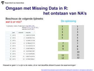
De oplossing
25.
Omgaan met MissingData in R:
het ontstaan van NA’s
http://publish.illinois.edu/spencer-guerrero/2014/12/11/2-dealing-with-missing-data-in-r-omit-approx-or-spline-part-1/
De oplossing
#tijdreeks met ontbrekende maanden
#maar geen NA
tijdreeks<-data.frame(jaar=rep(2015,10),
maand=c(1:5,7:9,11:12),
waarde=runif(10))
#een totaal jaar zonder waarden
TOTAALjaar<-data.frame(jaar=rep(2015,12),
maand=c(1:12))
#een samengevoegde tijdreeks met alle maanden
#en met NA op de momenten dat de tijdreeks geen
#data heeft
Tijdreeks_correctie<-merge(tijdreeks,
TOTAALjaar,
by=c("maand","jaar"),
all.y = TRUE)
26.
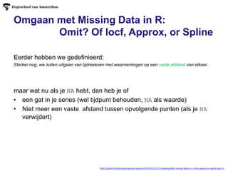
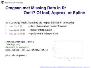
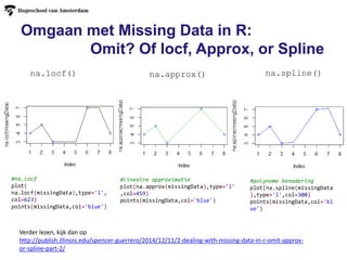
Omgaan met MissingData in R:
Omit? Of locf, Approx, or Spline
Eerder hebben we gedefinieerd:
Sterker nog, we zullen uitgaan van tijdreeksen met waarnemingen op een vaste afstand van elkaar.
maar wat nu als je NA hebt, dan heb je of
• een gat in je series (wel tijdpunt behouden, NA als waarde)
• Niet meer een vaste afstand tussen opvolgende punten (als je NA
verwijdert)
http://publish.illinois.edu/spencer-guerrero/2014/12/11/2-dealing-with-missing-data-in-r-omit-approx-or-spline-part-1/
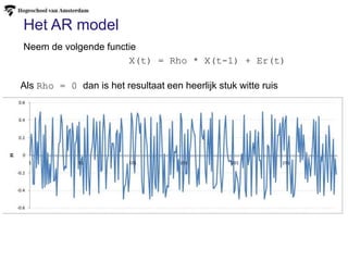
Het AR model
X(t)= Rho * X(t-1) + Er(t)
Neem de volgende functie
Als Rho = 0 dan is het resultaat een heerlijk stuk witte ruis
32.
Het AR model
X(t)= Rho * X(t-1) + Er(t)
Neem de volgende functie
Als Rho = 0.5 wat voor verschil zie je dan?
33.
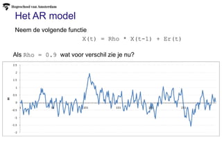
Het AR model
X(t)= Rho * X(t-1) + Er(t)
Neem de volgende functie
Als Rho = 0.9 wat voor verschil zie je nu?
34.
Het AR model
X(t)= Rho * X(t-1) + Er(t)
Neem de volgende functie
Als Rho = 1.0 dan hebben we een random walk
Die niet stationair is want E[X(t)] = Rho *E[ X(t-1)]
35.
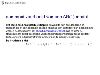
een mooi voorbeeldvan een AR(1) model
Het bruto nationaal product (bnp) is de waarde van alle goederen en
diensten die in een bepaalde periode (meestal een jaar) door een bepaald land
worden geproduceerd: het bruto binnenlands product plus de door de
staatsburgers in het buitenland verdiende primaire inkomens minus de door
buitenlanders in het betreffende land verdiende primaire inkomens.
De hypthese is dat
BNP(t) = alpha * BNP(t – 1) + error (t)
36.
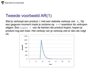
Tweede voorbeeld AR(1)
Stelje verkoopt een product X met een stabiele verkoop van X0. Op
een gegeven moment maak je reclame op t=9 waardoor de verkopen
stijgen. Een alpha % van de klanten die product kopen, kopen je
product nog een keer. Het verloop van je verkoop ziet er dan als volgt
uit.
37.
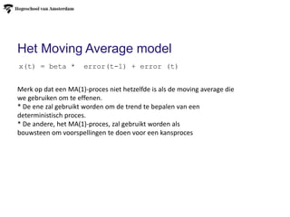
Het Moving Averagemodel
x(t) = beta * error(t-1) + error (t)
Merk op dat een MA(1)-proces niet hetzelfde is als de moving average die
we gebruiken om te effenen.
* De ene zal gebruikt worden om de trend te bepalen van een
deterministisch proces.
* De andere, het MA(1)-proces, zal gebruikt worden als
bouwsteen om voorspellingen te doen voor een kansproces
38.
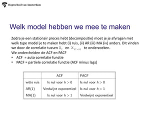
Welk model hebbenwe mee te maken
Zodra je een stationair proces hebt (decompositie) moet je je afvragen met
welk type model je te maken hebt (i) ruis, (ii) AR (iii) MA (iv) anders. Dit vinden
we door de correlatie tussen Xt en X(t-n) te onderzoeken.
We ondercheiden de ACF en PACF
• ACF = auto correlatie functie
• PACF = partiele correlatie functie (ACF minus lags)
39.
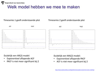
Welk model hebbenwe mee te maken
Timeseries 1 geeft onderstaande plot Timeseries 2 geeft onderstaande plot
Duidelijk een AR(2) model:
• Exponentieel aflopende ACF
• PACF is niet meer significant bij 2
https://www.analyticsvidhya.com/blog/2015/12/complete-tutorial-time-series-modeling/
Duidelijk een MA(2) model:
• Exponentieel aflopende PACF
• ACF is niet meer significant bij 2
40.
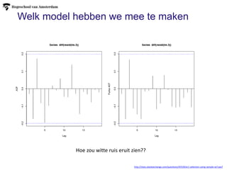
Welk model hebbenwe mee te maken
http://stats.stackexchange.com/questions/45539/ar1-selection-using-sample-acf-pacf
Hoe zou witte ruis eruit zien??
41.
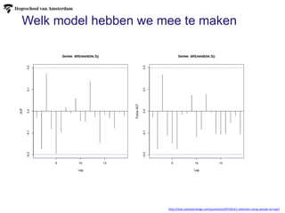
Welk model hebbenwe mee te maken
http://stats.stackexchange.com/questions/45539/ar1-selection-using-sample-acf-pacf
42.
Forecasts using ExponentialSmoothing
Exponential smoothing can be used to make short-term forecasts for
time series data.
http://a-little-book-of-r-for-time-
series.readthedocs.io/en/latest/src/timeseries.html
43.
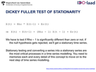
DICKEY FULLER TESTOF STATIONARITY
X(t) = Rho * X(t-1) + Er(t)
X(t) - X(t-1) = (Rho - 1) X(t - 1) + Er(t)
We have to test if Rho – 1 is significantly different than zero or not. If
the null hypothesis gets rejected, we’ll get a stationary time series.
Stationary testing and converting a series into a stationary series are
the most critical processes in a time series modelling. You need to
memorize each and every detail of this concept to move on to the
next step of time series modelling.
https://www.analyticsvidhya.com/blog/2015/12/complete-tutorial-time-series-modeling/
44.
Handmatige decompositie vaneen multiplatieve tijdreeks
Stap 1: Importeer en converteer de data
Stap 2: detecteer de trend
Doe een moving average met een window
gelijk an de frequentie (in dit geval 12
maanden per jaar) en separeer de trend.
install.packages("Ecdat")
library(Ecdat)
data(AirPassengers)
timeserie_air = AirPassengers
plot(as.ts(timeserie_air))
install.packages("forecast")
library(forecast)
trend_air = ma(timeserie_air, order = 12,
centre = T)
plot(as.ts(timeserie_air))
lines(trend_air)
plot(as.ts(trend_air))
45.
Stap 3: haalde trend uit de tijdreeks
Stap 4: haal seizoenseffecten eruit
Het makkelijkst is het gemiddelde seizoenseffect
te berekenen door een matrix te maken van per
frequentie en de gemiddelden per kolom maken
Let op het verschil tussen multiplatief en
additief, dus nu delen door!
Handmatige decompositie van een multiplatieve tijdreeks
detrend_air = timeserie_air / trend_air
plot(as.ts(detrend_air))
Je ziet dat het seizoenseffect niet meer toeneemt,
logisch de vermenigvuldiging is eruit
m_air = t(matrix(data = detrend_air, nrow =
12))
seasonal_air = colMeans(m_air, na.rm = T)
plot(as.ts(rep(seasonal_air,12)))
46.
Stap 5: onderzoekhet random effect
Stap 6: recnstrueer het signaal (om te checken)
Let op het verschil tussen multiplatief en
additief
random_air = timeserie_air / (trend_air *
seasonal_air)
plot(as.ts(random_air))
recomposed_air =
trend_air*seasonal_air*random_air
plot(as.ts(recomposed_air))
Handmatige decompositie van een multiplatieve tijdreeks
47.
Stap 5: onderzoekhet random effect
Let op het verschil tussen multiplatief en
additief
Automatische decompositie van een multiplatieve tijdreeks
ts_air = ts(timeserie_air, frequency = 12)
decompose_air = decompose(ts_air,
"multiplicative")
plot(as.ts(decompose_air$seasonal))
plot(as.ts(decompose_air$trend))
plot(as.ts(decompose_air$random))
plot(decompose_air)
Editor's Notes
#9 http://www.emathzone.com/tutorials/basic-statistics/components-of-time-series.html
The factors that are responsible to bring about changes in a time series, also called the components of time series, are as follows:
Secular Trend (or General Trend)
Seasonal Movements
Cyclical Movements
Irregular Fluctuations
Secular Trend:
The secular trend is the main component of a time series which results from long term effect of socio-economic and political factors. This trend may show the growth or decline in a time series over a long period. This is the type of tendency which continues to persist for a very long period. Prices, export and imports data, for example, reflect obviously increasing tendencies over time.
Seasonal Trend:
These are short term movements occurring in a data due to seasonal factors. The short term is generally considered as a period in which changes occur in a time series with variations in weather or festivities. For example, it is commonly observed that the consumption of ice-cream during summer us generally high and hence sales of an ice-cream dealer would be higher in some months of the year while relatively lower during winter months. Employment, output, export etc. are subjected to change due to variation in weather. Similarly sales of garments, umbrella, greeting cards and fire-work are subjected to large variation during festivals like Valentine’s Day, Eid, Christmas, New Year etc. These types of variation in a time series are isolated only when the series is provided biannually, quarterly or monthly.
Cyclic Movements:
These are long term oscillation occurring in a time series. These oscillations are mostly observed in economics data and the periods of such oscillations are generally extended from five to twelve years or more. These oscillations are associated to the well known business cycles. These cyclic movements can be studied provided a long series of measurements, free from irregular fluctuations is available.
Irregular Fluctuations:
These are sudden changes occurring in a time series which are unlikely to be repeated, it is that component of a time series which cannot be explained by trend, seasonal or cyclic movements .It is because of this fact these variations some-times called residual or random component. These variations though accidental in nature, can cause a continual change in the trend, seasonal and cyclical oscillations during the forthcoming period. Floods, fires, earthquakes, revolutions, epidemics and strikes etc,. are the root cause of such irregularities.


![Maar wat nu als je frequentie vd sezoensinvloed niet weet?
De Fourier transformatie in R
https://anomaly.io/detect-seasonality-using-fourier-transform-r/
# Install and import TSA package
install.packages("TSA")
library(TSA)
# Lees een dataset in
raw = read.csv("iets.csv")
# compute the Fourier Transform
p = periodogram(vectormetwaarden)
#let op dit is een object met data erin!
#maak df met frequenie en spec = hoogte piek
dd = data.frame(freq=p$freq, spec=p$spec)
#rangschik df van hoge naar lage pieken
order = dd[order(-dd$spec),]
#pak de belangijkste 2 (of meer) pieken eruit
top2 = head(order, 2)
# display the 2 highest "power" frequencies
top2
# convert frequency to time periods
time = 1/top2$f
time](https://image.slidesharecdn.com/b45a867f-7e43-43c0-b5f7-bef222e5a5c5-161024134345/85/Software-Engineering-College-6-timeseries-data-22-320.jpg)

![Het AR model
X(t) = Rho * X(t-1) + Er(t)
Neem de volgende functie
Als Rho = 1.0 dan hebben we een random walk
Die niet stationair is want E[X(t)] = Rho *E[ X(t-1)]](https://image.slidesharecdn.com/b45a867f-7e43-43c0-b5f7-bef222e5a5c5-161024134345/85/Software-Engineering-College-6-timeseries-data-34-320.jpg)