Social

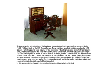
1. This equipment is representative of the tabulating system invented and developed by Herman Hollerith
(1860-1929) and built for the U.S. Census Bureau. These machines were first used in compiling the 1890
Census. Hollerith's patents were acquired by the Computing-Tabulating-Recording Co. (which later became
IBM), and this work became the basis of the IBM Punched Card System. The first "tabulator" used simple
clock-like counting devices. When an electrical circuit is closed (through a punched hole in a predetermined
position on the card), each counter is actuated by an electromagnet. The unit's pointer (clock hand) moves
one step each time the magnet is energized. The circuits to the electromagnets are closed by means of a
hand-operated press type card reader. The operator places each card in the reader, pulls down a lever, and
removes the card after each punched hole is counted.
- IBM Archives (http://www-03.ibm.com/ibm/history/exhibits/attic/attic_071.html)

2. 2
COMP 206:
Computer Architecture and
Implementation
Montek Singh
Jan 27-29, 2009
Lecture 4: Instruction Set Architecture

3. Approaching an ISA
 Instruction Set Architecture
 Defines set of operations, instruction format, hardware
supported data types, named storage, addressing modes,
sequencing
 Meaning of each instruction is described by RTL on
architected registers and memory
3

4. 4
Moving Toward Design
 Given technology constraints assemble adequate datapath
 Architected storage mapped to actual storage
 Function units to do all the required operations
 Possible additional storage (eg. MAR)
 Interconnect to move information among regs and FUs
 Map each instruction to sequence of RTLs
 Collate sequences into symbolic controller state transition
diagram (STD)
 Implement controller

5. Datapath vs Control
 Datapath: Storage, FU, interconnect sufficient to perform the desired
functions
 Inputs are Control Points
 Outputs are signals (such as overflow, negative, etc)
 Controller: State machine to orchestrate operation on the data path
 Based on desired function and signals
5
Datapath Controller
Control Points
signals

6. 6
Contents
 Design objectives
 Information representation
 Endian-ness, aligned access
 Organization of Instructions
 Encoding

7. 7
Instruction Set Design Objective #1
Code size (code density):
 Depends on:
size of MM/cache
access time of cache (on-chip/off-chip)
CPU-MM bandwidth
 Frequently used instructions should be short
 Implies variable-length instructions
But there are negatives to this

8. Instruction Set Design Objective #2
Execution speed (performance) :
 Only frequently executed instructions should be included in the instruction set
 Infrequently executed instructions slow down the others
 Complex and long instructions tend to be used infrequently
 Defining hardware-software interface
 Frequently executed instructions should be fast
 Pipelining should be made as easy as possible
 Overlapped execution lowers CPI value
 Single instruction length, simple instruction formats, and few addressing
modes for easy decoding
 Three (register) address instructions decouple CPU and memory
8

9. 9
Instruction Set Design Objective #3
Minimize size and complexity of hardware
(ALU/Control)
 Implementing infrequently executed instructions ties down
hardware that is rarely used, and could be used for some
other purpose with greater advantage

10. Instruction Set Design Objective #4
Instruction set as a programming language
 Needs of a human programmer (less important today)
 Several desirable properties of instruction sets have been recognized and described,
such as orthogonality (each operand can be specified independently of the others)
and consistency (being able to predict the remainder of an architecture given partial
knowledge of the system)
 Needs of an optimizing compiler
 Simple instructions are more suitable for code optimizations
 Optimizing compilers try to find the shortest or fastest code sequence that
implements the semantics of a HLL program. To make code reorganization
tractable, an instruction set is needed that makes:
– the size of each instruction easy to calculate;
– the execution time of each instruction easy to calculate;
– the interactions between instructions easy to figure out.
 ISA features such as complex addressing modes, variable length instructions,
special-purpose registers provide too many ways of doing the same thing and lead
to combinatorial explosion
10

11. Notations for Information Representation
11
64 bits
8 bytes
2 words
1 doubleword
Q: How do we number these various units of information in a consistent manner?
9 6 2 1 7 6 6
Most Significant Digit (MSD)
“Big End”
Least Significant Digit (LSD)
“Little End”
0 1 2 3 4 5 6
“Big End”-ian Numbering
6 5 4 3 2 1 0 “Little End”-ian Numbering
“On holy wars and a plea for peace”, Danny Cohen, IEEE Computer 14(10), pages 49-54, Oct 1981

12. Why Is Numbering Important?
 English text is written left-to-right and the characters are numbered left-
to-right
 Numbers can be numbered in two different ways
 Memory locations are numbered (addresses)
 Consequences of numbering
 Data is stored in memory according to byte numbering (the lower-numbered byte goes
into a byte in memory with a smaller address)
 Data is sent through a bit-serial communication channel according to bit numbering (bit 0
goes first, followed by bit 1, etc.)
 When displaying computer representation for humans
 Numbers are written in the usual way (MSD on left, LSD on right)
 Text is written in such a way as to match the numbering of numbers
12

13. Odds and Ends about Numbering
 The Little Endian notation is compatible with mathematical
conventions of positional notation
 The Little Endian notation has the disadvantage that is
displays English text in reverse
 To overcome this, manuals for Little Endian machines usually display character
strings vertically
 Example machines
 Little Endian: PDP-11, VAX, 80x86
 Big Endian: IBM 370, MIPS, DLX, SPARC
 Mixed: Motorola 68000, Z8000
 Big Endian byte ordering
 Little Endian bit ordering
13

14. Alignment of Words in Memory
 CPU accesses a 32-bit word of data starting at byte address x…x00
 Such an address (multiple of 32[b]/8[b/B] = 4[B]) is called word-aligned
 Memory controller is simple and fast, data available in one cycle
 CPU accesses a 32-bit word of data starting at byte address 01111
 Byte addresses are 01111, 10000, 10001, 10010 (misaligned address)
 Doubles the access time of word
 Requiring aligned addresses results in simpler memory controller and faster
execution
 Costs some loss of storage, and adds complexity in code generators
14
32 bits
Mem
Bank
00
8
Mem
Bank
01
8
Mem
Bank
10
8
Mem
Bank
11
8
Memory
Controller

15. Sub-Word Accesses
 Byte operand in register is usually the rightmost byte of register
 Byte may come from any of the four memory banks
 Needs routing/permuting hardware
 Either at memory side of bus (justified bus)
Byte always travels on rightmost quarter of bus
 Or on CPU side (unjustified bus)
Bus lanes are extensions of memory bank lanes
 Source of complications in either case 15
32 bits
Mem
Bank
00
8
Mem
Bank
01
8
Mem
Bank
10
8
Mem
Bank
11
8
Memory
Controller
CPU
Register
File
(32 bits)

16. What is Used?
16
SPEC2000

17. Organization of an Instruction
Uniform Variable
Length
Opcode
Number Where How specified
Operands Specifiers
Format
Syntax
Processing Data movement Transfer of control I/O operations
Semantics
Machine instruction
Arithmetic
Logical
Shift
(e.g., MIPS:
4 bytes)
(e.g., VAX:
1-37 bytes)
0 address
1 address
2 address
3 address
implied
Instruction
Register
Memory
Addressing modes
•immediate
•absolute
•computed
Load (from MM)
Store (to MM)
Move (reg-reg)
Move (MM-MM)
Unconditional (branch)
Conditional (jump)
Call
Return
If I/O is not
memory-
mapped
1) Length of operands
2) Shift/rotate: direction,
amount
3) Branch condition

18. Operand Locations
18

19. Classification by Operands
Stack Accumulator General Purpose Register
Load/Store Reg/Mem Mem/Mem
ALU operations 0 address 1 address 3 address 2 (or 1.5) address 3 address
Explicit operands (1,1) (0,3) (1,2), (1, 3), (2, 2) (3, 3)
Instruction size Short Short 4 bytes 2/4/6 bytes variable
Needs separate Load/Store Load/Store Load/Store Store
Early examples Burroughs PDP-8 CDC 6600 IBM S/360 DEC VAX-11/780
B5000- Intel 8086 IBM S/370
B7500 Motorola 6809
Current examples Transputer All RISC machines IBM 3033, IBM S/390
Amdahl V
Hitachi, Fujitsu
Orthogonality Farthest from Intermediate Closest to
Pipelining Easiest Intermediate Hardest
19
 Important machines that are difficult to classify
 Intel 80x86
 variable instruction size: 1-17 bytes
 memory can be destination
 uses implied registers
 Motorola 680x0
 Instruction size: 2, 4, 6, 8, 10 bytes
 Two address format only (2, 2)
(m,n) means
m memory operands
n total operands

20. Registers versus Cache
 Similarities
 Both small, fast, and expensive (flip-flops)
 Both used to increase execution speed of CPU
 Both operate based on locality of reference
 Differences
 Registers are visible in ISA; caches are not (except for instructions for invalidation,
prefetch, or flushing)
 Number of registers is fixed by instruction format; size of cache is easily changeable
 Registers have higher BW: 3 words/cycle, and are random-access; caches have lower
BW: 1 word/cycle, and are associative
 Register access time is fixed; cache access time is statistical
 Register allocation is explicit by compiler; cache allocation is automatic
 Registers require fewer bits to address; caches require full memory addresses
 Registers create no I/O problems; caches do
20

21. Organization of Registers
 One general-purpose set (all interchangeable, “typeless”)
 One general-purpose set (a few with dedicated uses)
 PDP-11: eight 16-bit registers (R6: stack pointer, R7: PC)
 VAX 11/780: sixteen 32-bit registers (four special-purpose, R14: stack pointer, R15: PC)
 Two sets
 Motorola 68000: eight 32-bit data, eight 32-bit address
 IBM 370: sixteen 32-bit integer, four 64-bit FP
 DLX, MIPS: 31 32-bit integer, 32 32-bit FP
 Three sets
 CDC 6600: eight 18-bit integer, eight 18-bit address, eight 60-bit FP
 Many registers with dedicated use
 Intel 80x86
21

22. Addressing Modes
 We can’t directly refer to data values, only their addresses
 Except for immediate operands
 Register deferred and direct addressing modes can be synthesized from
displacement addressing mode
22
Name Example Meaning When used
Register add r4, r3 R[r4] := R[r4]+R[r3] When value is in register
Immediate add r4, #3 R[r4] := R[r4]+3 For constants
Displacement add r4, 100(r1) R[r4] := R[r4]+M[100+R[r1]] Accessing local variables
Register deferred add r4, (r1) R[r4] := R[r4] + M[R[r1]] Pointer, computed address
Indexed add r3, (r1+r2) R[r3] := R[r3]+M[R[r1]+R[r2]] Array addressing
Direct add r1, (1001) R[r1] := R[r1]+M[1001] Static data
Memory indirect add r1, @(r3) R[r1] := R[r1]+M[M[R[r3]]] Pointer dereferencing
Autoincrement add r1, (r2)+ R[r1] := R[r1]+M[R[r2]]; R[r2] := R[r2]+d Stepping through array
Autodecrement add r1, -(r2) R[r2] := R[r2]-d; R[r1] := R[r1]+M[R[r2]] Stepping through array
Scaled add r1, 100(r2)[r3] R[r1] := R[r1]+M[100+R[r2]+d*R[r3]] Array indexing
R : the register file
M: the memory address space
d : the size of the data item being accessed (1, 2, 4, 8 bytes)

23. Frequency of Addressing Modes
23
SPEC2000
Register account for ½. This is the other ½.

24. 24
Address Displacement Sizes
This type of data would help you decide how much space to
allocate to displacement. Tested on a machine w/ 16 bits of
displacement, so can’t evaluate more.
SPEC2000

25. Use of Immediate Operands
25

26. 26
Length of Immediate Oper.
Max size was 16. HP book says that a study on
VAX (32-bit imm.) showed 20-25% were longer
than 16 bits

27. 27
Control Transfer Instructions
Terminology
 BTA (Branch Target Address): The destination address of the branch
 The BTA is static if it is always the same during execution
 The BTA is dynamic if it can vary during a single execution of a program (procedure
return, O-O dynamic dispatch, switch statements are major examples)
 Branch taken if next instruction to be executed is at address BTA
 Branch not taken if next instruction to be executed is the one following the branch
instruction (“fall-through”)
 Branch outcome: whether the branch is taken or not taken
 Forward branch: BTA > (PC), where (PC) is the address of the branch instruction
 Backward branch: BTA < (PC)
 An unconditional branch is always taken

28. Code Generation Examples for Branches
28
if (x > 0) y += z;
else y -=z;
blez r7, L18
addu r3, r3, r4
j L33
L18:
subu r3, r3, r4
L33:
while (a < b) {
a++; b--; x++;
}
j L33
L34:
addu r5, r5, 1
addu r6, r6, -1
addu r7, r7, 1
L33:
slt r2, r5, r6
bne r2, r0, L34
Register r3 contains y
Register r4 contains z
Register r5 contains a
Register r6 contains b
Register r7 contains x

29. 29
Classification of Branches
HP terminology Branch Jump Call Return
Conditional Unconditional Unconditional Unconditional
HLL equivalent IF-THEN GOTO CALL RETURN
Relative freq. 83% 5% 6% 6%
Taken With probability T always always always
Not taken With probability 1-T never never never
BTA static most often (PC-relative) PC-relative most frequent never
BTA dynamic usually not allowed BTA in register BTA in register always
Taken Not Taken
F&T F&NT Forward
B&T B&NT Backward
Classifying branches into these four
groups permits us to compute some of the
dynamic frequencies if some others have
been measured.
Rule of thumb: Backward branches tend to be taken,
forward branches tend not to be taken. Why?

30. Evaluating Branch Conditions
30
Name How is condition tested? Advantages Disadvantages
Condition code Special bits set by ALU ops Sometimes condition is Extra state, additional constraints
set for free on instruction reordering
Condition register Test arbitrary register Simple Uses up a register
with result of comparison
Compare and branch Compare is part of branch One instruction rather May be too much work
than two per instruction
 Typical set of condition codes (e.g., Motorola 680x0)
 NegativeResult, ZeroResult, ArithmeticOverflow, CarryOut
 Many RISC machines do not use condition codes (e.g.,
MIPS, Alpha)
 Magnitude comparisons are done with explicit COMPARE instructions
that put their results into named registers
 Some instructions have two variants: one traps on overflow, the
other does not

31. Branch Distance
31

32. 32
Instruction Encoding
These days encoding more important for embedded
processors. PowerPC compresses code in memory,
uncompresses in icache.

33. “Typical” RISC ISA
 32-bit fixed format instruction (3 formats)
 32 32-bit GPR (R0 contains zero, DP take pair)
 3-address, reg-reg arithmetic instruction
 Single address mode for load/store:
base + displacement
 no indirection
 Simple branch conditions
 Delayed branch
33
see: SPARC, MIPS, HP PA-Risc, DEC Alpha, IBM PowerPC,
CDC 6600, CDC 7600, Cray-1, Cray-2, Cray-3

34. Example: MIPS
34
Op
31 26 0
15
16
20
21
25
Rs1 Rd immediate
Op
31 26 0
25
Op
31 26 0
15
16
20
21
25
Rs1 Rs2
target
Rd Opx
Register-Register
5
6
10
11
Register-Immediate
Op
31 26 0
15
16
20
21
25
Rs1 Rs2/Opx immediate
Branch
Jump / Call

35. 35
Next Time
 Pipelining
 If you’ve never looked at pipelining, read Appendix A,
otherwise skim