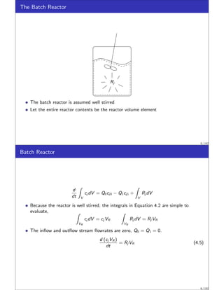
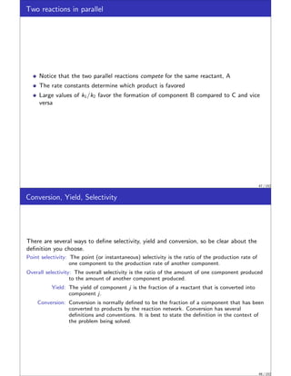
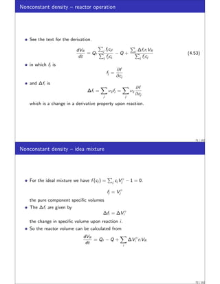
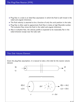
This document discusses material balances for chemical reactors. It begins by introducing the general mole balance equation that applies a conservation of mass principle to chemical components in a reactor system. It then provides analytical solutions to the mole balance equation for some common reaction rate expressions including first-order reversible and irreversible reactions, second-order reactions, and reactions with general nth-order kinetics. It also discusses solutions for series reactions and reactions exhibiting inhibition. The document aims to develop fundamental equations for modeling different reactor systems based on reaction kinetics and component material balances.
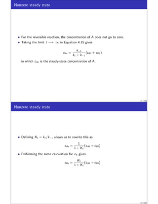
![nth-order, irreversible
A
k
−→ B r = kcn
A
dcA
dt
= −r = −kcn
A
This equation also is separable and can be rearranged to
dcA
cn
A
= −kdt
Performing the integration and solving for cA gives
cA =
h
c−n+1
A0 + (n − 1)kt
i 1
−n+1
, n ̸= 1
31 / 152
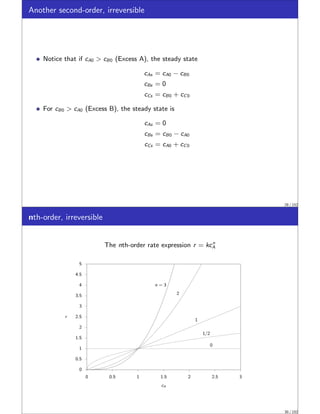
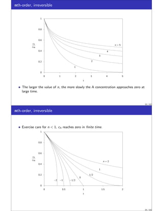
nth-order, irreversible
We can divide both sides by cA0 to obtain
cA
cA0
= [1 + (n − 1)k0t]
1
−n+1 , n ̸= 1 (4.25)
in which
k0 = kcn−1
A0
has units of inverse time.
32 / 152](https://image.slidesharecdn.com/slides-matbal-2up-221102073514-690290f6/85/slides-matbal-2up-pdf-16-320.jpg)
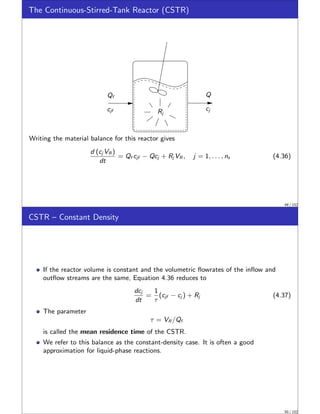
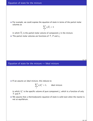
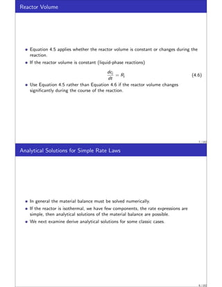
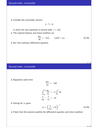
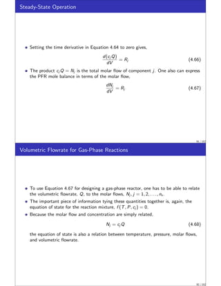
![Thin Disk Volume Element
Expressing the material balance for the volume element
∂ (cj ∆V )
∂t
= cj Q|z − cj Q|z+∆z + Rj ∆V
Dividing the above equation by ∆V and taking the limit as ∆V goes to zero yields,
∂cj
∂t
|{z}
accumulation
= −
∂ (cj Q)
∂V
| {z }
convection
+ Rj
|{z}
reaction
(4.64)
89 / 152
Length or volume as independent variable
If the tube has constant cross section, Ac , then velocity, v, is related to volumetric
flowrate by v = Q/Ac , and axial length is related to tube volume by z = V /Ac ,
Equation 4.64 can be rearranged to the familiar form [1, p.584]
∂cj
∂t
= −
∂ (cj v)
∂z
+ Rj (4.65)
90 / 152](https://image.slidesharecdn.com/slides-matbal-2up-221102073514-690290f6/85/slides-matbal-2up-pdf-45-320.jpg)
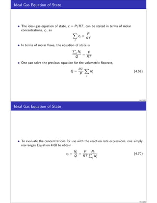
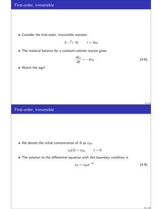
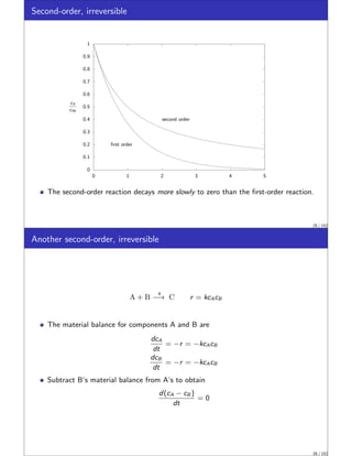
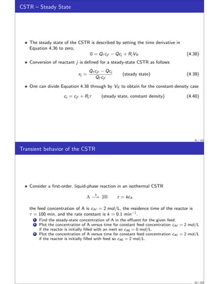
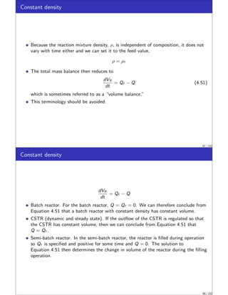
![Changing flowrate in a PFR
Performing the integration gives,
2NAf ln (NA/NAf ) + (NAf − NA) = −
kP
RT
V
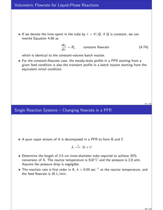
The conversion of component j for a plug-flow reactor operating at steady state is
defined as
xj =
Njf − Nj
Njf
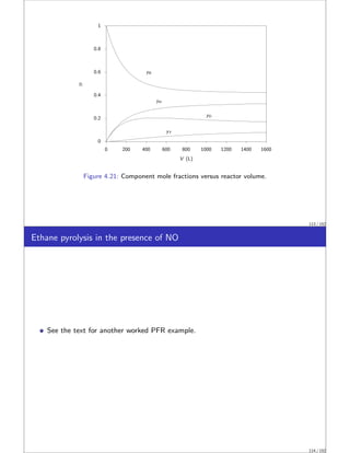
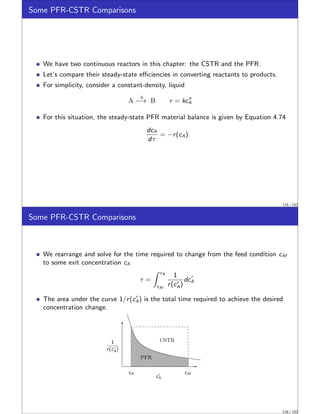
Because we are interested in the V corresponding to 35% conversion of A, we
substitute NA = (1 − xA)NAf into the previous equation and solve for V,
V = −
RT
kP
NAf [2 ln(1 − xA) + xA]
103 / 152
Changing flowrate in a PFR
Because Qf = NAf RT/P is given in the problem statement and the tube length is
desired, it is convenient to rearrange the previous equation to obtain
z = −
Qf
kAc
[2 ln(1 − xA) + xA]
Substituting in the known values gives
z = −
35 × 103
cm3
/min
0.05 sec−1 60 sec/min
4
π(2.5 cm)2
[2 ln(1 − .35) + .35]
z = 1216 cm = 12.2 m
104 / 152](https://image.slidesharecdn.com/slides-matbal-2up-221102073514-690290f6/85/slides-matbal-2up-pdf-52-320.jpg)
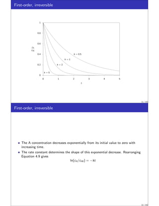
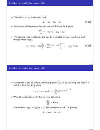
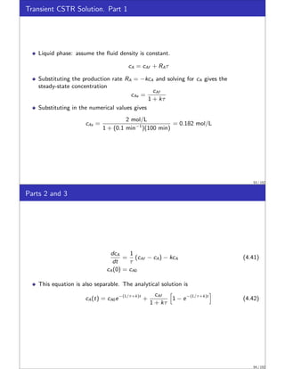
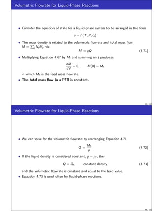
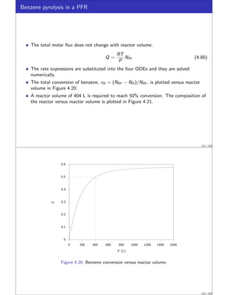
![Multiple-Reaction Systems
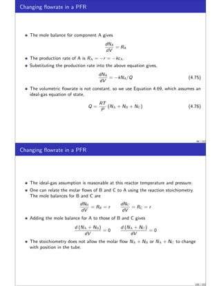
The modeler has some freedom in setting up the material balances for a plug-flow
reactor with several reactions.
The most straightforward method is to write the material balance relation for every
component,
dNj
dV
= Rj , j = 1, 2, . . . , ns
Rj =
nr
X
i=1
νij ri , j = 1, 2, . . . , ns
The reaction rates are expressed in terms of the species concentrations.
The cj are calculated from the molar flows with Equation 4.68
Q is calculated from Equation 4.69, if an ideal-gas mixture is assumed.
105 / 152
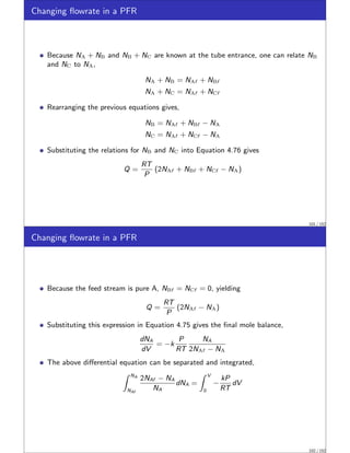
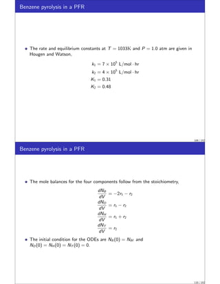
Benzene pyrolysis in a PFR I
Hougen and Watson [3] analyzed the rate data for the pyrolysis of benzene by the
following two reactions.
Diphenyl is produced by the dehydrogenation of benzene,
2C6H6
k1
−⇀
↽−
k−1
C12H10 + H2
2B −⇀
↽− D + H
106 / 152](https://image.slidesharecdn.com/slides-matbal-2up-221102073514-690290f6/85/slides-matbal-2up-pdf-53-320.jpg)
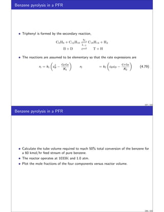
![CSTR Equivalence Principle.
This example was motivated by a recent result of Feinberg and Ellison called the
CSTR Equivalence Principle of Reactor-Separator Systems [2].
This surprising principle states:
For a given reaction network with ni linearly independent reactions, any steady
state that is achievable by any reactor-separator design with total reactor volume
V is achievable by a design with not more than ni + 1 CSTRs, also of total
reactor volume V . Moreover the concentrations, temperatures and pressures in
the CSTRs are arbitrarily close to those occurring in the reactors of the original
design.
123 / 152
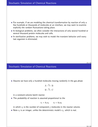
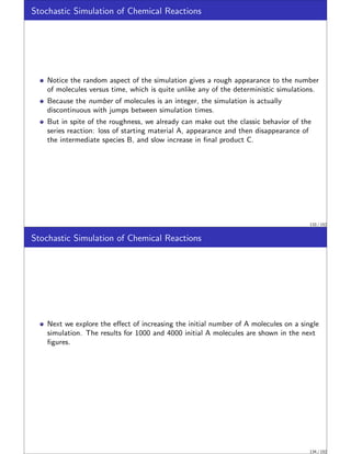
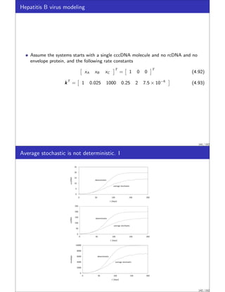
Stochastic Simulation of Chemical Reactions
We wish to introduce next a topic of increasing importance to chemical engineers,
stochastic (random) simulation.
In stochastic models we simulate quite directly the random nature of the molecules.
We will see that the deterministic rate laws and material balances presented in the
previous sections can be captured in the stochastic approach by allowing the
numbers of molecules in the simulation to become large.
The stochastic modeling approach is appropriate if the random nature of the system
is one of the important features to be captured in the model.
These situations are becoming increasingly important to chemical engineers as we
explore reactions at smaller and smaller length scales.
124 / 152](https://image.slidesharecdn.com/slides-matbal-2up-221102073514-690290f6/85/slides-matbal-2up-pdf-62-320.jpg)