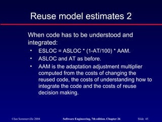
©Ian Sommerville 2004 Software Engineering, 7th edition. Chapter 26 Slide 1
Software cost estimation
©Ian Sommerville 2004 Software Engineering, 7th edition. Chapter 26 Slide 2
Objectives
To introduce the fundamentals of software
costing and pricing
To describe three metrics for software
productivity assessment
To explain why different techniques should
be used for software estimation
To describe the principles of the COCOMO 2
algorithmic cost estimation model
©Ian Sommerville 2004 Software Engineering, 7th edition. Chapter 26 Slide 3
Topics covered
Software productivity
Estimation techniques
Algorithmic cost modelling
Project duration and staffing
©Ian Sommerville 2004 Software Engineering, 7th edition. Chapter 26 Slide 4
Fundamental estimation questions
How much effort is required to complete an
activity?
How much calendar time is needed to
complete an activity?
What is the total cost of an activity?
Project estimation and scheduling are
interleaved management activities.
©Ian Sommerville 2004 Software Engineering, 7th edition. Chapter 26 Slide 5
Software cost components
Hardware and software costs.
Travel and training costs.
Effort costs (the dominant factor in most
projects)
• The salaries of engineers involved in the project;
• Social and insurance costs.
Effort costs must take overheads into account
• Costs of building, heating, lighting.
• Costs of networking and communications.
• Costs of shared facilities (e.g library, staff restaurant,
etc.).
©Ian Sommerville 2004 Software Engineering, 7th edition. Chapter 26 Slide 6
Costing and pricing
Estimates are made to discover the cost, to
the developer, of producing a software
system.
There is not a simple relationship between
the development cost and the price charged
to the customer.
Broader organisational, economic, political
and business considerations influence the
price charged.
©Ian Sommerville 2004 Software Engineering, 7th edition. Chapter 26 Slide 7
Software pricing factors
©Ian Sommerville 2004 Software Engineering, 7th edition. Chapter 26 Slide 8
A measure of the rate at which individual
engineers involved in software development
produce software and associated
documentation.
Not quality-oriented although quality
assurance is a factor in productivity
assessment.
Essentially, we want to measure useful
functionality produced per time unit.
Software productivity
©Ian Sommerville 2004 Software Engineering, 7th edition. Chapter 26 Slide 9
Size related measures based on some
output from the software process. This may
be lines of delivered source code, object
code instructions, etc.
Function-related measures based on an
estimate of the functionality of the delivered
software. Function-points are the best known
of this type of measure.
Productivity measures
©Ian Sommerville 2004 Software Engineering, 7th edition. Chapter 26 Slide 10
Estimating the size of the measure (e.g. how
many function points).
Estimating the total number of programmer
months that have elapsed.
Estimating contractor productivity (e.g.
documentation team) and incorporating this
estimate in overall estimate.
Measurement problems
©Ian Sommerville 2004 Software Engineering, 7th edition. Chapter 26 Slide 11
What's a line of code?
• The measure was first proposed when programs were
typed on cards with one line per card;
• How does this correspond to statements as in Java which
can span several lines or where there can be several
statements on one line.
What programs should be counted as part of the
system?
This model assumes that there is a linear
relationship between system size and volume of
documentation.
Lines of code
©Ian Sommerville 2004 Software Engineering, 7th edition. Chapter 26 Slide 12
The lower level the language, the more
productive the programmer
• The same functionality takes more code to implement in a
lower-level language than in a high-level language.
The more verbose the programmer, the higher
the productivity
• Measures of productivity based on lines of code suggest
that programmers who write verbose code are more
productive than programmers who write compact code.
Productivity comparisons
©Ian Sommerville 2004 Software Engineering, 7th edition. Chapter 26 Slide 13
System development times
©Ian Sommerville 2004 Software Engineering, 7th edition. Chapter 26 Slide 14
Function points
Based on a combination of program characteristics
• external inputs and outputs;
• user interactions;
• external interfaces;
• files used by the system.
A weight is associated with each of these and the
function point count is computed by multiplying each
raw count by the weight and summing all values.
©Ian Sommerville 2004 Software Engineering, 7th edition. Chapter 26 Slide 15
Function points
The function point count is modified by complexity of
the project
FPs can be used to estimate LOC depending on the
average number of LOC per FP for a given language
• LOC = AVC * number of function points;
• AVC is a language-dependent factor varying from 200-
300 for assemble language to 2-40 for a 4GL;
FPs are very subjective. They depend on the
estimator
• Automatic function-point counting is impossible.
©Ian Sommerville 2004 Software Engineering, 7th edition. Chapter 26 Slide 16
Object points
Object points (alternatively named application
points) are an alternative function-related measure
to function points when 4Gls or similar languages
are used for development.
Object points are NOT the same as object classes.
The number of object points in a program is a
weighted estimate of
• The number of separate screens that are displayed;
• The number of reports that are produced by the system;
• The number of program modules that must be developed
to supplement the database code;
©Ian Sommerville 2004 Software Engineering, 7th edition. Chapter 26 Slide 17
Object point estimation
Object points are easier to estimate from a
specification than function points as they are
simply concerned with screens, reports and
programming language modules.
They can therefore be estimated at a fairly
early point in the development process.
At this stage, it is very difficult to estimate
the number of lines of code in a system.
©Ian Sommerville 2004 Software Engineering, 7th edition. Chapter 26 Slide 18
Real-time embedded systems, 40-160
LOC/P-month.
Systems programs , 150-400 LOC/P-month.
Commercial applications, 200-900
LOC/P-month.
In object points, productivity has been
measured between 4 and 50 object
points/month depending on tool support and
developer capability.
Productivity estimates
©Ian Sommerville 2004 Software Engineering, 7th edition. Chapter 26 Slide 19
Factors affecting productivity
©Ian Sommerville 2004 Software Engineering, 7th edition. Chapter 26 Slide 20
All metrics based on volume/unit time are
flawed because they do not take quality into
account.
Productivity may generally be increased at the
cost of quality.
It is not clear how productivity/quality metrics
are related.
If requirements are constantly changing then an
approach based on counting lines of code is not
meaningful as the program itself is not static;
Quality and productivity
©Ian Sommerville 2004 Software Engineering, 7th edition. Chapter 26 Slide 21
Estimation techniques
There is no simple way to make an accurate
estimate of the effort required to develop a software
system
• Initial estimates are based on inadequate information in a
user requirements definition;
• The software may run on unfamiliar computers or use
new technology;
• The people in the project may be unknown.
Project cost estimates may be self-fulfilling
• The estimate defines the budget and the product is
adjusted to meet the budget.
©Ian Sommerville 2004 Software Engineering, 7th edition. Chapter 26 Slide 22
Changing technologies
Changing technologies may mean that previous
estimating experience does not carry over to new
systems
• Distributed object systems rather than mainframe
systems;
• Use of web services;
• Use of ERP or database-centred systems;
• Use of off-the-shelf software;
• Development for and with reuse;
• Development using scripting languages;
• The use of CASE tools and program generators.
©Ian Sommerville 2004 Software Engineering, 7th edition. Chapter 26 Slide 23
Estimation techniques
Algorithmic cost modelling.
Expert judgement.
Estimation by analogy.
Parkinson's Law.
Pricing to win.
©Ian Sommerville 2004 Software Engineering, 7th edition. Chapter 26 Slide 24
Estimation techniques
©Ian Sommerville 2004 Software Engineering, 7th edition. Chapter 26 Slide 25
Pricing to win
The project costs whatever the customer has
to spend on it.
Advantages:
• You get the contract.
Disadvantages:
• The probability that the customer gets the
system he or she wants is small. Costs do not
accurately reflect the work required.
©Ian Sommerville 2004 Software Engineering, 7th edition. Chapter 26 Slide 26
Top-down and bottom-up estimation
Any of these approaches may be used top-
down or bottom-up.
Top-down
• Start at the system level and assess the overall
system functionality and how this is delivered
through sub-systems.
Bottom-up
• Start at the component level and estimate the
effort required for each component. Add these
efforts to reach a final estimate.
©Ian Sommerville 2004 Software Engineering, 7th edition. Chapter 26 Slide 27
Top-down estimation
Usable without knowledge of the system
architecture and the components that might
be part of the system.
Takes into account costs such as integration,
configuration management and
documentation.
Can underestimate the cost of solving
difficult low-level technical problems.
©Ian Sommerville 2004 Software Engineering, 7th edition. Chapter 26 Slide 28
Bottom-up estimation
Usable when the architecture of the system
is known and components identified.
This can be an accurate method if the
system has been designed in detail.
It may underestimate the costs of system
level activities such as integration and
documentation.
©Ian Sommerville 2004 Software Engineering, 7th edition. Chapter 26 Slide 29
Estimation methods
Each method has strengths and weaknesses.
Estimation should be based on several methods.
If these do not return approximately the same result,
then you have insufficient information available to
make an estimate.
Some action should be taken to find out more in
order to make more accurate estimates.
Pricing to win is sometimes the only applicable
method.
©Ian Sommerville 2004 Software Engineering, 7th edition. Chapter 26 Slide 30
Pricing to win
This approach may seem unethical and un-
businesslike.
However, when detailed information is lacking it may
be the only appropriate strategy.
The project cost is agreed on the basis of an outline
proposal and the development is constrained by that
cost.
A detailed specification may be negotiated or an
evolutionary approach used for system
development.
©Ian Sommerville 2004 Software Engineering, 7th edition. Chapter 26 Slide 31
Algorithmic cost modelling
Cost is estimated as a mathematical function of
product, project and process attributes whose
values are estimated by project managers:
• Effort = A × SizeB
× M
• A is an organisation-dependent constant, B reflects the
disproportionate effort for large projects and M is a
multiplier reflecting product, process and people
attributes.
The most commonly used product attribute for cost
estimation is code size.
Most models are similar but they use different values
for A, B and M.
©Ian Sommerville 2004 Software Engineering, 7th edition. Chapter 26 Slide 32
Estimation accuracy
The size of a software system can only be
known accurately when it is finished.
Several factors influence the final size
• Use of COTS and components;
• Programming language;
• Distribution of system.
As the development process progresses
then the size estimate becomes more
accurate.
©Ian Sommerville 2004 Software Engineering, 7th edition. Chapter 26 Slide 33
Estimate uncertainty
x2x4x
0.5x0.25x
FeasibilRequiDesiCodD
©Ian Sommerville 2004 Software Engineering, 7th edition. Chapter 26 Slide 34
The COCOMO model
An empirical model based on project experience.
Well-documented, ‘independent’ model which is not
tied to a specific software vendor.
Long history from initial version published in 1981
(COCOMO-81) through various instantiations to
COCOMO 2.
COCOMO 2 takes into account different approaches
to software development, reuse, etc.
©Ian Sommerville 2004 Software Engineering, 7th edition. Chapter 26 Slide 35
COCOMO 81
©Ian Sommerville 2004 Software Engineering, 7th edition. Chapter 26 Slide 36
COCOMO 2
COCOMO 81 was developed with the
assumption that a waterfall process would be
used and that all software would be developed
from scratch.
Since its formulation, there have been many
changes in software engineering practice and
COCOMO 2 is designed to accommodate
different approaches to software development.
©Ian Sommerville 2004 Software Engineering, 7th edition. Chapter 26 Slide 37
COCOMO 2 models
COCOMO 2 incorporates a range of sub-models
that produce increasingly detailed software
estimates.
The sub-models in COCOMO 2 are:
• Application composition model. Used when software is
composed from existing parts.
• Early design model. Used when requirements are
available but design has not yet started.
• Reuse model. Used to compute the effort of integrating
reusable components.
• Post-architecture model. Used once the system
architecture has been designed and more information
about the system is available.
©Ian Sommerville 2004 Software Engineering, 7th edition. Chapter 26 Slide 38
Use of COCOMO 2 models
NumberapplicatiNumberpoints
BasedUseUseUseUse
BasedBasedBasedNumbercode reugenerateNumbersource c
ApplcompEarlyReusPost-armode
ProdescrproramIntestsysanEft trareuorgeDetbade
©Ian Sommerville 2004 Software Engineering, 7th edition. Chapter 26 Slide 39
Application composition model
Supports prototyping projects and projects where
there is extensive reuse.
Based on standard estimates of developer
productivity in application (object) points/month.
Takes CASE tool use into account.
Formula is
• PM = ( NAP × (1 - %reuse/100 ) ) / PROD
• PM is the effort in person-months, NAP is the number of
application points and PROD is the productivity.
©Ian Sommerville 2004 Software Engineering, 7th edition. Chapter 26 Slide 40
Object point productivity
©Ian Sommerville 2004 Software Engineering, 7th edition. Chapter 26 Slide 41
Early design model
Estimates can be made after the
requirements have been agreed.
Based on a standard formula for algorithmic
models
• PM = A × SizeB
× M where
• M = PERS × RCPX × RUSE × PDIF × PREX ×
FCIL × SCED;
• A = 2.94 in initial calibration, Size in KLOC, B
varies from 1.1 to 1.24 depending on novelty of
the project, development flexibility, risk
management approaches and the process
maturity.
©Ian Sommerville 2004 Software Engineering, 7th edition. Chapter 26 Slide 42
Multipliers
Multipliers reflect the capability of the
developers, the non-functional requirements,
the familiarity with the development platform,
etc.
• RCPX - product reliability and complexity;
• RUSE - the reuse required;
• PDIF - platform difficulty;
• PREX - personnel experience;
• PERS - personnel capability;
• SCED - required schedule;
• FCIL - the team support facilities.
©Ian Sommerville 2004 Software Engineering, 7th edition. Chapter 26 Slide 43
The reuse model
Takes into account black-box code that is
reused without change and code that has to
be adapted to integrate it with new code.
There are two versions:
• Black-box reuse where code is not modified. An
effort estimate (PM) is computed.
• White-box reuse where code is modified. A size
estimate equivalent to the number of lines of
new source code is computed. This then adjusts
the size estimate for new code.
©Ian Sommerville 2004 Software Engineering, 7th edition. Chapter 26 Slide 44
Reuse model estimates 1
For generated code:
• PM = (ASLOC * AT/100)/ATPROD
• ASLOC is the number of lines of generated
code
• AT is the percentage of code automatically
generated.
• ATPROD is the productivity of engineers in
integrating this code.
©Ian Sommerville 2004 Software Engineering, 7th edition. Chapter 26 Slide 45
Reuse model estimates 2
When code has to be understood and
integrated:
• ESLOC = ASLOC * (1-AT/100) * AAM.
• ASLOC and AT as before.
• AAM is the adaptation adjustment multiplier
computed from the costs of changing the
reused code, the costs of understanding how to
integrate the code and the costs of reuse
decision making.
©Ian Sommerville 2004 Software Engineering, 7th edition. Chapter 26 Slide 46
Post-architecture level
Uses the same formula as the early design
model but with 17 rather than 7 associated
multipliers.
The code size is estimated as:
• Number of lines of new code to be developed;
• Estimate of equivalent number of lines of new code
computed using the reuse model;
• An estimate of the number of lines of code that
have to be modified according to requirements
changes.
©Ian Sommerville 2004 Software Engineering, 7th edition. Chapter 26 Slide 47
This depends on 5 scale factors (see next slide).
Their sum/100 is added to 1.01
A company takes on a project in a new domain. The
client has not defined the process to be used and
has not allowed time for risk analysis. The company
has a CMM level 2 rating.
• Precedenteness - new project (4)
• Development flexibility - no client involvement - Very high
(1)
• Architecture/risk resolution - No risk analysis - V. Low .(5)
• Team cohesion - new team - nominal (3)
• Process maturity - some control - nominal (3)
Scale factor is therefore 1.17.
The exponent term
©Ian Sommerville 2004 Software Engineering, 7th edition. Chapter 26 Slide 48
Exponent scale factors
©Ian Sommerville 2004 Software Engineering, 7th edition. Chapter 26 Slide 49
Product attributes
• Concerned with required characteristics of the software
product being developed.
Computer attributes
• Constraints imposed on the software by the hardware
platform.
Personnel attributes
• Multipliers that take the experience and capabilities of the
people working on the project into account.
Project attributes
• Concerned with the particular characteristics of the
software development project.
Multipliers
©Ian Sommerville 2004 Software Engineering, 7th edition. Chapter 26 Slide 50
Effects of cost drivers
Exponent value 1.17
System size (including factors for reuse
and requirements volatility)
128, 000 DSI
Initial COCOMO estimate without
cost drivers
730 person-months
Reliability Very high, multiplier = 1.39
Complexity Very high, multiplier = 1.3
Memory constraint High, multiplier = 1.21
Tool use Low, multiplier = 1.12
Schedule Accelerated, multiplier = 1.29
Adjusted COCOMO estimate 2306 person-months
Reliability Very low, multiplier = 0.75
Complexity Very low, multiplier = 0.75
Memory constraint None, multiplier = 1
Tool use Very high, multiplier = 0.72
Schedule Normal, multiplier = 1
Adjusted COCOMO estimate 295 person-months
©Ian Sommerville 2004 Software Engineering, 7th edition. Chapter 26 Slide 51
Algorithmic cost models provide a basis for
project planning as they allow alternative
strategies to be compared.
Embedded spacecraft system
• Must be reliable;
• Must minimise weight (number of chips);
• Multipliers on reliability and computer constraints > 1.
Cost components
• Target hardware;
• Development platform;
• Development effort.
Project planning
©Ian Sommerville 2004 Software Engineering, 7th edition. Chapter 26 Slide 52
Management options
A. Usxistindware,developmdevelD. Meexpef
F. Staffwithhardware experE. New developmesystemHardware cost ieaseExperieease
B. ProcessormemoryradeHardware cost ieaseExperieeaseC. Memupgrade oyHardware cosincrease
©Ian Sommerville 2004 Software Engineering, 7th edition. Chapter 26 Slide 53
Management option costs
Option RELY STOR TIME TOOLS LTEX Total effort Software cost Hardware
cost
Total cost
A 1.39 1.06 1.11 0.86 1 63 949393 100000 1049393
B 1.39 1 1 1.12 1.22 88 1313550 120000 1402025
C 1.39 1 1.11 0.86 1 60 895653 105000 1000653
D 1.39 1.06 1.11 0.86 0.84 51 769008 100000 897490
E 1.39 1 1 0.72 1.22 56 844425 220000 1044159
F 1.39 1 1 1.12 0.84 57 851180 120000 1002706
©Ian Sommerville 2004 Software Engineering, 7th edition. Chapter 26 Slide 54
Option choice
Option D (use more experienced staff)
appears to be the best alternative
• However, it has a high associated risk as
experienced staff may be difficult to find.
Option C (upgrade memory) has a lower cost
saving but very low risk.
Overall, the model reveals the importance of
staff experience in software development.
©Ian Sommerville 2004 Software Engineering, 7th edition. Chapter 26 Slide 55
Project duration and staffing
As well as effort estimation, managers must
estimate the calendar time required to complete a
project and when staff will be required.
Calendar time can be estimated using a COCOMO 2
formula
• TDEV = 3 × (PM)(0.33+0.2*(B-1.01))
• PM is the effort computation and B is the exponent
computed as discussed above (B is 1 for the early
prototyping model). This computation predicts the
nominal schedule for the project.
The time required is independent of the number of
people working on the project.
©Ian Sommerville 2004 Software Engineering, 7th edition. Chapter 26 Slide 56
Staffing requirements
Staff required can’t be computed by diving
the development time by the required
schedule.
The number of people working on a project
varies depending on the phase of the project.
The more people who work on the project,
the more total effort is usually required.
A very rapid build-up of people often
correlates with schedule slippage.
©Ian Sommerville 2004 Software Engineering, 7th edition. Chapter 26 Slide 57
Key points
There is not a simple relationship between
the price charged for a system and its
development costs.
Factors affecting productivity include
individual aptitude, domain experience, the
development project, the project size, tool
support and the working environment.
Software may be priced to gain a contract
and the functionality adjusted to the price.
©Ian Sommerville 2004 Software Engineering, 7th edition. Chapter 26 Slide 58
Key points
Different techniques of cost estimation should be used
when estimating costs.
The COCOMO model takes project, product, personnel
and hardware attributes into account when predicting
effort required.
Algorithmic cost models support quantitative option
analysis as they allow the costs of different options to
be compared.
The time to complete a project is not proportional to the
number of people working on the project.

sftware cst est

  • 1.
    ©Ian Sommerville 2004Software Engineering, 7th edition. Chapter 26 Slide 1 Software cost estimation
  • 2.
    ©Ian Sommerville 2004Software Engineering, 7th edition. Chapter 26 Slide 2 Objectives To introduce the fundamentals of software costing and pricing To describe three metrics for software productivity assessment To explain why different techniques should be used for software estimation To describe the principles of the COCOMO 2 algorithmic cost estimation model
  • 3.
    ©Ian Sommerville 2004Software Engineering, 7th edition. Chapter 26 Slide 3 Topics covered Software productivity Estimation techniques Algorithmic cost modelling Project duration and staffing
  • 4.
    ©Ian Sommerville 2004Software Engineering, 7th edition. Chapter 26 Slide 4 Fundamental estimation questions How much effort is required to complete an activity? How much calendar time is needed to complete an activity? What is the total cost of an activity? Project estimation and scheduling are interleaved management activities.
  • 5.
    ©Ian Sommerville 2004Software Engineering, 7th edition. Chapter 26 Slide 5 Software cost components Hardware and software costs. Travel and training costs. Effort costs (the dominant factor in most projects) • The salaries of engineers involved in the project; • Social and insurance costs. Effort costs must take overheads into account • Costs of building, heating, lighting. • Costs of networking and communications. • Costs of shared facilities (e.g library, staff restaurant, etc.).
  • 6.
    ©Ian Sommerville 2004Software Engineering, 7th edition. Chapter 26 Slide 6 Costing and pricing Estimates are made to discover the cost, to the developer, of producing a software system. There is not a simple relationship between the development cost and the price charged to the customer. Broader organisational, economic, political and business considerations influence the price charged.
  • 7.
    ©Ian Sommerville 2004Software Engineering, 7th edition. Chapter 26 Slide 7 Software pricing factors
  • 8.
    ©Ian Sommerville 2004Software Engineering, 7th edition. Chapter 26 Slide 8 A measure of the rate at which individual engineers involved in software development produce software and associated documentation. Not quality-oriented although quality assurance is a factor in productivity assessment. Essentially, we want to measure useful functionality produced per time unit. Software productivity
  • 9.
    ©Ian Sommerville 2004Software Engineering, 7th edition. Chapter 26 Slide 9 Size related measures based on some output from the software process. This may be lines of delivered source code, object code instructions, etc. Function-related measures based on an estimate of the functionality of the delivered software. Function-points are the best known of this type of measure. Productivity measures
  • 10.
    ©Ian Sommerville 2004Software Engineering, 7th edition. Chapter 26 Slide 10 Estimating the size of the measure (e.g. how many function points). Estimating the total number of programmer months that have elapsed. Estimating contractor productivity (e.g. documentation team) and incorporating this estimate in overall estimate. Measurement problems
  • 11.
    ©Ian Sommerville 2004Software Engineering, 7th edition. Chapter 26 Slide 11 What's a line of code? • The measure was first proposed when programs were typed on cards with one line per card; • How does this correspond to statements as in Java which can span several lines or where there can be several statements on one line. What programs should be counted as part of the system? This model assumes that there is a linear relationship between system size and volume of documentation. Lines of code
  • 12.
    ©Ian Sommerville 2004Software Engineering, 7th edition. Chapter 26 Slide 12 The lower level the language, the more productive the programmer • The same functionality takes more code to implement in a lower-level language than in a high-level language. The more verbose the programmer, the higher the productivity • Measures of productivity based on lines of code suggest that programmers who write verbose code are more productive than programmers who write compact code. Productivity comparisons
  • 13.
    ©Ian Sommerville 2004Software Engineering, 7th edition. Chapter 26 Slide 13 System development times
  • 14.
    ©Ian Sommerville 2004Software Engineering, 7th edition. Chapter 26 Slide 14 Function points Based on a combination of program characteristics • external inputs and outputs; • user interactions; • external interfaces; • files used by the system. A weight is associated with each of these and the function point count is computed by multiplying each raw count by the weight and summing all values.
  • 15.
    ©Ian Sommerville 2004Software Engineering, 7th edition. Chapter 26 Slide 15 Function points The function point count is modified by complexity of the project FPs can be used to estimate LOC depending on the average number of LOC per FP for a given language • LOC = AVC * number of function points; • AVC is a language-dependent factor varying from 200- 300 for assemble language to 2-40 for a 4GL; FPs are very subjective. They depend on the estimator • Automatic function-point counting is impossible.
  • 16.
    ©Ian Sommerville 2004Software Engineering, 7th edition. Chapter 26 Slide 16 Object points Object points (alternatively named application points) are an alternative function-related measure to function points when 4Gls or similar languages are used for development. Object points are NOT the same as object classes. The number of object points in a program is a weighted estimate of • The number of separate screens that are displayed; • The number of reports that are produced by the system; • The number of program modules that must be developed to supplement the database code;
  • 17.
    ©Ian Sommerville 2004Software Engineering, 7th edition. Chapter 26 Slide 17 Object point estimation Object points are easier to estimate from a specification than function points as they are simply concerned with screens, reports and programming language modules. They can therefore be estimated at a fairly early point in the development process. At this stage, it is very difficult to estimate the number of lines of code in a system.
  • 18.
    ©Ian Sommerville 2004Software Engineering, 7th edition. Chapter 26 Slide 18 Real-time embedded systems, 40-160 LOC/P-month. Systems programs , 150-400 LOC/P-month. Commercial applications, 200-900 LOC/P-month. In object points, productivity has been measured between 4 and 50 object points/month depending on tool support and developer capability. Productivity estimates
  • 19.
    ©Ian Sommerville 2004Software Engineering, 7th edition. Chapter 26 Slide 19 Factors affecting productivity
  • 20.
    ©Ian Sommerville 2004Software Engineering, 7th edition. Chapter 26 Slide 20 All metrics based on volume/unit time are flawed because they do not take quality into account. Productivity may generally be increased at the cost of quality. It is not clear how productivity/quality metrics are related. If requirements are constantly changing then an approach based on counting lines of code is not meaningful as the program itself is not static; Quality and productivity
  • 21.
    ©Ian Sommerville 2004Software Engineering, 7th edition. Chapter 26 Slide 21 Estimation techniques There is no simple way to make an accurate estimate of the effort required to develop a software system • Initial estimates are based on inadequate information in a user requirements definition; • The software may run on unfamiliar computers or use new technology; • The people in the project may be unknown. Project cost estimates may be self-fulfilling • The estimate defines the budget and the product is adjusted to meet the budget.
  • 22.
    ©Ian Sommerville 2004Software Engineering, 7th edition. Chapter 26 Slide 22 Changing technologies Changing technologies may mean that previous estimating experience does not carry over to new systems • Distributed object systems rather than mainframe systems; • Use of web services; • Use of ERP or database-centred systems; • Use of off-the-shelf software; • Development for and with reuse; • Development using scripting languages; • The use of CASE tools and program generators.
  • 23.
    ©Ian Sommerville 2004Software Engineering, 7th edition. Chapter 26 Slide 23 Estimation techniques Algorithmic cost modelling. Expert judgement. Estimation by analogy. Parkinson's Law. Pricing to win.
  • 24.
    ©Ian Sommerville 2004Software Engineering, 7th edition. Chapter 26 Slide 24 Estimation techniques
  • 25.
    ©Ian Sommerville 2004Software Engineering, 7th edition. Chapter 26 Slide 25 Pricing to win The project costs whatever the customer has to spend on it. Advantages: • You get the contract. Disadvantages: • The probability that the customer gets the system he or she wants is small. Costs do not accurately reflect the work required.
  • 26.
    ©Ian Sommerville 2004Software Engineering, 7th edition. Chapter 26 Slide 26 Top-down and bottom-up estimation Any of these approaches may be used top- down or bottom-up. Top-down • Start at the system level and assess the overall system functionality and how this is delivered through sub-systems. Bottom-up • Start at the component level and estimate the effort required for each component. Add these efforts to reach a final estimate.
  • 27.
    ©Ian Sommerville 2004Software Engineering, 7th edition. Chapter 26 Slide 27 Top-down estimation Usable without knowledge of the system architecture and the components that might be part of the system. Takes into account costs such as integration, configuration management and documentation. Can underestimate the cost of solving difficult low-level technical problems.
  • 28.
    ©Ian Sommerville 2004Software Engineering, 7th edition. Chapter 26 Slide 28 Bottom-up estimation Usable when the architecture of the system is known and components identified. This can be an accurate method if the system has been designed in detail. It may underestimate the costs of system level activities such as integration and documentation.
  • 29.
    ©Ian Sommerville 2004Software Engineering, 7th edition. Chapter 26 Slide 29 Estimation methods Each method has strengths and weaknesses. Estimation should be based on several methods. If these do not return approximately the same result, then you have insufficient information available to make an estimate. Some action should be taken to find out more in order to make more accurate estimates. Pricing to win is sometimes the only applicable method.
  • 30.
    ©Ian Sommerville 2004Software Engineering, 7th edition. Chapter 26 Slide 30 Pricing to win This approach may seem unethical and un- businesslike. However, when detailed information is lacking it may be the only appropriate strategy. The project cost is agreed on the basis of an outline proposal and the development is constrained by that cost. A detailed specification may be negotiated or an evolutionary approach used for system development.
  • 31.
    ©Ian Sommerville 2004Software Engineering, 7th edition. Chapter 26 Slide 31 Algorithmic cost modelling Cost is estimated as a mathematical function of product, project and process attributes whose values are estimated by project managers: • Effort = A × SizeB × M • A is an organisation-dependent constant, B reflects the disproportionate effort for large projects and M is a multiplier reflecting product, process and people attributes. The most commonly used product attribute for cost estimation is code size. Most models are similar but they use different values for A, B and M.
  • 32.
    ©Ian Sommerville 2004Software Engineering, 7th edition. Chapter 26 Slide 32 Estimation accuracy The size of a software system can only be known accurately when it is finished. Several factors influence the final size • Use of COTS and components; • Programming language; • Distribution of system. As the development process progresses then the size estimate becomes more accurate.
  • 33.
    ©Ian Sommerville 2004Software Engineering, 7th edition. Chapter 26 Slide 33 Estimate uncertainty x2x4x 0.5x0.25x FeasibilRequiDesiCodD
  • 34.
    ©Ian Sommerville 2004Software Engineering, 7th edition. Chapter 26 Slide 34 The COCOMO model An empirical model based on project experience. Well-documented, ‘independent’ model which is not tied to a specific software vendor. Long history from initial version published in 1981 (COCOMO-81) through various instantiations to COCOMO 2. COCOMO 2 takes into account different approaches to software development, reuse, etc.
  • 35.
    ©Ian Sommerville 2004Software Engineering, 7th edition. Chapter 26 Slide 35 COCOMO 81
  • 36.
    ©Ian Sommerville 2004Software Engineering, 7th edition. Chapter 26 Slide 36 COCOMO 2 COCOMO 81 was developed with the assumption that a waterfall process would be used and that all software would be developed from scratch. Since its formulation, there have been many changes in software engineering practice and COCOMO 2 is designed to accommodate different approaches to software development.
  • 37.
    ©Ian Sommerville 2004Software Engineering, 7th edition. Chapter 26 Slide 37 COCOMO 2 models COCOMO 2 incorporates a range of sub-models that produce increasingly detailed software estimates. The sub-models in COCOMO 2 are: • Application composition model. Used when software is composed from existing parts. • Early design model. Used when requirements are available but design has not yet started. • Reuse model. Used to compute the effort of integrating reusable components. • Post-architecture model. Used once the system architecture has been designed and more information about the system is available.
  • 38.
    ©Ian Sommerville 2004Software Engineering, 7th edition. Chapter 26 Slide 38 Use of COCOMO 2 models NumberapplicatiNumberpoints BasedUseUseUseUse BasedBasedBasedNumbercode reugenerateNumbersource c ApplcompEarlyReusPost-armode ProdescrproramIntestsysanEft trareuorgeDetbade
  • 39.
    ©Ian Sommerville 2004Software Engineering, 7th edition. Chapter 26 Slide 39 Application composition model Supports prototyping projects and projects where there is extensive reuse. Based on standard estimates of developer productivity in application (object) points/month. Takes CASE tool use into account. Formula is • PM = ( NAP × (1 - %reuse/100 ) ) / PROD • PM is the effort in person-months, NAP is the number of application points and PROD is the productivity.
  • 40.
    ©Ian Sommerville 2004Software Engineering, 7th edition. Chapter 26 Slide 40 Object point productivity
  • 41.
    ©Ian Sommerville 2004Software Engineering, 7th edition. Chapter 26 Slide 41 Early design model Estimates can be made after the requirements have been agreed. Based on a standard formula for algorithmic models • PM = A × SizeB × M where • M = PERS × RCPX × RUSE × PDIF × PREX × FCIL × SCED; • A = 2.94 in initial calibration, Size in KLOC, B varies from 1.1 to 1.24 depending on novelty of the project, development flexibility, risk management approaches and the process maturity.
  • 42.
    ©Ian Sommerville 2004Software Engineering, 7th edition. Chapter 26 Slide 42 Multipliers Multipliers reflect the capability of the developers, the non-functional requirements, the familiarity with the development platform, etc. • RCPX - product reliability and complexity; • RUSE - the reuse required; • PDIF - platform difficulty; • PREX - personnel experience; • PERS - personnel capability; • SCED - required schedule; • FCIL - the team support facilities.
  • 43.
    ©Ian Sommerville 2004Software Engineering, 7th edition. Chapter 26 Slide 43 The reuse model Takes into account black-box code that is reused without change and code that has to be adapted to integrate it with new code. There are two versions: • Black-box reuse where code is not modified. An effort estimate (PM) is computed. • White-box reuse where code is modified. A size estimate equivalent to the number of lines of new source code is computed. This then adjusts the size estimate for new code.
  • 44.
    ©Ian Sommerville 2004Software Engineering, 7th edition. Chapter 26 Slide 44 Reuse model estimates 1 For generated code: • PM = (ASLOC * AT/100)/ATPROD • ASLOC is the number of lines of generated code • AT is the percentage of code automatically generated. • ATPROD is the productivity of engineers in integrating this code.
  • 45.
    ©Ian Sommerville 2004Software Engineering, 7th edition. Chapter 26 Slide 45 Reuse model estimates 2 When code has to be understood and integrated: • ESLOC = ASLOC * (1-AT/100) * AAM. • ASLOC and AT as before. • AAM is the adaptation adjustment multiplier computed from the costs of changing the reused code, the costs of understanding how to integrate the code and the costs of reuse decision making.
  • 46.
    ©Ian Sommerville 2004Software Engineering, 7th edition. Chapter 26 Slide 46 Post-architecture level Uses the same formula as the early design model but with 17 rather than 7 associated multipliers. The code size is estimated as: • Number of lines of new code to be developed; • Estimate of equivalent number of lines of new code computed using the reuse model; • An estimate of the number of lines of code that have to be modified according to requirements changes.
  • 47.
    ©Ian Sommerville 2004Software Engineering, 7th edition. Chapter 26 Slide 47 This depends on 5 scale factors (see next slide). Their sum/100 is added to 1.01 A company takes on a project in a new domain. The client has not defined the process to be used and has not allowed time for risk analysis. The company has a CMM level 2 rating. • Precedenteness - new project (4) • Development flexibility - no client involvement - Very high (1) • Architecture/risk resolution - No risk analysis - V. Low .(5) • Team cohesion - new team - nominal (3) • Process maturity - some control - nominal (3) Scale factor is therefore 1.17. The exponent term
  • 48.
    ©Ian Sommerville 2004Software Engineering, 7th edition. Chapter 26 Slide 48 Exponent scale factors
  • 49.
    ©Ian Sommerville 2004Software Engineering, 7th edition. Chapter 26 Slide 49 Product attributes • Concerned with required characteristics of the software product being developed. Computer attributes • Constraints imposed on the software by the hardware platform. Personnel attributes • Multipliers that take the experience and capabilities of the people working on the project into account. Project attributes • Concerned with the particular characteristics of the software development project. Multipliers
  • 50.
    ©Ian Sommerville 2004Software Engineering, 7th edition. Chapter 26 Slide 50 Effects of cost drivers Exponent value 1.17 System size (including factors for reuse and requirements volatility) 128, 000 DSI Initial COCOMO estimate without cost drivers 730 person-months Reliability Very high, multiplier = 1.39 Complexity Very high, multiplier = 1.3 Memory constraint High, multiplier = 1.21 Tool use Low, multiplier = 1.12 Schedule Accelerated, multiplier = 1.29 Adjusted COCOMO estimate 2306 person-months Reliability Very low, multiplier = 0.75 Complexity Very low, multiplier = 0.75 Memory constraint None, multiplier = 1 Tool use Very high, multiplier = 0.72 Schedule Normal, multiplier = 1 Adjusted COCOMO estimate 295 person-months
  • 51.
    ©Ian Sommerville 2004Software Engineering, 7th edition. Chapter 26 Slide 51 Algorithmic cost models provide a basis for project planning as they allow alternative strategies to be compared. Embedded spacecraft system • Must be reliable; • Must minimise weight (number of chips); • Multipliers on reliability and computer constraints > 1. Cost components • Target hardware; • Development platform; • Development effort. Project planning
  • 52.
    ©Ian Sommerville 2004Software Engineering, 7th edition. Chapter 26 Slide 52 Management options A. Usxistindware,developmdevelD. Meexpef F. Staffwithhardware experE. New developmesystemHardware cost ieaseExperieease B. ProcessormemoryradeHardware cost ieaseExperieeaseC. Memupgrade oyHardware cosincrease
  • 53.
    ©Ian Sommerville 2004Software Engineering, 7th edition. Chapter 26 Slide 53 Management option costs Option RELY STOR TIME TOOLS LTEX Total effort Software cost Hardware cost Total cost A 1.39 1.06 1.11 0.86 1 63 949393 100000 1049393 B 1.39 1 1 1.12 1.22 88 1313550 120000 1402025 C 1.39 1 1.11 0.86 1 60 895653 105000 1000653 D 1.39 1.06 1.11 0.86 0.84 51 769008 100000 897490 E 1.39 1 1 0.72 1.22 56 844425 220000 1044159 F 1.39 1 1 1.12 0.84 57 851180 120000 1002706
  • 54.
    ©Ian Sommerville 2004Software Engineering, 7th edition. Chapter 26 Slide 54 Option choice Option D (use more experienced staff) appears to be the best alternative • However, it has a high associated risk as experienced staff may be difficult to find. Option C (upgrade memory) has a lower cost saving but very low risk. Overall, the model reveals the importance of staff experience in software development.
  • 55.
    ©Ian Sommerville 2004Software Engineering, 7th edition. Chapter 26 Slide 55 Project duration and staffing As well as effort estimation, managers must estimate the calendar time required to complete a project and when staff will be required. Calendar time can be estimated using a COCOMO 2 formula • TDEV = 3 × (PM)(0.33+0.2*(B-1.01)) • PM is the effort computation and B is the exponent computed as discussed above (B is 1 for the early prototyping model). This computation predicts the nominal schedule for the project. The time required is independent of the number of people working on the project.
  • 56.
    ©Ian Sommerville 2004Software Engineering, 7th edition. Chapter 26 Slide 56 Staffing requirements Staff required can’t be computed by diving the development time by the required schedule. The number of people working on a project varies depending on the phase of the project. The more people who work on the project, the more total effort is usually required. A very rapid build-up of people often correlates with schedule slippage.
  • 57.
    ©Ian Sommerville 2004Software Engineering, 7th edition. Chapter 26 Slide 57 Key points There is not a simple relationship between the price charged for a system and its development costs. Factors affecting productivity include individual aptitude, domain experience, the development project, the project size, tool support and the working environment. Software may be priced to gain a contract and the functionality adjusted to the price.
  • 58.
    ©Ian Sommerville 2004Software Engineering, 7th edition. Chapter 26 Slide 58 Key points Different techniques of cost estimation should be used when estimating costs. The COCOMO model takes project, product, personnel and hardware attributes into account when predicting effort required. Algorithmic cost models support quantitative option analysis as they allow the costs of different options to be compared. The time to complete a project is not proportional to the number of people working on the project.