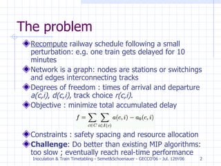
The document discusses using an inoculation approach to solve the problem of rescheduling railway trains following a small perturbation like a delay. The inoculation approach involves first running the algorithm with an "empty" incident to solve initial constraints and find a reasonable starting permutation, then using that solution to initialize the population for solving the actual problem. Experimental results show the inoculation approach finds good solutions faster than alternatives for both easy and hard instances of the scheduling problem.

1. On the Effects of Inoculation: an Example in Train Scheduling Y. Semet * , M. Schoenauer INRIA Orsay, France Research funded by SNCF *:now with EUROBIOS (complexity science for business problems)

2. The problem Recompute railway schedule following a small perturbation: e.g. one train gets delayed for 10 minutes Network is a graph: nodes are stations or switchings and edges interconnecting tracks Degrees of freedom : times of arrival and departure a(c,i) , d(c,i) , track choice r(c,i) . Objective : minimize total accumulated delay Constraints : safety spacing and resource allocation Challenge : Do better than existing MIP algorithms: too slow ; eventually reach real-time performance

3. Zoom in: one node…

4. Zoom out: Space/Time Diagrams A global overview of the railway network Visual representation of the phenotype Helps to graphically visualize constraints

5. Initial times Stopping times Safety spacing in both tracks and nodes Connecting trains Inter-routes shared resources conflicts: heart of the problem’s combinatorial difficulty Constraints

6. How to solve it ? Using an indirect approach. Widely used in Evolutionary Scheduling Direct approach impractical Indirect approach uses a mapping function: permutations + greedy scheduling heuristic [3 4 5 1 2 6 8 7] Scheduler Optimization plays with permutations

7. Scheduler outline For each train c ( following the permutation) For each Node i (in order) For each route r Initialize a and d (theoretical values) While (conflict) delay a and d or “ kick” obstacles Pick route yielding earliest d (greediness) Important: semi-greedy instead of actually greedy: optimality is enforced only at the node level, not at the train level

8. Solving conflicts: moving forward in time i Space Time j Train c’ is already scheduled Train c is being scheduled Safety spacing threshold a(c,j) : violation !! α α

9. Solving conflicts: moving forward in time i Space Time j Train c’ is already scheduled Train c is being scheduled Safety spacing threshold a(c,j) α α

10. Solving conflicts: “kicking” obstacles out i Space Time j Train c’ is already scheduled Train c is being scheduled α α

11. Solving conflicts : “kicking” obstacles out i Space Time j Train c is being scheduled α α Kick !

12. Solving conflicts : “kicking” obstacles out i Space Time j Train c is being scheduled

13. Solving conflicts : “kicking” obstacles out i Space Time j Train c is now scheduled Train c’ is being re-scheduled

14. Global picture : a ( μ + λ ) scheme + μ parents Keep μ best individuals λ offspring Sélection = [3 4 5 1 2 6 8 7]

15. Global picture : a ( μ + λ ) scheme + μ parents Keep μ best individuals λ offspring Sélection = [3 4 5 1 2 6 8 7]

16. The Swap Mutation Swapping 2 close by elements ( d < R ), T times T realization of a binomial law Calibrated decrease ( cf. simulated annealing ) [ 1 4 3 2 5 6 7 8 ] [ 1 2 3 4 5 6 7 8 ] R

17. Inoculation : The Art of the Start Initialization : an excellent way to provide the GA with relevant problem knowledge 3 problems in 1 for the GA : Fixing initial constraint violations Finding a reasonable starting permutation The actual problem The Idea : Solving 1. and 2. once and for all How : running the algorithm once with an “empty” incident (with delay=0) Solving 3. : Initialize population around the best permutation obtained (the Inoculant I 0 )

18. A large and complex problem 541 trains, several 100s nodes 1 million variables 3 millions constraints e.g. : 1 train delayed for 10 minutes inside a large connecting node (gare St-Lazare in Paris) Scheduling takes 1s per individual on average Results average over 11 runs Comparisons (GA, CPLEX, GA+CPLEX) over 24 hours

19. Algorithmic Settings & Experiments GA parameters: (10+70 scheme) Evolutionary Programming Tournament Ordered Selection R=12 Inoculation Variants Mass Mutation Gradual Perturbation Layer Initialization Experimental plan: 2 choices related wrt exploration/exploitation Which Inoculation variant ? Constant mutation rate or not ? Results : Easy Instances : Layers + decreasing rate Hard Ones : Mass Mutation + constant rate

20. The Benefits of Inoculation Easy Instances

21. The Benefits of Inoculation Hard Instances

22. The Benefits of Inoculation Hard Instances

23. Conclusions Drawback: a lot of time and efforts as well as large expert knowledge required to design the scheduler : not easy to adapt to other contexts/problems But a clear success for this problem: Natural formulation : usable for decision support Efficiency : good solutions quickly Inoculation: from tie/defeat to victory vs. CPLEX 1 minute of delay = 1000 $ 1 incident in 1 city per day = 21.9 million dollars yearly potential savings And, if parallelized, not so far from real-time use {semet,marc}@lri.fr