Download as PDF, PPTX

![Background 9
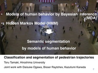
¡ Trajectory prediction
¡ Abnormal behavior detection ¡ Crowd behavior analysis
[Zhou+, IJCV2015] [Lee+,CVPR2017]
[Saligrama+,CVPR2012] [Solmaz+,PAMI2012]
¡ Trajectory classification](https://image.slidesharecdn.com/20180302talkslidebitspilani-180321152633/85/Semantic-segmentation-of-trajectories-with-agent-models-3-320.jpg)
![Related work
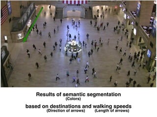
¡ TRAOD [Lee+, ICDE2008]
¡ Trajectory outlier detection
¡ Segmentation by MDL as preprocessing
¡ Transportation Mode [Zheng+, ACM WWW2008]
¡ Estimation of Transportation Mode (Walk, Car Bus, Bike)
from GPS data
¡ Semantic segmentation based on Transportation Mode
10
No segmentation methods
based on human behavior
(Minimum Description Length)](https://image.slidesharecdn.com/20180302talkslidebitspilani-180321152633/85/Semantic-segmentation-of-trajectories-with-agent-models-4-320.jpg)
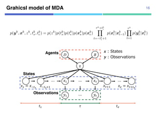
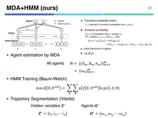
![Proposed method (MDA+HMM)
¡ Extend classification method to semantic segmentation
by combining with Hidden Markov Model
11
Models of human behavior (or agents) Parameter estimation
Pedestrian trajectory Semantic segmentation
MDA+HMM
MDA
[Zhou+, IJCV2015]
HMM
[Baum, 1972]
[Viterbi, 1967]
!" !# !$ !% !& !' !()# !()" !(⋯
+" +# +,
-" -# -,⋯
. /Agents
Observations
0" 0# 0,⋯
States
1
2
3
4](https://image.slidesharecdn.com/20180302talkslidebitspilani-180321152633/85/Semantic-segmentation-of-trajectories-with-agent-models-5-320.jpg)
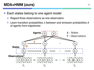
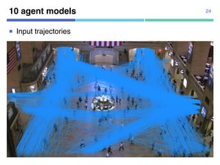
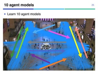
![MDA: Mixture model of Dynamic pedestrian-Agents
¡ Example : Input trajectories (blue) and two agent models
12
[Zhou+, IJCV2015]](https://image.slidesharecdn.com/20180302talkslidebitspilani-180321152633/85/Semantic-segmentation-of-trajectories-with-agent-models-6-320.jpg)
![MDA (Mixture model of Dynamic pedestrian-Agents)
¡ Initialize LDS and Gaussian distributions
13
start
goal
start goalD
D
[Zhou+, IJCV2015]
B
B
B
B
Agents have D and B respectively
• D (dynamics) : Linear dynamic system
• B (belief) : Gaussian distributions
(start, goal)](https://image.slidesharecdn.com/20180302talkslidebitspilani-180321152633/85/Semantic-segmentation-of-trajectories-with-agent-models-7-320.jpg)
![MDA (Mixture model of Dynamic pedestrian-Agents)
¡ Learn agents by EM algorithm
14
start
goal
goal
start D
D
[Zhou+, IJCV2015]
B
B
B
B
Agents have D and B respectively
• D (dynamics) : Linear dynamic system
• B (belief) : Gaussian distributions
(start, goal)](https://image.slidesharecdn.com/20180302talkslidebitspilani-180321152633/85/Semantic-segmentation-of-trajectories-with-agent-models-8-320.jpg)
![Dynamics and Beliefs
¡ belief parameter
15
! = ($, &, ', () : dynamics
* = (+,, Φ,, +., Φ.): belief
/
0
(!, *, 1) : Agent model
1 : Weights
!"
!#
missing missingobserved$%
$&
'%~)($%, Φ%)
'&~)($&, Φ&)
$%
$&
.
Kalman filter + Kalman smoother
¡ dynamics parameter
!"#$
%"
Observation !"~'(!"|%")
= ,(!"|%", .)
State
!"#$
%!"#$ + '
!"~) !" !"#$
= +(!"|%!"#$ + ., 0)
*( ⋯ *)
ervations
/ 0-
Figure 1. State space model of MDA [9]
the sequence of states x except xs and xe. Figure 1 shows the state
= {yk} MDA estimates M agents ⇥ = {(Dm, Bm, ⇡m)} by maximizing
ood;
L =
X
k
log p(yk
, xk
, zk
, tk
s , tk
e|⇥), (6)
Hereafter, x1:T denotes the sequence of states x except xs and xe. Figure 1 shows the
pace model of MDA.
.2 Learning
Given K trajectories Y = {yk} MDA estimates M agents ⇥ = {(Dm, Bm, ⇡m)} by maxim
he following log likelihood;
L =
X
k
log p(yk
, xk
, zk
, tk
s , tk
e |⇥),
where the joint probability is given by
p(yk
, xk
, zk
, tk
s , tk
e ) = p(zk
)p(tk
s )p(tk
e )p(xk
s )p(xk
e )
⌧k
+tk
eY
t= tk
s +1
p(xk
t |xk
t 1)
⌧k
Y
t=1
p(yk
t |xk
t )
with respect to parameters ⇥.
This can be rewritten by replacing hidden variables H = {hk}, hk = {zk, tk
s , tk
e } as follow
¡ Joint distribution of trajectory k
¡ Log likelihood for k trajectories
3.2 Learning
Given K trajectories Y = {yk} MDA estimates M agents ⇥ = {(Dm, Bm, ⇡m)} by ma
the following log likelihood;
L =
X
k
log p(yk
, xk
, zk
, tk
s , tk
e |⇥),
where the joint probability is given by
p(yk
, xk
, zk
, tk
s , tk
e ) = p(zk
)p(tk
s )p(tk
e )p(xk
s )p(xk
e )
⌧k
+tk
eY
t= tk
s +1
p(xk
t |xk
t 1)
⌧k
Y
t=1
p(yk
t |xk
t )
with respect to parameters ⇥.
This can be rewritten by replacing hidden variables H = {hk}, hk = {zk, tk
s , tk
e } as fo
L =
X
k
log p(yk
, xk
, hk
|⇥)
Hereafter, x1:T denotes the sequence of states x except xs and xe. Figure 1 shows
space model of MDA.
3.2 Learning
Given K trajectories Y = {yk} MDA estimates M agents ⇥ = {(Dm, Bm, ⇡m)} by ma
the following log likelihood;
L =
X
k
log p(yk
, xk
, zk
, tk
s , tk
e |⇥),
where the joint probability is given by
p(yk
, xk
, zk
, tk
s , tk
e ) = p(zk
)p(tk
s )p(tk
e )p(xk
s )p(xk
e )
⌧k
+tk
eY
t= tk
s +1
p(xk
t |xk
t 1)
⌧k
Y
t=1
p(yk
t |xk
t )
with respect to parameters ⇥.
This can be rewritten by replacing hidden variables H = {hk}, hk = {zk, tk
s , tk
e } as fo
Hidden variables](https://image.slidesharecdn.com/20180302talkslidebitspilani-180321152633/85/Semantic-segmentation-of-trajectories-with-agent-models-9-320.jpg)
![EM algorithm for MDA 17
¡ EM algorithm
max $ = &
'
log +(-'|/', ℎ', 2)
ℎ' = {5', 67
', 68
'}
:2∗ = arg =>?@A 2, :2
¡ E step
¡ M step
3.2.1 E step of original MDA
Q(⇥, ˆ⇥) = EX,H|Y,ˆ⇥[L]
= EH|Y,ˆ⇥[EX|Y,H,ˆ⇥[L]]
=
X
k
X
hk
k
Exk|yk,hk [log p(yk
, xk
, hk
|⇥)]
=
X
k
X
hk
k
log p(yk
, ˆxk
, hk
|⇥),
where ˆxk
= Exk|yk,hk [xk] is computed by the modified Kalman filter [9, 12
Weights k are posterior probabilities given as follows;
k
= p(hk
|yk
, ˆ⇥)
=
p(hk|ˆ⇥)p(yk|hk, ˆ⇥)
p(yk|ˆ⇥)
By further assuming the independence among hidden variables z, t , t , w
Q(⇥, ˆ⇥) = EX,H|Y,ˆ⇥[L]
= EH|Y,ˆ⇥[EX|Y,H,ˆ⇥[L]]
=
X
k
X
hk
k
Exk|yk,hk [log p(yk
, xk
, hk
|⇥)]
=
X
k
X
hk
k
log p(yk
, ˆxk
, hk
|⇥),
where ˆxk
= Exk|yk,hk [xk] is computed by the modified Kalman filter [9, 12].
Weights k are posterior probabilities given as follows;
k
= p(hk
|yk
, ˆ⇥)
=
p(hk|ˆ⇥)p(yk|hk, ˆ⇥)
p(yk|ˆ⇥)
By further assuming the independence among hidden variables z, ts, te, we have
p(hk
|ˆ⇥) = p(zk
, tk
s , tk
e|ˆ⇥) = p(zk
|ˆ⇥)p(tk
s |ˆ⇥)p(tk
e|ˆ⇥)
=
X
k
X
hk
k
log p(yk
, ˆxk
, hk
|⇥),
where ˆxk
= Exk|yk,hk [xk] is computed by the modified Kalman filter [9, 12].
Weights k are posterior probabilities given as follows;
k
= p(hk
|yk
, ˆ⇥)
=
p(hk|ˆ⇥)p(yk|hk, ˆ⇥)
p(yk|ˆ⇥)
By further assuming the independence among hidden variables z, ts, te, we have
p(hk
|ˆ⇥) = p(zk
, tk
s , tk
e |ˆ⇥) = p(zk
|ˆ⇥)p(tk
s |ˆ⇥)p(tk
e |ˆ⇥)
By removing ts, te by assuming those be uniform, we have
k
=
p(zk|ˆ⇥)p(yk|hk, ˆ⇥)
P
hk p(zk|ˆ⇥)p(yk|hk, ˆ⇥)
where likelihood p(yk|hk, ˆ⇥) is also computed by the modified Kalman filter [9, 12].
Kalman filter
3.2.1 E step of original M
Q(⇥
where ˆxk
= Exk|yk,hk [xk] i
Weights k are posterior
Weights](https://image.slidesharecdn.com/20180302talkslidebitspilani-180321152633/85/Semantic-segmentation-of-trajectories-with-agent-models-11-320.jpg)
![Issue of MDA 19
¡ One trajectory is represented by one agent model
¡ Cannot switch agent models in one trajectory
[Zhou+, IJCV2015]
D B
z
"# = "%&'
"( ")
*( ⋯
⋯⋯
*)
"%&',( "),(
⋯
"- = "),&.
Agents
States
Observations
/0# 0-
1
2](https://image.slidesharecdn.com/20180302talkslidebitspilani-180321152633/85/Semantic-segmentation-of-trajectories-with-agent-models-12-320.jpg)
![Related model : Switching Kalman Filter
¡ Can estimate agents !" in time series
¡ Transition probabilities between agent models are required
20
Observations
States
Agents z" z#$"z% z# z#&"⋯ ⋯
(" (#$"(% (# (#&"
)" )#$")% )# )#&"
⋯ ⋯
[Murphy, 1998]](https://image.slidesharecdn.com/20180302talkslidebitspilani-180321152633/85/Semantic-segmentation-of-trajectories-with-agent-models-13-320.jpg)
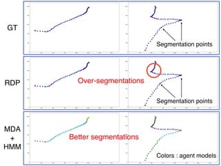
![¡ Real data
¡ 104 trajectories from “Pedestrian
Walking Path Dataset”
¡ Annotated segmentation points
manually
¡ 1920x1080 pixels
¡ 4-fold cross validation
Datasets
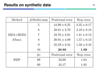
¡ Synthetic data
¡ Using 10 agent models
¡ Uniform transition probabilities
¡ 10,000 trajectories for estimation,
10,000 trajectories for test
¡ 1920x1080 pixels
23
[Yi+, CVPR2015]](https://image.slidesharecdn.com/20180302talkslidebitspilani-180321152633/85/Semantic-segmentation-of-trajectories-with-agent-models-16-320.jpg)
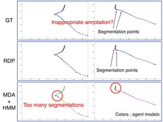
![¡ Real data
¡ 104 trajectories from “Pedestrian
Walking Path Dataset”
¡ Annotated segmentation points
manually
¡ 1920x1080 pixels
¡ 4-fold cross validation
Datasets
¡ Synthetic data
¡ Using 10 agent models
¡ Uniform transition probabilities
¡ 10,000 trajectories for estimation,
10,000 trajectories for test
¡ 1920x1080 pixels
32
[Yi+, CVPR2015]](https://image.slidesharecdn.com/20180302talkslidebitspilani-180321152633/85/Semantic-segmentation-of-trajectories-with-agent-models-25-320.jpg)
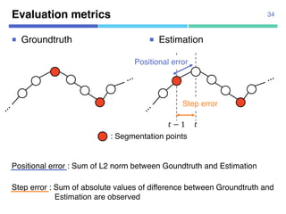
![Baseline 33
¡ Ramer-Douglas-Peucker (RDP) algorithm
¡ Trajectory simplification with parameter !
¡ Segmentation with keeping trajectory’s shape
¡ Appropriate ! setting is required
¡ No estimation of agent models
Wikipedia, “Ramer–Douglas–Peucker algorithm”
[Ramer, 1972] [Douglas+, 1973]](https://image.slidesharecdn.com/20180302talkslidebitspilani-180321152633/85/Semantic-segmentation-of-trajectories-with-agent-models-26-320.jpg)
![¡ Real data
¡ 104 trajectories from “Pedestrian
Walking Path Dataset”
¡ Annotated segmentation points
manually
¡ 1920x1080 pixels
¡ 4-fold cross validation
Datasets
¡ Synthetic data
¡ Using 10 agent models
¡ Uniform transition probabilities
¡ 10,000 trajectories for estimation,
10,000 trajectories for test
¡ 1920x1080 pixels
35
[Yi+, CVPR2015]](https://image.slidesharecdn.com/20180302talkslidebitspilani-180321152633/85/Semantic-segmentation-of-trajectories-with-agent-models-28-320.jpg)
![¡ Real data
¡ 104 trajectories from “Pedestrian
Walking Path Dataset”
¡ Annotated segmentation points
manually
¡ 1920x1080 pixels
¡ 4-fold cross validation
Datasets
¡ Synthetic data
¡ Using 10 agent models
¡ Uniform transition probabilities
¡ 10,000 trajectories for estimation,
10,000 trajectories for test
¡ 1920x1080 pixels
37
[Yi+, CVPR2015]](https://image.slidesharecdn.com/20180302talkslidebitspilani-180321152633/85/Semantic-segmentation-of-trajectories-with-agent-models-30-320.jpg)
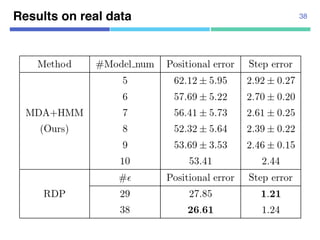
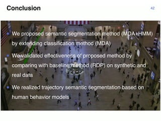

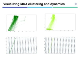
This document discusses a semantic segmentation method for pedestrian trajectories using a combination of Mixture Model of Dynamic pedestrian Agents (MDA) and Hidden Markov Models (HMM). It focuses on enhancing trajectory classification by integrating human behavior models and evaluating its effectiveness against traditional methods. Results indicate improved segmentation accuracy on both synthetic and real datasets compared to baseline techniques.


![Getting Started with Apache Spark: Big Data Made Simple [Free Meetup]](https://cdn.slidesharecdn.com/ss_thumbnails/apachesparkgettingstarted-260203175547-8361bcc3-thumbnail.jpg?width=640&height=640&fit=bounds)


