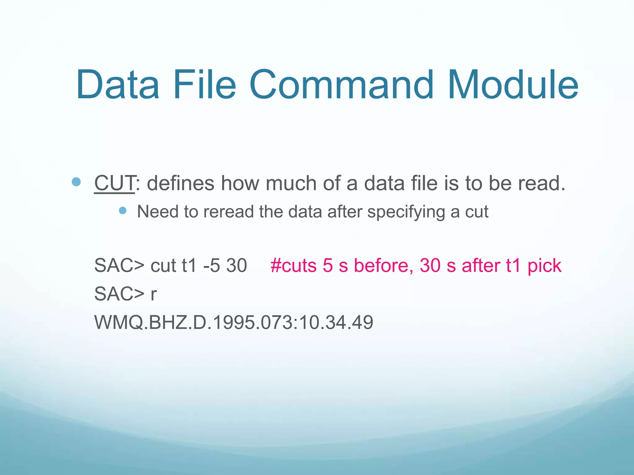
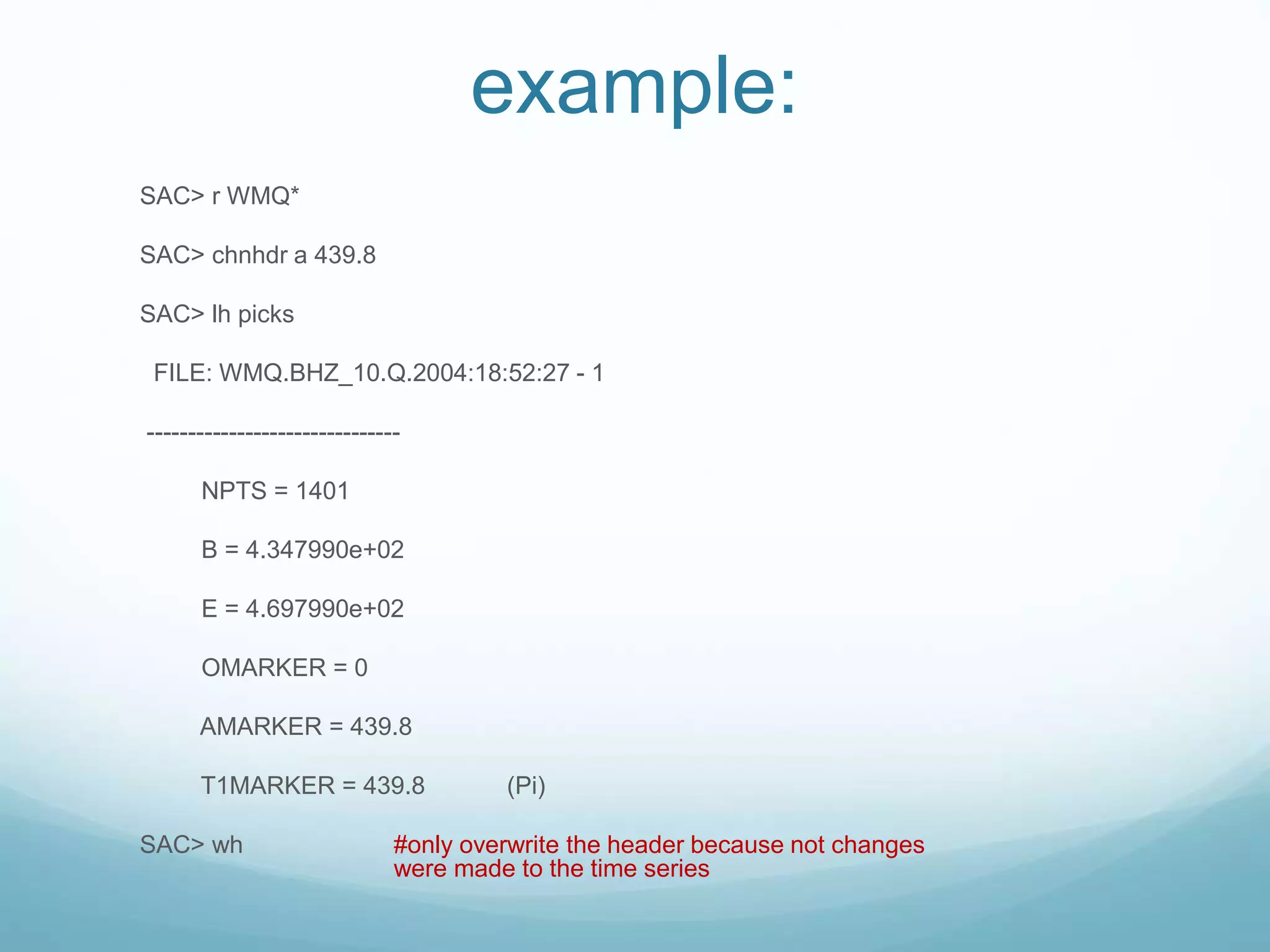
SAC (Seismic Analysis Code) is a command-driven program developed in the 1980s for manipulating seismological time series data. It allows users to interactively read seismic data, perform processing like filtering and phase picking, and create publication-quality plots. SAC can read various data formats and stores seismic signal information and processing results in customizable headers associated with each file.

2. Seismic Analysis Code
(SAC)
Basic Data Manipulation

3. SAC
 Seismic Analysis Code was developed at Lawrence
Livermore National Laboratory and University of California in
the early 1980's.
 It is a command-driven program generally implemented on
many types of UNIX operating systems and has become a
standard data manipulation tool in seismology.
 Its binary data format is one of the principle data formats
used today in storing and manipulating seismological time
series data.

4.  SAC was designed as an aid to research seismologists in
the study of seismic events. As such, it is used for quick
preliminary analyses, for routine processing, for testing new
techniques, for detailed research, and for creating
publication quality graphics.
ceri% sac
SEISMIC ANALYSIS CODE [09/04/2008 (Version 101.2)]
Copyright 1995 Regents of the University of California
SAC>

5. What can it do?
 Interactively read seismogram data
 Perform many standard data processing operations, such as
 Filtering
 Time picks
 Amplitude picks
 Correlation
 Fourier transforms
 Seismic instrument corrections
 Particle motion rotation
 Trace envelopes
 Spectral ratios
 Linear regressions
 Frequency-wavenumber analysis
 Create a variety of plots of the data and resulting analysis

6. SAC’s competitors (analysis)
 Various versions of DATASCOPE (now Antelope)
 MATSEIS/Coral other Matlab based programs
 SEISAN
 XPICK
 Seismic UNIX
- others

7. SAC’s competitors
(data format)
 SEED (Standard for the Exchange of Earthquake Data)
 SEISAN (widely used in Central and South America/Europe)
 CSS (Center for Seismic Studies, associated with treaty verification)
 SUDS (Seismic Unified Data System, from Willie Lee PC based
system/USGS)
 SEG-Y (the standard for seismic reflection data)
 AH (Ad Hoc, pre-SEED shows up from AVO/HVO, etc. in archives)
 Others (new ones crop up every 5-10 years to address the chaotic state of
affairs.)

8. Commands
 SAC commands fall into three main categories
 Parameter-setting: change values of internal SAC
parameters
 Action-producing: perform some operation on the signals
currently in selected memory based upon the values of
these parameters
 Data-set: determine which files are in active (selected)
memory and therefore will be acted upon

9. Commands
 HELP calls up a list of all commands
 help command can be used to view manual pages

10. Defaults
 In order to make SAC quick to learn and easy to use,
default values for all operational parameters were
carefully chosen.
 At the same time, almost all of these parameters are
under direct user control.
 SAC can be reinitialized to this default state at any
time by executing the INICM command.

11. Data Format and Header
 Each signal or seismogram is stored in a separate binary
or alphanumeric data file.
 SAC can read data in a variety of formats:
 SAC Binary Format (most common)
 CSS format
 SDD format
 ASCII formats
 Each data file contains a header that describes the
contents of that file.

12. listhdr (lh): lists the
headers of the files in
memory.
SAC> listhdr
FILE: ccm_sumatra_.bhe - 1
----------------------
NPTS = 389396
B = 0.000000e+00
E = 1.946975e+04
IFTYPE = TIME SERIES FILE
LEVEN = TRUE
DELTA = 5.000000e-02
IDEP = UNKNOWN
DEPMIN = -1.073057e+06
DEPMAX = 1.091875e+06
DEPMEN = 8.429739e+02
OMARKER = 7.315 (origin )
KZDATE = DEC 26 (361), 2004
KZTIME = 01:09:52.684
IZTYPE = BEGIN TIME
KSTNM = CCM
CMPAZ = 9.000000e+01
CMPINC = 9.000000e+01
STLO = -9.124470e+01
DIST = 8.818225e+03
AZ = 1.854116e+02
BAZ = 2.013326e+02
LOVROK = TRUE
NVHDR = 6
LPSPOL = TRUE
LCALDA = TRUE
KCMPNM = BHE
KNETWK = US

13. Time
 The SAC header contains a reference or zero time, stored
as six integers (NZYEAR, NZJDAY, NZHOUR, NZMIN,
NZSEC, NZMSEC), but normally printed in an equivalent
alphanumeric format (KZDATE and KZTIME).
SAC> lh #list header
FILE: GRAT.EHZ.NM – 1 #this is a partial header
-----------------
NPTS = 360100
B = 0.000000e+00
E = 3.600990e+03
IFTYPE = TIME SERIES FILE
DELTA = 1.000000e-02
KZDATE = APR 06 (097), 2008
KZTIME = 02:59:59.320

14. Event and Station Info
 SAC header can store station and event info
SAC> lh
FILE: WMQ.BHZ.D.1995.073:10.34.49 - 1
---------------------------------
KSTNM = WMQ
STLA = 4.382110e+01
STLO = 8.769500e+01
STEL = 8.970000e+02
EVLA = 3.086000e+00
EVLO = 9.584800e+01
EVDP = 3.040000e+01

15.  Once the event and station information are store, the
program automatically calculates and stores distance (km),
azimuth (degrees), backazimuth (degrees), and great circle
arc length (degrees)
DIST = 4.583862e+03
AZ = 3.510350e+02
BAZ = 1.675856e+02
GCARC = 4.120298e+01

16. Phase Info
 SAC can be used to pick and store phase information in
header variables A & T0-T9. The Omarker is reserved to for
the origin time. All pick and origin times are stored in secs
from the zero time of the file.
OMARKER = 0
AMARKER #not set in this example
T0MARKER #not set in this example
T1MARKER = 462.7 (P)
T2MARKER = 834.76 (S)
T4MARKER = 472.5 (pP)
T6MARKER = 478 (sP)

17. Data File Command Module
 This module is used to read, write, and access SAC
data files.
 READ (r): reads data files from disk into memory
SAC> r *.SAC #read any files that end in .SAC
Uses standard UNIX wildcards: reads all files
whose filenames end in “.SAC”

18. Data File Command Module
 WRITE (w): writes the data currently in memory to
disk
 You can write manipulated data into a range of file formats
or simply overwrite the current set of files (so be careful,
you have been warned!)

19. Let’s try it (and also jump ahead to graphics
action module to plot (“p”) it) –
% sac
SEISMIC ANALYSIS CODE [8/8/2001 (Version 00.59.44)]
Copyright 1995 Regents of the University of California
SAC> read ccm_sumatra_.bhz
SAC> plot

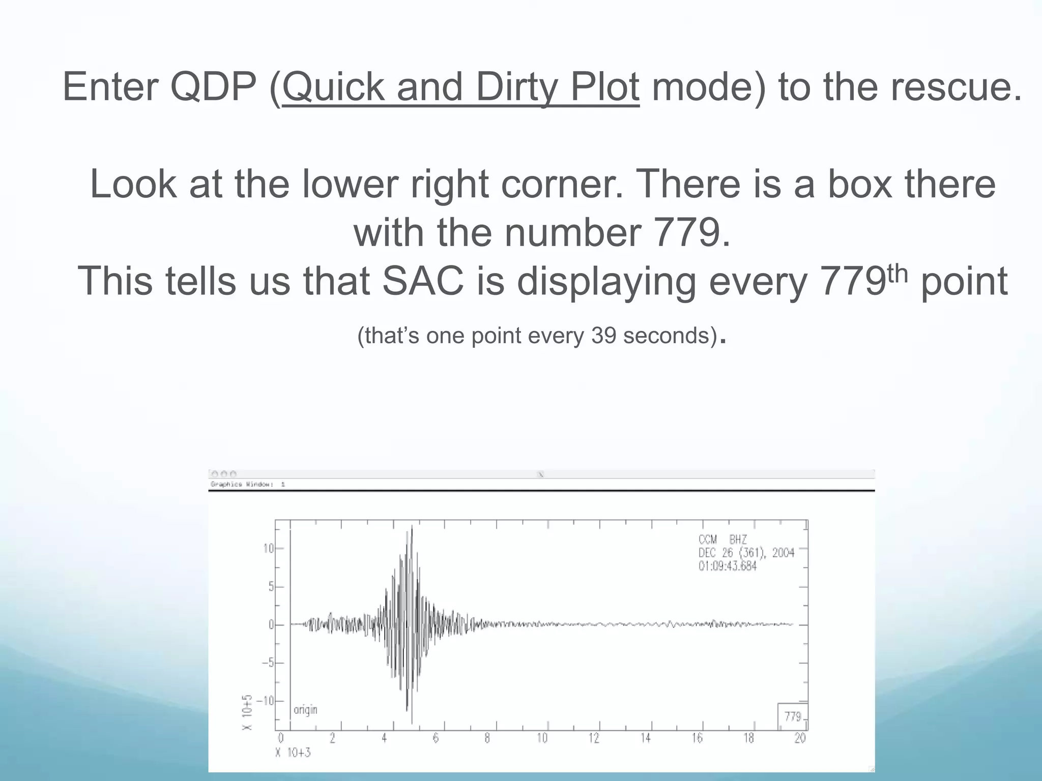
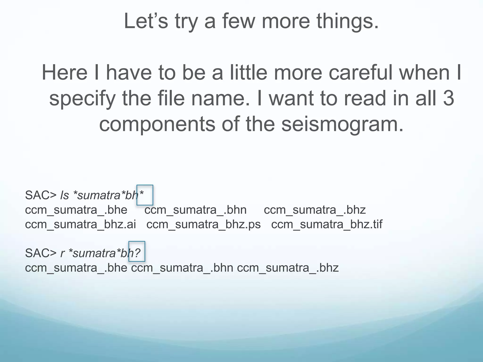
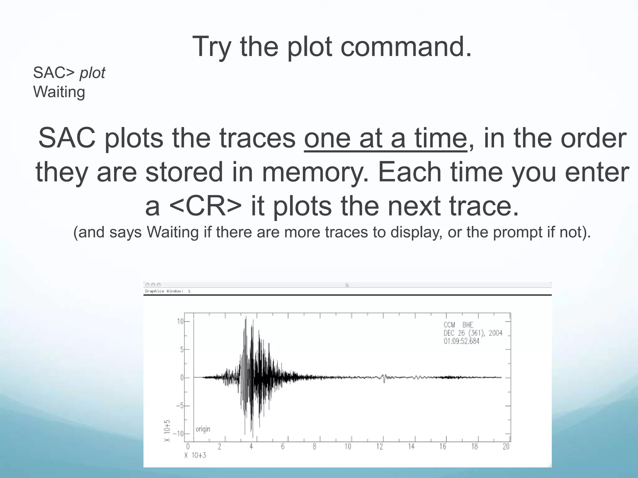
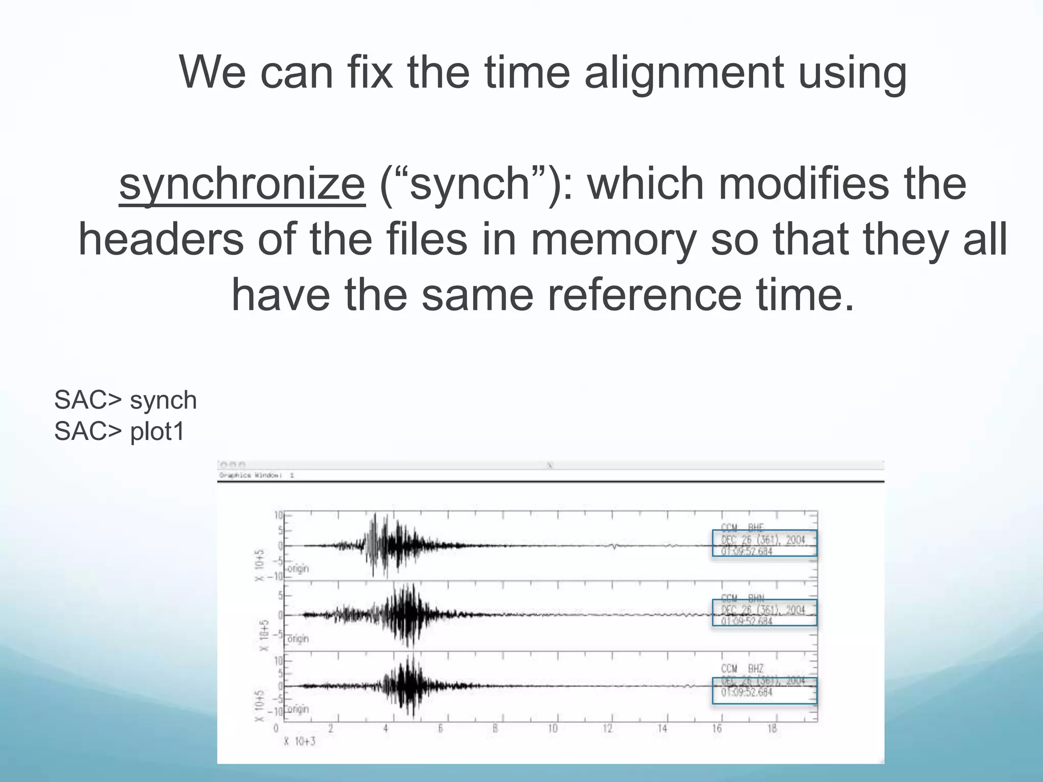
20. Let’s try it (and also jump ahead to graphics
action module to plot (“p”) it) –
% sac
SEISMIC ANALYSIS CODE [09/04/2008 (Version 101.2)]
Copyright 1995 Regents of the University of California
SAC> read ccm_sumatra_.bhz
SAC> plot

21. This seismogram is 20,000 seconds long, with
samples 20 times per second.
It has over 3,890,000 points and would take almost an
hour to draw at 9600 baud, which was the rate of
computers when SAC originally written.

22. Enter QDP (Quick and Dirty Plot mode) to the rescue.
Look at the lower right corner. There is a box there
with the number 779.
This tells us that SAC is displaying every 779th point
(that’s one point every 39 seconds).

23. Since we are on a modern computer we can afford to
plot all the data
So we turn the QDP “feature” off
SAC> qdp off
SAC> plot
This plot is now “good”.

24. • So far there is one file in memory. If we simply read in
another one – it will clobber what we have there.
• If we need to read in more data (say we have processed the
data we’ve read in and now want a spectral ratio of the
processed data with the original data) we have to use the
“more” option to read in the additional data.
SAC>read more filename

25. • In general SAC does commands to all the files in
memory.
• If the command is starting from scratch (like a read)
it clobbers what is already there.
• Some commands require certain pairs of files

26. Let’s try a few more things.
Here I have to be a little more careful when I
specify the file name. I want to read in all 3
components of the seismogram.
SAC> ls *sumatra*bh*
ccm_sumatra_.bhe ccm_sumatra_.bhn ccm_sumatra_.bhz
ccm_sumatra_bhz.ai ccm_sumatra_bhz.ps ccm_sumatra_bhz.tif
SAC> r *sumatra*bh?
ccm_sumatra_.bhe ccm_sumatra_.bhn ccm_sumatra_.bhz

27. Try the plot command.
SAC> plot
Waiting
SAC plots the traces one at a time, in the order
they are stored in memory. Each time you enter
a <CR> it plots the next trace.
(and says Waiting if there are more traces to display, or the prompt if not).

28. New command – plot1 ( “p1”).
SAC> plot1
SAC>
This command plots all the data in memory on
one plot.

29. Say I want to process these three traces
together.
Notice that the three traces do not start at the
same time (and we will see that they are not
the same lengths, either).

30. We can fix the time alignment using
synchronize (“synch”): which modifies the
headers of the files in memory so that they all
have the same reference time.
SAC> synch
SAC> plot1

31. FILE: ccm_sumatra_.bhe – 1
NPTS = 389396
B = 0.000000e+00
KZDATE = DEC 26 (361), 2004
KZTIME = 01:09:52.684
FILE: ccm_sumatra_.bhn – 2
NPTS = 389328
B = 0.000000e+00
KZDATE = DEC 26 (361), 2004
KZTIME = 01:09:48.485
FILE: ccm_sumatra_.bhz – 3
NPTS = 389600
B = 0.000000e+00
KZDATE = DEC 26 (361), 2004
KZTIME = 01:09:43.684
B = 0.000000e+00
KZDATE = DEC 26 (361), 2004
KZTIME = 01:09:52.684
B = -4.199000e+00
KZDATE = DEC 26 (361), 2004
KZTIME = 01:09:52.684
B = -9.000000e+00
KZDATE = DEC 26 (361), 2004
KZTIME = 01:09:52.684
Before synch After synch

32.  CUT: defines how much of a data file is to be read.
 Need to reread the data after specifying a cut
SAC> cut t1 -5 30 #cuts 5 s before, 30 s after t1 pick
SAC> r
WMQ.BHZ.D.1995.073:10.34.49
Data File Command Module

33.  READHDR (rh) and WRITEHDR (wh): read and write
headers without the data
 LISTHDR (lh): list the header contents
 CHNHDR: change header values
 COPYHDR: copy header values from one file to the
others in memory

34. example:
SAC> r WMQ*
SAC> chnhdr a 439.8
SAC> lh picks
FILE: WMQ.BHZ_10.Q.2004:18:52:27 - 1
-------------------------------
NPTS = 1401
B = 4.347990e+02
E = 4.697990e+02
OMARKER = 0
AMARKER = 439.8
T1MARKER = 439.8 (Pi)
SAC> wh #only overwrite the header because not changes
were made to the time series

35. Graphics Action Module
 PLOT (p): plots each signal in memory on a separate
plot.
 PLOT1 (p1): plots a set of signals on a single plot with
a common x axis and separate y axes.
 PLOT2 (p2): plots a set of signals on a single plot with
common x and y axes (i.e. an overlay plot).

36. SAC> r WMQ* AAK*
WMQ.BHZ_10.Q.2004:18:52:27 AAK.BHZ_00.Q.2004:18:52:53
SAC> r more BJT*
BJT.BHZ_00.Q.2004:18:50:19
SAC> plot
Waiting
Waiting

37. SAC> p1
SAC> p1 rel

38. SAC> color on increment on
SAC> p2
SAC> p2 rel

39. Graphics
 There are three graphics ``devices'' currently
supported.
 SGF is a general purpose device driver representing a
large class of actual physical devices.
 XWINDOWS is a general windowing system running on
most high-resolution, bit-mapped graphics workstations.
 SUNWINDOW, is a windowing system that was available
on the Sun in SunOS 4.X.

40. Xwindows or X
 X is widely used on the graphics workstation and
offers one of the best frameworks for developing
portable window-based applications.
 Should be the default graphics device.
 Can be turned on using the begin device (bg)
command
sac> bd x

41. SGF (SAC Graphics File)
 SAC Graphics File contains all the information
needed to generate a single plot on any graphics
device.
 Each plot is stored in a separate file. The file names
are of the form ``Fnnn.SGF'' where ``nnn'' is the plot
number, beginning with ``001''.
 Can be turned on using
sac> bd sgf

42.  To create a postscript plot, you would turn on the sgf
device, create your plot, and then run a conversion
program called sgftops
SAC> bd sgf
SAC> p1 rel #plot waveform to file f001.sgf
SAC> sgftops f001.ps newplot.ps
SAC> ls newplot.ps
newplot.ps
SAC> bd x #or ed sgf