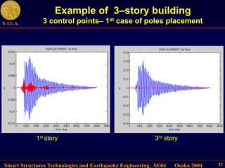
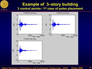
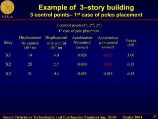
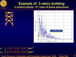
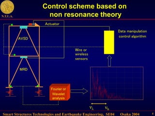
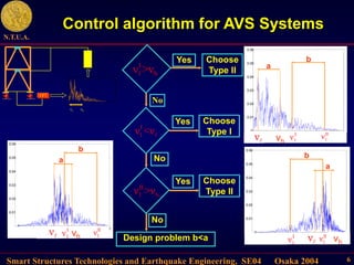
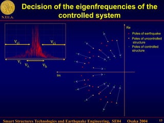
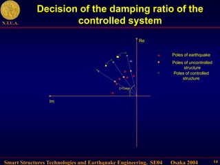
This document describes control algorithms for mitigating seismic hazard in structures. It presents strategies for placing the poles of a controlled structure based on the frequency content of an incoming earthquake. Algorithms are proposed for active variable stiffness systems and variable damping systems using pole placement and sliding mode control. Examples applying these algorithms to 3-story and 8-story buildings show reductions in displacement, acceleration, and forces compared to uncontrolled structures.

1. Control algorithms for mitigating seismic hazard
in structures accounting for the incoming
earthquake’s frequency content
National Technical University of Athens
School of Civil Engineering
Metal Structures Laboratory
Nikos Pnevmatikos, Charis Gantes
Smart Structures Technologies and
Earthquake Engineering (SE04)
July 6-9, 2004
Osaka, Japan

2. Smart Structures Technologies and Earthquake Engineering, SE04 Osaka 2004
N.T.U.A.
2
Contents
• Control strategy based on non resonance theory
• Examples: 3–story and 8-story building
• Pole placement algorithm based on the frequency
content of the incoming earthquake signal
• Algorithm for active variable stiffness system
• Sliding mode control and pole placement

3. Smart Structures Technologies and Earthquake Engineering, SE04 Osaka 2004
N.T.U.A.
4
Control scheme based on
non resonance theory
νl νh
Fourier or
Wavelet
analysis
AVSD
MRD
Data manipulation
control algorithm
Wire or
wireless
sensors
Actuator

4. Smart Structures Technologies and Earthquake Engineering, SE04 Osaka 2004
N.T.U.A.
5
Active variable stiffness system
AVSD
braces
• Frequency content of the
earthquake signal is obtained via
on line FFT process
FFT
Algorithm for
AVS systems
• Based on the main frequencies
and their range a control algorithm
decides which stiffness type will be
chosen. Type I (braces off), Type II
(braces on)

5. Smart Structures Technologies and Earthquake Engineering, SE04 Osaka 2004
N.T.U.A.
6
Control algorithm for AVS Systems
FFT
νl νh
Design problem b<a
No
No
0 1 2 3 4 5 6 7
0
0.01
0.02
0.03
0.04
0.05
0.06
a
νh
b
I
1
ν II
1
ν
II
1 h
ν >ν
Yes Choose
Type II
ν
0 1 2 3 4 5 6 7
0
0.01
0.02
0.03
0.04
0.05
0.06
a
νh
Yes Choose
Type II
I
1 h
ν >ν
b
I
1
ν
II
1
ν
ν
No
I
1
ν <ν
Yes Choose
Type I
0 1 2 3 4 5 6 7
0
0.01
0.02
0.03
0.04
0.05
0.06
a
νh
b
I
1
ν
II
1
ν
ν

6. Smart Structures Technologies and Earthquake Engineering, SE04 Osaka 2004
N.T.U.A.
7
MR Dampers or
Actuators
Pole placement algorithm based on the
frequency content of the incoming signal
Α, Β, λci
POLE
PLACEMENT =>
Kfm
νl, νh, =>
νci=κ νh,
ci i ci i
2
λ =ζ 2πν j 1-ζ

fm
f
f
1
f *
2
3
 
 
 
   
   
     
 
 
 
 
 
 
 
F K X
1
2
3
1
2
3
u
u
u
X
u
u
u
 
 
 
 
 
 
 
 
 
 
 
 
 
 
 

νl νh
FFT
Non linear behavior
Estimate the new Κ

7. Smart Structures Technologies and Earthquake Engineering, SE04 Osaka 2004
N.T.U.A.
10
Decision of the eigenfrequencies of the
controlled system
ci ci ci ci i
2
= 2π j2π
λ ζ ν 1-
ν ζ

2
i i i i i
λ =ζ 2πν j2πν 1-ζ
 ci ci
?, ?
ν ζ
 
i
2 2
i
i i
i
-ω =0 -ω =0
ω
2π
T = , ν =
ω 2π
2
   
 



T
n
T
n
n n
K M Φ K M
C Φ CΦ
M Φ MΦ
C M ω

g
- a
   
.. .
MU CU KU MΕ P
Uncontrolled
structure
   
fu fu f
U
= -
U
(t) t
 
   
 
F K K K X
f fu f fu g
( ) ( - a
   
.. .
B K B K
MU C- U K - )U MΕ P
g f
- a
    
.. .
MU CU KU Ε
Ε F
M P
Controlled
structure

8. Smart Structures Technologies and Earthquake Engineering, SE04 Osaka 2004
N.T.U.A.
11
Decision of the eigenfrequencies of the
controlled system
νl νh
νl, νh, => νci=κ νh,
ci i ci ci i
2
λ =ζ 2πν j2πν 1-ζ

νci=κ νh
νi structure eigenfreq. Re
Im
Poles of earthquake
Poles of uncontrolled
structure
Poles of controlled
structure

9. Smart Structures Technologies and Earthquake Engineering, SE04 Osaka 2004
N.T.U.A.
12
Decision of the eigenfrequencies of the
controlled system
νl νh
νi
Re
Im
νci=κ νh
Poles of earthquake
Poles of uncontrolled
structure
Poles of controlled
structure

10. Smart Structures Technologies and Earthquake Engineering, SE04 Osaka 2004
N.T.U.A.
13
Decision of the eigenfrequencies of the
controlled system
νl νh
νci νci
νi
Re
Im
Poles of earthquake
Poles of uncontrolled
structure
Poles of controlled
structure

11. Smart Structures Technologies and Earthquake Engineering, SE04 Osaka 2004
N.T.U.A.
14
Decision of the damping ratio of the
controlled system
Poles of earthquake
Poles of uncontrolled
structure
Re
Im
ξ=Cosφ
Poles of controlled
structure
ω

12. Smart Structures Technologies and Earthquake Engineering, SE04 Osaka 2004
N.T.U.A.
17
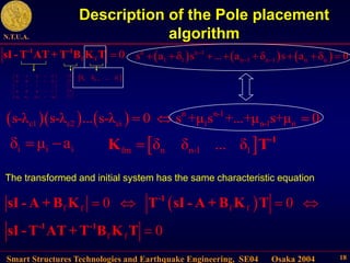
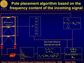
Description of the Pole placement
algorithm
.
f g g
ˆ ˆ F
  
-1 -1 -1 -1
p
X T ATX + T B T B a T B P
 
f f f
ˆ ˆ ˆ
- t -
 
F K X K TX = -K X
 
.
f f g g
ˆ ˆ
  
-1 -1 -1 -1
p
X T AT-T B K T X T B a T B P
Necessary and sufficient condition for arbitrary location of poles :
Controllability condition  2n-1
rank[ ... ]=2n
f f f
B AB A B
ˆ

X TX, T = SW
 n-1
=[ ... ]
f f f
S B AB A B
n 1 n 2 1
n 2 n 3
1
a a a 1
a a 1 0
a 1 0 0
1 0 0 0
 
 
 
 
 
 
 
 
 
 
W =
ai coefficients of the
characteristic
polynomial |sI-A|
.
f g g
   p
X AX+B F B a B P
f f 0

sI- A+B K
f
-

F K X

13. Smart Structures Technologies and Earthquake Engineering, SE04 Osaka 2004
N.T.U.A.
18
Description of the Pole placement
algorithm
     n n-1
c1 c2 ci 1 n-1 n
s-λ s-λ ... s-λ 0 s +μ s +...+μ s+μ 0
  
 
f f f f
f f
0 0
0
   

-1
-1 -1
sI - A + B K T sI - A + B K T
sI - T AT + T B K T
The transformed and initial system has the same characteristic equation
f f 0

-1 -1
sI - T AT + T B K T
n n 1 n 2 1
0 1 0 0
0 0 1 0
0 0 0 1
a a a a
 
 
 
 
 
 
 
 
   
 
0
0
0
1
 
 
 
 
 
 
 
 
 
n n 1 1
...

  
     
n n 1
1 1 n 1 n 1 n n
s a s ... a s a 0

 
       
i i i
μ a
    
fm n n-1 1
δ δ ... δ
 -1
K T

14. Smart Structures Technologies and Earthquake Engineering, SE04 Osaka 2004
N.T.U.A.
20
Example of 3–story building
mi=1 t
ki= 980 kN/m
ci=1.407 kNs/m
Eigenperiods:
{ 0.45, 0.16, 0.111} sec
Eignfrequencies νi:
{2.22, 6.25, 9.00}sec-1
poles:
{-2.4856.36 i, -1.093  39.0 i, -0.13  13.93 i}

15. Smart Structures Technologies and Earthquake Engineering, SE04 Osaka 2004
N.T.U.A.
21
Example of 3–story building
3 control points– 3 cases of poles placement
ν 1.5Hz
 h
ν 10Hz

νi
vci:6.25Hz- 15Hz
vci:9.0Hz-20Hz
vci:15.0Hz- 25Hz

16. Smart Structures Technologies and Earthquake Engineering, SE04 Osaka 2004
N.T.U.A.
22
Example of 3–story building
3 control points– 1st case of poles placement
ν 1.5Hz
 h
ν 10Hz

νi
vci:6.25Hz- 15Hz
vi : {2.22, 6.25, 9.00 }sec-1
νci: {6.25, 9.00 , 15 .00 }sec-1

17. Smart Structures Technologies and Earthquake Engineering, SE04 Osaka 2004
N.T.U.A.
23
Example of 3–story building
3 control points– 1st case of poles placement
1st story 3rd story

18. Smart Structures Technologies and Earthquake Engineering, SE04 Osaka 2004
N.T.U.A.
25
Example of 3–story building
3 control points– 1st case of poles placement
Time step
Time step Time step

19. Smart Structures Technologies and Earthquake Engineering, SE04 Osaka 2004
N.T.U.A.
27
Example of 3–story building
3 control points– 1st case of poles placement
3 control points (1st, 2nd, 3rd)
1st case of pole placement
Story
Displacement
No control
(10-3 m)
Displacement
with control
(10-3 m)
Acceleration
No control
(m/sec2)
Acceleration
with control
(m/sec2)
Forces
(kN)
X1 14 4.0 0.020 0.027 3.06
X2 25 2.7 0.030 0.032 6.35
X3 31 0.4 0.035 0.013 6.13

20. Smart Structures Technologies and Earthquake Engineering, SE04 Osaka 2004
N.T.U.A.
30
Example of 3–story building
3 control points– 3rd case of poles placement
ν 1.5Hz
 h
ν 10Hz

νi
vi : { 2.22, 6.25, 9.00 }sec-1
νci: {15.00, 20.00, 25,00 }sec-1
vci:15.0Hz- 25Hz

21. Smart Structures Technologies and Earthquake Engineering, SE04 Osaka 2004
N.T.U.A.
31
Example of 3–story building
3 control points– 3rd case of poles placement
3 control points (1st, 2nd, 3rd)
Place of 1st , 2nd and 3rd Eigenfrequencies
Story
Displacement
No control
(10-3 m)
Displacement
with control
(10-3 m)
Acceleration
No control
(m/sec2)
Acceleration
with control
(m/sec2)
Forces
(kN)
X1 14 0.1 0.020 0.003 2.81
X2 25 0.2 0.030 0.009 3.90
X3 31 0.4 0.035 0.013 3.70

22. Smart Structures Technologies and Earthquake Engineering, SE04 Osaka 2004
N.T.U.A.
50
Example of 8–story building
mi=345.6 t
ki= 6.8105 kN/m
ci=734 kNs/m
Eigenperiods:
{ 0. 77, 0.26, 0.15, 0.12,
0.09, 0.08, 0.075, 0.07 } sec
Eigenfrequencies νi:
{1.3, 3.86, 6.29, 8.50,
10.43, 12.00, 13.16, 13.87 }sec-1
Poles:
{-4.1087.10 i, -3.69  82.64i, -3.07  75.36i,
-2.31  65.32i, -1.54  53.44i, -0.84  39.53i,
-0.31  24.27i, -0.03  8.18i}

23. Smart Structures Technologies and Earthquake Engineering, SE04 Osaka 2004
N.T.U.A.
51
Example of 8–story building
5 control points – 3 cases of poles placement
ν 1.5Hz
 h
ν 10Hz

νi
vci:8.5Hz- 25Hz
vci:20.00Hz- 47Hz
vci:12.00Hz- 35Hz

24. Smart Structures Technologies and Earthquake Engineering, SE04 Osaka 2004
N.T.U.A.
56
Example of 8–story building
5 control points – 3rd case of poles placement
ν 1.5Hz
 h
ν 10Hz

νi
vi : { 1.30, 3.86, 6.29, 8.50, 10.43, 12.00, 13.16, 13.87 }sec-1
νci: {20.00, 25.00, 30.00, 35.00, 40.00, 43.00, 45.00, 47.00 }sec-1
vci:20.00Hz- 47Hz

25. Smart Structures Technologies and Earthquake Engineering, SE04 Osaka 2004
N.T.U.A.
57
Example of 8–story building
5 control points – 3rd case of poles placement
5 control points (1st, 2nd, 5th, 7th and 8th)
Place of 1st , 2nd , 3rd , 4th , 5th , 6th, 7th and 8th Eigenfrequencies to (15.00, 20.00, 25.00,30, 35,
40, 43, 45, 47)
Story
Displacement
No control
(10-3 m)
Displacement
with control
(10-3 m)
Acceleration
No control
(m/sec2)
Acceleration
with control
(m/sec2)
Forces
(kN)
X1 16 0.5 0.015 0.018 1783
X2 31 0.3 0.024 0.008 2255
X3 45 0.6 0.027 0.021
X4 58 0.2 0.033 0.009
X5 69 0.6 0.031 0.030 2358
X6 79 0.1 0.032 0.008
X7 86 0.7 0.034 0.039 2290
X8 89 0.1 0.039 0.001 546

26. Smart Structures Technologies and Earthquake Engineering, SE04 Osaka 2004
N.T.U.A.
63
Sliding mode control and
Pole placement algorithm
The sliding mode control (robust control for uncertain non linear
systems), consists of two parts:
1. First the design of a sliding
surface where the system
trajectory must remain and be
stable.
2. The design of the control action
to force the trajectory to reach
the sliding surface (Lyapunov
function).
b. By pole placement algorithm.
a. Minimizing the integral of the
chosen performance index (LQR)
If the designing the sliding surface by pole placement algorithm is chosen, the
frequency content of the incoming earthquake signal can be used.

27. Smart Structures Technologies and Earthquake Engineering, SE04 Osaka 2004
N.T.U.A.
64
Conclusion for application of pole
placement algorithm
• Unrealistic location of poles shouldn’t be chosen.
• Not many poles should be placed in the same position.
• The control points should be as many as possible
Regarding the cost of the implementation.
• If there is no good response for the new location of poles,
then the damping ratios should be increased.
• If there is no good response for the new location of poles,
then the higher poles should be moved first and then the
lower ones.