SAM Training Session - How to use EXCEL ?

@Elée. We remind you that this document is protected by intellectual property rights. Reproduction is prohibited. All rights reserved.
Tour Atlantique
1 place de la Pyramide
92800 Puteaux
SAM Training Session
How to use EXCEL ?

SUMMARY
4/10/2024
@Elée. We remind you that this document is protected by intellectual property rights. Reproduction is
prohibited. All rights reserved.
2
1 Introduction
3 Formula
2 Excel interface
4 Pivot Table & Dynamic Formula
5 Data visualization 6 Data protection
7 Error messages

4/10/2024 @Elée. We remind you that this document is protected by intellectual property rights. Reproduction is prohibited. All rights reserved. 3
Introduction
1

Introduction
4/10/2024
4
Spreadsheet software
for the Microsoft
Office suite
Data Visualization
Data analysis
Programming
(macrosVBA & M)
Numerical Calculation
Latest Version
2019/O365
First version 1985

Introduction
4/10/2024
5
Perform frequent calculations and statistical comparisons of your data.
+
Use dynamic table reports to display hierarchical data in a compact and flexible layout.
+
Create charts regularly and use the new charting formats available.
+
Highlight your data by using conditional formatting icons, data bars, color swatches.
+
Perform complex scenario analysis operations on your data
+

Excel interface
2

Excel interface
4/10/2024
7
Quick Access Toolbar:
Frequently Used Tools
(Customizable)
Intuitive search box:
Allows you to search for a
feature and run it
Logged-in user name,
ribbon display options,
minimize, maximize, and
close buttons
The ribbon: contains the
majority of the commands
in the Microsoft Excel
application. These
commands are grouped
by tasks by tab
The File tab: hides the
calculation sheet and
displays the basic
functionalities (create a
new workbook, save,
print, open, etc.) The spreadsheet tab

Excel interface
4/10/2024
8
The command buttons on this tab allow you to
copy and paste data to and from the clipboard
and apply formats from one selection to another.
The "Home" tab allows you to change the fonts,
paragraph alignment, or styles of the selected
parts.
Conditional formatting and other formatting and styling
options are used for data analysis and professional
presentation.
With editing features, you calculate sums and
averages, auto-populate cells, clear, sort, and filter
data, and locate and select cell ranges.
Quickly replace a word or phrase with the "Find &
Select" command.
Choose the desired formats for your data (Currency,
Standard, Date, Percentage, etc.).

Excel interface
4/10/2024
9
Tables organize the data, and pivot tables
arrange them differently.
You can also manage hyperlinks and headers and footers. This tab
also allows you to insert symbols, equations, and other objects into
the workbook.
The "Insert" tab hosts the chart section through which
you can effectively present your data with the different
types of charts.
Generate professional-looking spreadsheets by inserting images, 3D
models, shapes, SmartArt components, and graphics.

Excel interface
4/10/2024
10
You review the overall look and feel of a page or
workbook by applying a theme, background
color, or page border.
The "Scaling" group allows you to adjust the height and width of
columns, rows, and cells.
You can also choose to view or
print the gridlines.
With the "Page Layout" tab, you can manage margins, orientation, page
size, print area, page breaks, background, and title printing.
With the options in the "Organize" group, you can
align, group, and manage layers of objects and
graphics by overlapping them.

Excel interface
4/10/2024
11
In the "Function Library" group, you create and manage simple or
complex functions and formulas. You locate and reference functions
and formulas, access mathematical and trigonometric functions, add
more specific functions.
With the commands in the "Defined Names" group, you assign
names to cell ranges and then refer to those names in any
workbook.
In the "Formula Checking" group, you evaluate, identify
the history and dependents of a formula, and check for
errors.
The "Spy Window"
summarizes all the values
of the formulas or functions,
and the "Calculation" group
recalculates the formulas
and functions.
If the manual option is active in Calculation Options, remember to
start the calculation of the sheet (with the shortcut Shift+F9) or the
workbook, or by using one of the left buttons on the ribbon.

Excel interface
4/10/2024
12
You use the "Sort & Filter" group to rearrange the data in the
spreadsheet and display only the fields and records needed
for a given task.
With the Outline group, you redefine the portions of the
worksheet to perform subtotals, group, and ungroup ranges
and cells.
With the options in the "Data Tools" group, you analyze the
data, validate it, and remove duplicates. "Convert" feature
allows you to convert text (csv) into data organized by column
With the "External Data" and "Connections" groups, you
manage connections to existing databases.
This feature allows you to process data with PowerQuery,
among other things

Excel interface
4/10/2024
13
Spell and grammar check commands, as well as
search and translation functions, and thesaurus
Adding and Reviewing Calculation Sheet Comments
Tracking changes as part of collaboration
Protecting and sharing
the workbook

Excel interface
4/10/2024
14
Customizable workbook view
Hide or show rule, formula bar,
and headers
Zoom, freeze, split, or hide windows, save
workspace to keep its configuration Manage and record macros

Excel interface
4/10/2024
15
If you have any difficulties or questions,
you can find advice on how Excel
works by pressing the "Help" button or
by asking a question directly to Support
You have access to online video
courses on different features of Excel
(Formulas & Functions, Power Query,
TCD, etc.)
You can see what's new in Excel that
is integrated via updates (e.g.
XLOOKUP instead of VLOOKUP)
You can create a discussion in the MS
Excel community on a specific topic or
even suggest a new feature to be
integrated/improved

Excel interface
4/10/2024
16
You can work in the special
PowerPivot window to download or
prepare the data for reprocessing or
continue to rework the data that
already exists in the workbook
You can create a new model or work
on existing models of the calculations
You can add calculation sheets to the
existing PowerPivot model
You can detect or create links between
different calculation tables for the
PowerPivot
You can set up the PowerPivot
environment

Excel interface
4/10/2024
17
Quiz
 Intuitive search box
 "Help" or "Formulas" tab
 Google it!
 Call a friend...
What are the possible ways to find a feature in Excel?

Formula
3

Formula
Generality
3

Formula - Generality
4/10/2024
20
Functions are predefined formulas that perform calculations or processing based on data you provide to
them. They save you from having to "reinvent the wheel" when needed.
Indeed, to calculate the sum of the cells from D4 to D7, you could very well write
=D4+...+D7. But you may find it more convenient to write =SUM(D4:D7)
If an action is repetitive, there is always a way to optimize the processing of this data with a
Excel's functions are not exclusively intended for numerical calculation. They cover a wide range of
areas. The software offers:
 Search & Reference Functions
 Text Functions
 Logical Functions
 Date & Time Functions
 Mathematical Functions
 Statistical Functions
 Finance Functions

4/10/2024
21
Next, you'll see how to insert a function into a formula. Of course, you're not supposed to know all the
names of the functions! That's why we're going to describe a method to identify the function that will
solve your problem. Suppose you want to average values that are in a single column in a spreadsheet,
but you don't know which function to use.
The procedure is as follows:
Select the cell you want to insert into
a function
Click the Insert Group Function button
Function Library
The Insert Function dialog box appears:
Select a category
Select a function

4/10/2024
22
With practice, you will probably find that not all of the three hundred functions will be useful to you. In
fact, with a dozen functions, it is possible to deal with the majority of common situations.
To do this, simply enter the title of the function (uppercase or lowercase), then the list of arguments in
parentheses, separated by semicolons. If the function is at the beginning of a formula, it must be
preceded by an equal sign (=) or greater (+).
Continue typing the function name or double-click on the function from the list. As soon as you enter the
opening parenthesis, a tooltip appears, displaying the name of the function and the list of arguments for
the function. Arguments in square brackets are optional. If you click on the function title in the tooltip, the
help for the function will be displayed.
Continue the formula either by entering the arguments or by selecting ranges of cells in a spreadsheet.
If you click on the parameter representation in the tooltip, you select the corresponding parameter in the
formula.
Finish typing by closing the parenthesis and confirm with Enter.

4/10/2024
23
The arguments needed for a function obviously depend on the type of function. As long as you respect the
syntax of the function used, it is possible to mix arguments of different types.
To refer to Use
Numerical Constants Just write down the constant
Alphanumeric Constants
Characters must be enclosed in quotation
marks.
The cell in column A and row 10 A10
The range of cells in column A and rows 10 through 20 A10:A20
The range of cells in row 15 and columns B through E B15:E15
All cells in row 5 5:5
All cells in rows 5 to 10 5:10
All cells in column H H:H
All cells in columns H to J H:J
The cell range of columns A to E and rows 10 to 20 A10:E20

4/10/2024
24
A reference identifies a cell or range of cells in a spreadsheet and tells Excel where to find the values
or data to use in a formula.
Related References: In a formula, a relative cell reference, such as D5 and E5, is based on the
relative position of the cell (F4) that contains the formula and the cell to which the reference refers. If the
position of the cell that contains the formula changes, the reference is changed. If you copy or fill in the
formula in rows or columns, the reference is automatically adjusted accordingly. By default, new
formulas use relative references. For example, if you copy a relative reference from cell F5 to cell F6 or
fill in that reference, it is automatically adapted from =D5*E5 to =D6*E6.
Absolute References: In a formula, an absolute cell reference, such as $D$3, always refers to a cell
that is in a specific location. If the position of the cell that contains the formula changes, the absolute
reference remains unchanged. If you copy or fill in the formula in rows or columns, the absolute
reference is not adjusted accordingly. By default, new formulas use relative references, which you may
need to change to absolute references. For example, if you copy a function with the absolute reference
from cell F5 to cell F6, this formula keeps the same absolute reference ($D$3) while the relative
reference (E5) changes: =E5*$D$3 to =E6*$D$3.

4/10/2024
25
A few details on the use of the functions
Remember to copy the cells containing formulas and keep only the first row with them to
optimize the size of the file.
Detect errors in the input of a function: the tooltip does not appear even though you have
entered the opening parenthesis, it means that Excel did not "recognize" the function. So there's
a very high probability that you've made a typo!
If the argument in the tooltip appears in square brackets, it means that the argument in question
is optional.
Some functions: RAND(), TODAY()... don't require an argument.

4/10/2024
26
What are the functions of Excel??
 Only numerical calculation;
 Excel is only a word processing tool;
 Excel is a very powerful tool for processing data (logical, mathematical, statistical, text, etc.)
Which cell contains an absolute reference?
 A1 ;
 $B$2;

4/10/2024
27
Formula
Basic formula
3

Formula – Basic formula
4/10/2024
28
• These are functions that allow you to perform simple calculations (sum, average), but also functions that
can be used to perform more complex statistical processing.
Name Function
(ENG)
Name Function
(FR)
Description Syntax - Nom Syntaxe – Arguments ENG
MAX MAX
Returns the largest number in
the value series
MAX (number1; number2;…)
MIN MIN
Returns the smallest number in
the value series
MIN (number1; number2;…)
SUM SOMME
Sums all the numbers contained
in a range of cells
SOMME (number1; number2;…)
SUMIF SOMME.SI
Sums specified cells if they
meet a given criterion
SOMME.SI (range;criteria;sum_range)
MEDIAN MEDIANE
Returns the median value of the
numbers
MEDIANE (number1; number2;…)
AVERAGE MOYENNE
Returns the (arithmetic) average
of the arguments
MOYENNE (number)

4/10/2024
29
These are functions that allow you to round the results of your calculations by applying
several methods.
Name Function
(ENG)
Name
Function
(FR)
Description Syntaxe - Arguments
ROUND ARRONDI
Rounds a number to the specified
number of digits
(number;num_digits)
ROUNDDOWN
ARRONDI.I
NF
Rounds a number tending to 0 (number;num_digits)
ROUNDUP
ARRONDI.S
UP
Rounds a number away from 0. (number;num_digits)
INT ENT
Rounds a number down to the
nearest integer
(number)
TRUNC TRONQUE
Truncates a number by removing
its decimal part, so that the default
return value is an integer
(number1; number2;…)

4/10/2024
30
These features are essential if you need to solve cell counting problems that meet particular
criteria.
Name Function
(ENG)
Name
Function
(FR)
Description Syntaxe - Nom Syntaxe - Arguments
COUNT NB
Determines the number of cells containing
numbers and the numbers included in the
argument list
NB (value1; value2;…)
COUNTIF NB.SI
Counts the number of cells within a range
that meet a given criterion
NB.SI (range;criteria)
COUNTA NBVAL
Counts the number of cells that are not
empty and the values included in the list of
arguments
NBVAL (value1; value2;…)
COUNTBLANK NB.VIDE
Counts the number of empty cells within a
specified range of cells
NB.VIDE (range)
To identify unique values in a column in the spreadsheet, enter the following formula:
= IF(COUNTIF(A1:$A$1;$A1)>1;0;1)
The first unique value in the array will result in "1", duplicates will be marked as "0"
Thus, it is possible to combine different functions in Excel (logic*, counting, etc.)
*we will see the logical function "IF" in more detail later

4/10/2024
31
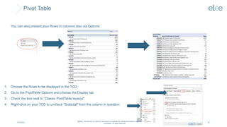
Excel offers real possibilities for data processing.
It is limited by the management of possible relationships between tables of data, as well as by the number of rows, in
this case 1,048,576.
Name Function
(ENG)
Name Function
(FR)
INDEX+MATCH INDEX+EQUIV
Returns a value or reference to a value from
an array or range of values. INDEX+MATCH
function does not know column limits on the
left (e.g. VLOOKUP)
(Array_column;MATCH(lookup_val
ue;lookup_array;0))
COUNTIFS NB.SI.ENS
Counts the number of cells within a range
that meet more than one criterion
(criteria_range1;criteria1;criteria_ra
nge2;criteria2…)
VLOOKUP RECHERCHEV
Returns a value from either a single-row or a
column range.
(lookup_value;lookup_array;col_in
dex_num;range_lookup[TRUE/FAL
SE])
SUMIFS SOMME.SI.ENS
Sums specified cells if they meet more than
one criterion.
(sum_range
;criteria_range1;criteria1;
criteria_range2;criteria2;…)

4/10/2024
32
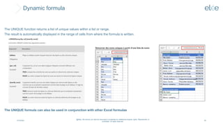
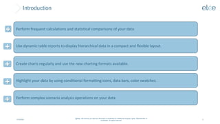
Excel allows you to process text-type data such as searching for one text in another, isolating the left or
right characters of a text, isolating words, counting characters or words in a text, etc. These types of
processing are ideal for organizing and structuring raw data received from another application.
Name Function
(ENG)
Name
Function (FR)
SEARCH CHERCHE
Renvoie la position du caractère dans une
chaîne correspondant au caractère recherché.
CHERCHE ne tient pas compte de la casse.
(find_text;text;within_text;[start_num]
)
VALUE CNUM
Convertit en nombre une chaîne de caractères
(texte) représentant un nombre.
(text)
RIGHT DROITE
Renvoie le(s) dernier(s) caractère(s) d’une
chaîne de texte, en fonction du nombre de
caractères spécifiés.
(text;num_chars)
LEFT GAUCHE
Renvoie le(s) premier(s) caractère(s) d’une
chaîne en fonction du nombre de caractères que
vous spécifiez.
(text;num_chars)
TEXTJOIN
JOINDRE.TEX
TE
Concaténation de la liste ou de la plage de texte
avec un délimiteur
TEXTJOIN(delimiter;ingnore_empty
(TRUE OR FALSE);text1…)
To concatenate multiple different values attached to a specific criterion, enter the following formula:
= TEXTJOIN(« delimiter »; TRUE;IF(logical_test;value_if_true; « »))
*we will see the logical function "IF" in more detail later

4/10/2024
33
Make calculations in PC
1. Calculate the total price of licenses used by product type;
2. Calculate the total price of all licenses used;
3. Calculate the average price per license;
4. Identify duplicates in the list of licenses;
5. Match the applicable discount for each product

4/10/2024
34
Formula
Formula “IF”
3

Formula – Formula “IF”
4/10/2024
35
If there were a list of the most used functions, the "IF" function would feature prominently!
It is a logical function that allows you to choose between two assumptions, based on a logical (or Boolean) expression.
A logical expression can take only two values: TRUE or FALSE.
SYNTAXE
= IF(logical_test;value1_if_true;value2_if_false)
Test: Logical expression.
A logical expression has at least one logical operator ( <;>;=;<>;...) and two operands.
Value1: A formula that can contain functions (including another SI function), calculations, a string, etc. This formula will
be used if Test is equal to TRUE.
Value2: A formula that can contain functions (including another SI function), calculations, a string, etc. This formula will
be used if Test is equal to FALSE.

4/10/2024
36
A few details on how to use the IF function
It is possible to develop a conditional formula based on a test involving numeric values, but also strings.
Dates are frequently used as test criteria. It is possible to use a conditional formula based on a date test.
In order to extend the possibilities of conditional formulas, it is possible to include functions (Mean, Sum, ...) in the test
criteria.
A conditional formula can also be used to avoid the display of error messages such as #DIV/0! Or #N/A, which often pollute
spreadsheets:
• OR we just have to test, for example, that the divisor of a formula (when it contains one!) is different from 0 (for #DIV/0),
• OR you can include your folmule "IF" in an "IFERROR" formula, specifying the value displayed in case of error:
=IFERROR(IF(logical_test;value1;value2); «value3 in case of error »)

4/10/2024
37
The conditional formulas used so far are "one-level", i.e. the result is a function of a single test, no matter how
complicated it may be. That said, some issues require the development of real decision trees, such as:
Si condition1 alors
Si condition2 alors
Si condition3 alors
Action1
Sinon
Action2
Sinon
Si condition4 alors
Action3
Sinon
Action4
Sinon
Si condition5 alors
Si condition6 alors
Action5
Sinon
Action6
Sinon
Si condition7 alors
Action7
Sinon
Action8
This is a nesting of IF functions, so that each of the "branches" of
the decision tree is set up. The arguments of the first IF function
are themselves IF functions, whose arguments are in turn IF
functions. Here we are dealing with a three-level nesting, which
materializes in the following way with the Excel syntax:
=IF(logical_test1;IF(logical_test2;IF(logical_test3;V
alue1_if_True; Value2_if_ False);
IF(logical_test4; Value3_if_True; Value4_if_
False));IF(logical_test5;IF(logical_test6;
Value5_if_True; Value6_if_ False);IF(logical_test7;
Value7_if_True; Value8_if_ False )))
IF
TRUE
IF
FALSE

4/10/2024
38
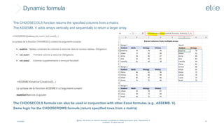
Si condition1 alors
Si condition2 alors
Si condition3 alors
Action1
Sinon
Action2
Sinon
Si condition4 alors
Action3
Sinon
Action4
Sinon
Si condition5 alors
Si condition6 alors
Action5
Sinon
Action6
Sinon
Si condition7 alors
Action7
Sinon
Action8
Up to 64 IF test levels can be nested. Suffice to say that some formulas may be illegible.
To make your complex formulas easier to read and write, you can insert line breaks as you type, using the
[Alt]+[Enter] key combination. The previous formula can thus be written as:
=IF(logical_test1;
IF(logical_test2;
IF(logical_test3;Value1_if_True;Value2_if_False);IF(logical_test4;Value3_if_True;Value4_if_False));
IF(logical_test5;
IF(logical_test6;Value5_if_True; Value6_if_ False);IF(logical_test7; Value7_if_True; Value8_if_ False )))
Sometimes it's easier to do complex analyses in PowerQuery* to simplify the writing of nested functions or other
tasks
*This topic is not covered in this training
IF
TRUE
IF
FALSE

4/10/2024
39
1. Using the simple "IF" formula, mark "YES" if a participant passed their test and "NO" if failed;
2. Using the nested "IF" formula, associate the score with each user based on their result;

4/10/2024
40
Formula
Formula “XLOOKUP”
3

Formula – Formula “XLOOKUP”
4/10/2024
41
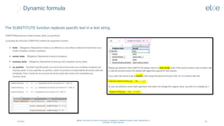
Benchmark you're
looking for
Data range where
to find the
reference value
The result you are
looking for in a data
range/column
Obligatory
Value to specify if
reference value is
not found
Match Type (Exact Match)
Search mode (e.g. starting with
the 1st or last element of the
table)
The XLOOKUP feature was introduced by Microsoft in 2019 and aims to replace VLOOKUP
(vertical search) and HLOOKUP (horizontal search)
VLOOKUP (37 years old in 2022!) allows you to search for a value in the first column of a data range, then return the corresponding value, on the same row, of the
desired column;
HLOOKUP (another old function) allows you to go the other way by looking for a value on the first row, before returning the data on the same column, to the
desired row;
XLOOKUP combines and fills in the gaps of the two specified functions (V&H). It works as follows:
=XLOOKUP(lookup_value; lookup_array; return_array; [if_no_found]; [match_mode]; [search_model])
Facultative

4/10/2024
42
The advantages of the XLOOKUP feature over the VLOOKUP.
By default, VLOOKUP doesn't look for an exact match; you need to specify the 4th parameter to FALSE to enable the exact match.
VLOOKUP works by specifying a column number (index); The function therefore does not support column deletions/insertions.
VLOOKUP looks exclusively to the right. With XLOOKUP, you can finally scan a board to the left!
VLOOKUP also does not allow you to return the last occurrence of a series of values. This is now possible with XLOOKUP.
XLOOKUP also allows you to search for the nearest upper approximate value, which VLOOKUP does not.
Finally, XLOOKUP avoids unnecessary calculations, since you can reduce your search field to an absolute minimum (noticeable
performance gains).

4/10/2024
43
1. Associate the ECC license names (from the mapping tab, column B) with the S4HANA license names (tab
1, column C) using the XLOOKUP formula;
2. Calculate the price of the ECC licenses used (quantities specified in tab 1 column D) by finding the unit
prices in tab 2 (mapping) column C via the XLOOKUP formula;

Pivot Table & Dynamic
formula
4

Pivot Table
4/10/2024
45
The Pivot Table (TCD) allows you to aggregate data by quickly composing a summary table
from a mass of data.
When sorting, filtering, and table tools are no longer enough to meet your needs, don't
hesitate create a pivot table. Before you start, however, it is essential to check the following
points:
The data range must have no empty rows or columns.
All columns must contain headings.
Delete all merged cells within the range of values

Pivot Table
4/10/2024
46
Click one of the cells in the data range
On the Insert tab, in the Tables group, click Pivot
Table.
In the Create PivotTable dialog box, verify that
Excel has selected the entire range of data.
In the Choose the location of your pivot table report.
Excel offers by default to use a new sheet, but it is
also possible to insert the TCD in the location of
your choice.

Pivot Table
4/10/2024
47
Excel creates a new sheet and places it to the left of the sheet that contains the data. Two new contextual tabs appear on
the ribbon, Analysis and Creation, as well as a pane on the right that contains the list of fields (the table headings) and four
areas with which you organize the data:
Consider renaming the sheet containing the pivot table.
Report Filter: Like all Excel filters, this area
filters the results according to a given
criterion.
Row Labels Accommodates fields
representing the row headings of the table.
Column Labels Accommodates fields
representing the column headings of the table.
Values Focuses calculations performed on
numeric or textual data.

Pivot Table
4/10/2024
48
The different manipulations related to the analysis aspect of TCD:
 Add data. You can also delete data that you don't want to analyze.
 Refresh to update the data in your workbook's pivot tables.
 Change the range of its data source.
 Delete a pivot table

Pivot Table
4/10/2024
49
The different manipulations related to the display aspect of TCDs:
 Change the layout of the data to make the table easier to read and analyze
 Change how subtotals, grand totals, and items are displayed.
 Change the table style as well as the TCD style options.

Pivot Table
4/10/2024
50
1. Choose the Rows to be displayed in the TCD;
2. Go to the PivotTable Options and choose the Display tab
3. Check the box next to "Classic PivotTable layaout"
4. Right-click on your TCD to uncheck "Subtotal" from the column in question
You can also present your Rows in columns also via Options:

Pivot Table
4/10/2024
51
1. Read the "Readme Quiz" tab first;
2. Create a new TCD from the table on the "Product Purchase Details" tab (new tab);
3. Bring up the view on the total quantity of licenses purchased but without Oracle Runtime and displaying
the product category;

Dynamic formula
4/10/2024
52
Microsoft is updating Excel 365 and making it very practical and simple to perform some calculations based on dynamic
formulas (rasters) that previously required a fairly advanced knowledge of the subject.
Today, with Excel 365, it is possible to process complex data quickly by extending these calculations automatically to
multiple columns and rows. Here are some examples
 Dynamically filter complex data;
 Find unique values;
 Sort data;
 Separate values (altrenative to "Text to Column")
 Select and display specific columns/rows of one or more table(s);
 Replace Characters in Text/Cell

Dynamic formula
4/10/2024
53
The purpose of the FILTER function is to filter complex data based on criteria of your choice.
The result is automatically displayed in the range of cells from where the formula is written.
The FILTER formula can also be nested and/or used in conjunction with other Excel formulas

Dynamic formula
4/10/2024
54
The UNIQUE function returns a list of unique values within a list or range.
The result is automatically displayed in the range of cells from where the formula is written.
The UNIQUE formula can also be used in conjunction with other Excel formulas

Dynamic formula
4/10/2024
55
The SORT function sorts the contents of a range or array.
The result is automatically displayed in an array in the same form as the provided array argument.
The SORT formula can also be used in conjunction with other Excel formulas

Dynamic formula
4/10/2024
56
The SPLIT function. TEXT works in the same way as the Column Text Wizard but as a formula.
Text is split into columns or rows (the inverse of the TEXTJOIN function)

Dynamic formula
4/10/2024
57
The CHOOSECOLS function returns the specified columns from a matrix.
The ASSEMB. V adds arrays vertically and sequentially to return a larger array.
The CHOOSECOLS formula can also be used in conjunction with other Excel formulas (e.g., ASSEMB. V).
Same logic for the CHOOSEROWS formula (return specified rows from a matrix)

Dynamic formula
4/10/2024
58
The SUBSTITUTE function replaces specific text in a text string.

Dynamic formula
4/10/2024
59
1. Read the "ReadMe" tab first;
2. Do the exercises in the following tabs:
• "2. Choose Columns"
• "3. Unique Values"
• "4. Smart Filter"

Data visualization
5

Data visualization
4/10/2024
61
It can be difficult to read and interpret data by going through multiple lines of information. You can use
conditional formatting to highlight certain data, allowing you to analyze data and identify patterns and
trends.
Highlight data by applying conditional formatting to cells
Data bar
Colour shades
Icon Sets
Data bars, color swatches, and icon sets are conditional
formatting that creates visual effects in your data. These
conditional formatting makes it easy to instantly compare
values across a range of cells.

Data visualization
4/10/2024
62
Data bars can help you identify the highest and lowest numbers,
such as licenses acquired and/or used by a customer. A longer bar
represents a larger value while a shorter bar represents a smaller
value.
Select the range of cells, table, or the entire sheet to which you
want to apply conditional formatting.
On the Home tab, in Format, click Conditional Formatting.
Point to Data Bars, and then click a gradient or solid fill.

Data visualization
4/10/2024
63
Color swatches help you understand the distribution and variation
of data, such as returns on investment over time. The cells are
stained with gradations of two or three colors corresponding to the
maximum, minimum, and average thresholds.
On the Home tab, in Format, click Conditional Formatting.
The top color represents the largest values, the center color, if it
exists, represents the average values, and the bottom color
represents the smallest values

Data visualization
4/10/2024
64
Use an icon set to present data in three to five categories based
on a threshold value. Each icon represents a range of values, and
each cell is assigned an icon representing its range. For example,
a set of three icons uses one icon to emphasize all values greater
than or equal to 67%, another icon for values less than 67% and
greater than 33%, and a final icon for values less than 33%.
Point to Icon Sets, and then click the icon set you want.
Icon sets can be combined with other conditional formatting.

Data visualization
4/10/2024
65
If, despite the diversity of choices, you don't find a predefined conditional formatting satisfactory, you
have the option to create your own rules. To do this:
Select the range to which you want the formatting to apply.
On the Home tab, click the Conditional Formatting button in the Style group.
Select New Rule.
In the New Formatting Rule dialog box, you can choose from several themes:
- Format all cells according to their value;
- Apply formatting only to cells that contain...;
- Apply formatting only to values that are among the first or last values;
- Apply formatting only to values above or below the average;
- Apply formatting only to unique values or duplicates;
- Use a formula to determine which cells will be formatted for.

Data visualization
4/10/2024
66
Use a formula to determine which cells the format will be applied to
These are rules for applying formatting to cells based on the result of a formula. If the result of the formula
is the logical value TRUE, the formatting will be applied. On the other hand, if the result of the formula is
the logical value FALSE, the formatting will not be applied.
To define a formatting rule:
Enter the formula in the box. It is possible to select a cell instead of entering a formula. The selected
cell must contain a formula that returns TRUE or FALSE.
Click the Format button to set the format to apply if the rule is satisfied.
Click the Preview button if you want to view the result on the spreadsheet.

Data visualization
4/10/2024
67
The Principle of Content Validation
Let's say you're designing a sheet in which users will enter information. Despite their best efforts, typing errors
will inevitably occur or the answers will not be homogeneous, making it difficult to process the data. In this
case, for example, validating the contents of cells allows you to define what is allowed and what is not allowed
in a cell.
To set up cell content validation:
Select the cell or range of cells you want to use.
On the Data tab, click the Data Validation button in the Data Tools group.
On the Options tab of the Data Validation dialog box, select the type of validation you want to apply, using the
Allow drop-down list.
Once you have chosen the type of validation, you need to define the corresponding validation criteria using the
Data drop-down list.
Click the Input Message tab. You can then enter a message that will appear when the cell is selected
(Example: with the separator ";" for a list of data).
Click the Error Alert tab. You can enter a message that will appear when the validation process does not
recognize value.

Data visualization
4/10/2024
68
Types of validation
Entitled Comments
Tout / Any value No restrictions on content. This is the default setting.
Nombre entier /
Whole number
Only whole numbers are allowed.
Décimal / Decimal Whole numbers and decimals are allowed.
Liste / List The allowed values are defined by an exhaustive list.
Semicolon-separated values can be specified in the
Source box, or reference to a range of cells
containing the allowed values can be specified in the
Source box.
Date Only dates are allowed.
Heure / Time Only hours are allowed.
Longueur du texte /
Text length
Restrictions on the length of text to be entered
Personnalisé /
Custom
Customize a text validation with a formula of
your choice

Data protection
6

Data protection
4/10/2024
70
Cells in a spreadsheet are protected to prevent other users from accidentally modifying them.
This is useful when the sheet contains complex formulas and essential data that require specific
protection.
Steps:
By default, protection is
enabled on calculation
sheets. However, this feature
is only enabled if the
protection of certain cells is
disabled:
1. Select the cells that will
be editable;
2. In the "Home" tab, click
on the triangle in the
"Font" group

Data protection
4/10/2024
71
Steps:
3. Select the "Protection"
tab and uncheck the
"Locked" box

Data protection
4/10/2024
72
Steps:
4. Select the "Review" tab,
then select the "Protect
Sheet" button;
5. Choose the protection
options (password, possible
actions to be performed on
the protected sheet)

Data protection
4/10/2024
73
Highlight the data as suggested in the PJ ("Quiz
Formatting – Test" tab)

Error messages
7

Error messages
4/10/2024
75
Errors in Excel formulas are manifested by the appearance of a small green triangle in the upper left corner of the
cell, as well as an error name preceded by the pound sign(#).
If you select a cell that contains an error, an exclamation mark in a yellow diamond appears to the left of the cell.
Clicking on this symbol brings up a drop-down list indicating the type of error and help to resolve it.
In some cases, one may decide to ignore the error.

SAM Training Session - How to use EXCEL ?

Recommended

Recommended

More Related Content

Similar to SAM Training Session - How to use EXCEL ?

Similar to SAM Training Session - How to use EXCEL ? (20)

Recently uploaded

Recently uploaded (20)

SAM Training Session - How to use EXCEL ?